Abstract

We describe a method to analyse inclined air showers produced by ultra high energy cosmic rays using an analytical description of the muon densities. We report the results obtained using data from inclined events ($60^{\circ}<\theta<80^{\circ}$) recorded by the Haverah Park shower detector for energies above $10^{19}~{}$eV. Using mass independent knowledge of the UHECR spectrum obtained from vertical air shower measurements and comparing the expected horizontal shower rate to the reported measurements we show that above $10^{19}$ eV less than $48\%$ of the primary cosmic rays can be photons at the $95\%$ confidence level and above $4\times 10^{19}$ eV less than $50\%$ of the cosmic rays can be photonic at the same confidence level. These limits place important constraints on some models of the origin of ultra high-energy cosmic rays.

1 Introduction

The question of the origin of cosmic rays (CRs) of the highest energies is currently a subject of much intense debate and discussion. The highest energy cosmic ray ($3\times 10^{20}$ eV) was detected by Fly’s Eye fluorescence detector [1] confirming the existence of cosmic rays with macroscopic energies above the Greisen, Zatsepin, and Kuz’min cut-off ($4\times 10^{19}$ eV) [2]. In addition the AGASA group have reported 8 events with energies above 100 EeV and other very energetic events with energies beyond the GZK cut-off have been described by the Volcano Ranch, Haverah Park and Yakutsk groups [3, 4, 5]. These ultra high-energy cosmic rays (UHECR) pose a serious challenge for conventional theories of CRs based on stochastic acceleration. The non-observation of the high energy cut-off expected because of the interactions with the Cosmic Microwave Background (CMB), indicates that their sources must be nearby thus posing serious restrictions as to their origin. There is currently a significant experimental effort underway, focussed around HiRes [6], the Pierre Auger Observatory [7] and EUSO [8], aimed at dramatically improving the statistics at the highest energies.

The old idea of attempting to detect high-energy neutrinos through studying very inclined air showers (HAS)[9] has been recently revived with the calculation of the acceptance of the Auger Observatories for the detection of high-energy neutrinos [10]. Ultra High Energy (UHE) neutrinos (above EeV) are almost inevitable in models that seek to explain the UHE cosmic rays. At large zenith angles, cosmic rays (whether they are protons, nuclei or photons) develop ordinary showers in the top layers of the atmosphere in a very similar fashion to the well-understood vertical showers. Their electromagnetic component is, however, almost completely absorbed by the greatly enhanced atmospheric slant depth (3000 g cm^-2 at 70^∘ from zenith) and thus prevented from reaching ground level. High energy neutrinos may induce HAS much deeper in the atmosphere close to an air shower array. By contrast, these showers at ground level resemble vertical air showers in their particle content and other features.

The main background to UHE neutrino induced HAS is expected to be due to the remaining muon component of the cosmic rays showers, after practically all of the electromagnetic component is absorbed. These $muonic~{}showers$ that penetrate the whole atmospheric depth to ground level are the object of this study. Although originally this project was conceived as a study of the background to neutrino-induced showers we have come to the conclusion that the interest in HAS induced by cosmic rays goes well beyond that expectation. The measurement of high zenith angle showers will enhance the aperture of the existing air shower arrays, and will increase the data on cosmic ray arrival directions to previously inaccessible directions in galactic coordinates [11]. Besides these obvious advantages, high zenith angle cosmic ray showers are unique because the shower front is dominated by relatively energetic muons that travel long distances, opening up the possibility of probing interactions in a region of phase space quite inaccessible in vertical air showers.

Cosmic ray induced HAS are different from vertical showers mainly because they consist largely of muons which are produced far from ground level. The particle density profiles for HAS induced by protons or heavy nuclei display complex muon patterns at the ground which result from the long path lengths traveled by the muons in the presence of the Earth’s magnetic field [12, 13]. These patterns are difficult to analyse [14] and invalidate the conventional approach used for interpretation of low zenith angle showers ($<60^{\circ}$), which is usually based on the approximate circular symmetry of the density profiles. The analysis of HAS produced by cosmic rays requires a radically different approach such as the one presented in this work.

We apply our approach to data recorded by the Haverah Park experiment. The Haverah Park array, being made of 1.2 m deep water Čerenkov tanks [15], is the detector array so far constructed which is best suited on geometrical considerations for the analysis of very large inclined showers. Moreover it can be considered as a prototype of the Auger Observatories, which will employ water Čerenkov tanks of identical depth. The quantitative aspects of our results are very specific to the water Čerenkov technique as we have previously taken into account in great detail the interaction of the shower particles in the water detectors [16].

In this paper we give a much more detailed account of a report already published [17]. The present work is organized as follows: In section 2 we discuss the main features of inclined showers, the muon distributions, the different sources of electrons and photons and the shower front curvature. In section 3 we give a brief description of the Haverah Park array, its detectors and their response to the passage of different particles from the shower front. In section 4 we develop an algorithm reconstruct the arrival directions and energies of inclined air showers detected with Haverah Park. In section 5 we describe a procedure to generate artificial events based on shower generation and measurements of the cosmic ray spectrum. In section 6 we compare the high zenith angle data to the artificial event distributions obtained under different assumptions about the nature of the primary particles that constitute the cosmic ray energy spectrum above $10^{19}$ eV. We extract bounds on photons above $10^{19}$ eV. Finally in section 7 we discuss our results and review their implications. In a subsequent paper we will describe the use of this technique to yield the proton/iron ratio as a function of energy above 1 EeV.

2 Inclined air showers

As the zenith angle varies from the vertical, $\theta=0^{\circ}$, to the horizontal, $\theta=90^{\circ}$, direction, the slant matter depth rises from $\sim 1000$ to $\sim 36000$ g cm^-2 and for angles above $60^{\circ}$ the cosmic ray showers at ground level are observed well past the shower maximum. In inclined showers of zenith angles exceeding $70^{\circ}$ the electromagnetic component arising from the hadron shower through $\pi^{0}$ decay can be neglected at ground level. For zenith angles between $60^{\circ}$ and $70^{\circ}$ the relative signal of this component in a 1.2 m deep water Čerenkov detector is small except for distances within a few hundred meters from shower axis. While the electromagnetic component of air showers is exponentially attenuated with depth, the muons that are too energetic to decay, have few catastrophic interactions and only suffer ionization losses, scattering and geomagnetic deflection. They constitute the dominant component of the shower front for inclined showers. The muon patterns at ground level have been studied in [18]. There is a residual electromagnetic component in the shower front which is produced by the muons themselves, mostly through muon decay. Other muon interactions contribute either little to the electromagnetic component or only within a narrow region about shower axis.

2.1 The muon component

The distribution of the muon component at ground level becomes complex at large zenith angles because of magnetic field effects. The spatial distribution of muons can no longer be characterized by a simple function of one parameter (distance to the shower axis, $r$) because of the asymmetry generated mostly by the geomagnetic effects. In [18] an analytic model to account for the average muon number densities at ground level in presence of a magnetic field for proton showers at high zenith angles is presented and described in detail. We outline its main features because the work presented here relies heavily upon it.

The approach consists of studying the muon distributions in the absence of magnetic field effects so that they have cylindrical symmetry to an excellent approximation. The distributions are described by functions of one variable ($r$), the lateral distribution functions, in a plane perpendicular to the shower axis, the transverse plane. A very strong anticorrelation between the average muon energy and distance of the muon from the shower axis has been described [18].

Magnetic deviations of the muons are subsequently applied to the circularly symmetric distributions, making use of the aforementioned anticorrelation and assuming the muons are produced in a fixed region of the atmosphere. The magnetic distortions induced in the muon distributions are described by considering the projection of the Earth’s magnetic field onto the transverse plane. As the zenith angle increases the patterns obtained in the transverse plane gradually change from elliptical distributions to two lobed figures reflecting an increased distance traveled by the muons which results in enhanced distortions. The double lobe patterns correspond to positive and negative muons totally separated by the magnetic field which acts as a spectrometer for the muons in the shower. Moreover as the azimuth changes, both the magnitude of the magnetic field projection onto the transverse plane and its relative orientation with respect to the ground, change, further increasing the diversity of the resulting patterns projected onto the ground.

The description of the average muon density patterns thus requires three inputs:

$\bullet$ The lateral distribution function (LDF).

$\bullet$ The average muon energy as a function of radius (${\cal E}(r)$).

$\bullet$ The mean distance to the muon production point ($l_{0}(\theta)$).

All these values must first be evaluated in the absence of magnetic effects. The model also requires knowledge of the muon energy distribution at a fixed distance to the shower axis. A log-normal distribution of width 0.4 has been found to be sufficiently accurate for all practical purposes.

The validity of the analytical description has been evaluated by comparing full shower simulations for different arrival directions with those obtained by this procedure. A comparison of muon densities in this model to those obtained by simulation is shown in Fig. 1. The simulations of the density distributions both with and without the magnetic field have been made with the AIRES [19] code. Tests for proton showers using the SIBYLL [20] hadronic interaction generator at a fixed energy of $10^{19}$ eV, and four different zeniths are described in [18].

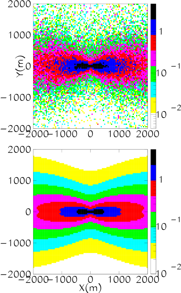
Figure 1: Contour plots of the muon density patterns in the transverse plane for $10^{19}$ eV proton showers with an incident zenith angle of $\theta=80^{\circ}$ and azimuth angle $\phi=0^{\circ}$ as obtained in the simulation (upper panel) and with the analytic approach described (lower panel).

This approach is independent of model details and can be applied to other hadronic generators, mass compositions, and energies by changing the corresponding inputs. It allows the comparison of muon density patterns at ground level through these simple inputs. A significant advantage is that, provided the lateral distribution function is parameterized by a continuous function, the muon density patterns obtained in the transverse plane are smooth functions in contrast to distributions obtained with any Monte Carlo simulation. This key point allows us to reconstruct the energy of individual events, as we describe below.

We have also found [16] that to a good approximation the inputs to our model are energy independent for a given primary, so the muon number density distributions for any primary energy can be obtained simply by normalizing the total number of muons of a fixed energy shower. These results apply to showers both with and without the magnetic field. The energy dependence of the normalization factor can be obtained by monitoring the total muon number in the showers ($N_{\mu}$). The values of $N_{\mu}$ from simulations are plotted in Fig. 2 for four different zenith angles. The energy dependence of the normalization can be taken into account accurately by a simple relation of the following form:

$$N_{\mu}=N_{0}~{}\left[{E\over 10^{19}~{}{\rm eV}}\right]^{\beta},$$ (1)

where $N_{0}$ (the number of muons at $10^{19}$ eV) and $\beta$ are constant parameters for a given hadronic interaction model and mass composition. For different zenith angles the energy scaling index, $\beta$, is the same and only the normalization $N_{0}$ changes.

Figure 2: The relationship of total muon number to primary energy for protons of four zenith angles using the QGSJET model [31].

Furthermore the muon distributions at ground level are hardly different in shape for iron and proton. This is illustrated in Figs. 3 and 4 where muon densities patterns and densities along given lines parallel to the $x$ and $y$ directions in the transverse plane axes are compared for iron and proton primaries. To a good approximation the differences can be accounted for by differences in the total number of muons. For a given model and primary composition the energy dependence of very inclined showers can be parameterized with only two parameters. In Table 1 the results for these two parameters for proton and iron in two interaction models are shown.

Model	A	$\beta$	$N_{\mu}$ ($10^{19}$ eV)
SIBYLL	1	0.880	1.6 107
	56	0.873	2.2 107
QGSJET	1	0.926	2.1 107
	56	0.909	2.8 107

Table 1: Relationship between muon number and primary energy for different models and primary masses (see Eq. (1)), for a zenith angle of 60^∘.

Figure 3: Muon density patterns in the transverse plane for a $10^{19}~{}$eV proton shower incident with $80^{\circ}$ zenith angle, as well as for an iron shower normalized to the same number of muons for comparison.

Figure 4: Top left panel: Muon number density in the transverse plane as a function of the $x$ coordinate for a fixed value of $y$ as obtained with the model for a proton (full line) and iron (dashed line) shower of $10^{19}~{}$eV arriving with 80^∘ zenith angle. The $y$-axis is chosen parallel to the magnetic North. Densities are calculated in 40 m x 40 m bins and the $x$ axis bins shown are centered at $y=0$. Bottom left panel: ratio of for proton and iron densities along the $x$ axis. Top right panel: Muon number density taking $y$ bins for a fixed value of $x$= 1000 m. Bottom right panel: density ratio along the $y$ coordinate.

It is well known that fluctuations in shower development can enhance the trigger rate for air showers produced by lower energy primaries because of the steep cosmic ray spectrum. The fluctuations to larger numbers of particles allow some of the more numerous low energy showers to trigger the detector. We have also studied muon number fluctuations at ground level and how they relate to shower development (mean muon production height) and average muon energy. We have found that the mean muon energy correlates strongly with production height but that most of the number density fluctuations can be accounted for by fluctuations in muon number. Fluctuations in the total number of muons are mainly due to fluctuations in the depth of maximum, which are related to fluctuations in the first interaction depth, as well as to fluctuations in the neutral to charged pion ratios in the first interactions. In Fig. 5 the distribution of the muon number for a set of 100 showers with the same primary energy and mass composition is plotted. Although the distribution is slightly asymmetric with a tail towards low $N_{\mu}$ number, in this work we have assumed a gaussian distribution with a width of $\sigma_{N_{\mu}}=0.2<N_{\mu}>$. In Fig. 5 we compare the mean muon density as a function of $r$ to that of the extreme cases of muon rich and muon poor showers obtained in the simulation. No significant changes in the shape of the muon LDF need to be considered for distances beyond about 100 m.

Figure 5: Left panels: Distribution of the total number of muons for 100 individual proton showers of energy $10^{19}~{}$ eV and zenith angle $60^{\circ}$ (top graphs), $75^{\circ}$ (bottom graphs), simulated with AIRES code and QGSJET hadronic generator. Right panels: Muon lateral distribution for the extreme showers with largest and lowest number of muons compared to the mean.

Fluctuations in the number of muons in photon-induced showers are rather different from those in hadron-induced showers. If the first interaction of the incident photon happens to be hadronic (probability R$\sim$ 0.01 at $10^{19}$ eV) then the shower is indistinguishable from a hadronic shower. For the distribution of the total number of muons in a photon shower we can therefore expect a long tail of showers with large number of muons, as can be seen in Fig. 6.

Figure 6: Distribution of number of muons for individual photon showers at $10^{19}~{}$ eV simulated with AIRES code and QGSJET hadronic generator. This plot was obtained combining different zenith angles normalizing the number of muons of each individual shower to the mean value at a given zenith angle.

2.2 The electromagnetic component of very inclined showers

As will be described in the next section a detector that uses water Čerenkov tanks is more efficient for detecting muons than electrons and photons because muons typically go through the whole tank and thus give larger signals in the tanks than the typically lower energy electrons and photons. The electromagnetic component of inclined shower induced by a proton or a nucleus has been studied with the help of both analytical calculations and Monte Carlo simulations using the AIRES code [19]. We can distinguish three components according to their origin:

Figure 7: The average longitudinal development of the muon (continuous line) and electron (dashed lines) components for 100 proton showers of energy $10^{19}$ eV and different zenith angles. At depths exceeding 3000 g cm^-2, or equivalently for zenith angles greater than 70^∘, the electromagnetic component is mainly due to muon decay.

$\bullet$ The component fed by muon decay: The longitudinal developments of the electron and muon components are shown in Fig. 7 for $10^{19}~{}$eV proton showers arriving with four different zenith angles. In these simulations the effects of muon bremsstrahlung, pair production and nuclear interactions are not included. The most striking feature of these figures is that after reaching shower maximum there is a residual component that follows closely the muon depth distribution. This effect is mostly due to electrons from muon decay. The relative number of electromagnetic particles (electrons and photons) with respect to the muons is seen to be practically independent of depth and only mildly increasing with zenith angle.

As electrons and photons develop from multiple electromagnetic subshowers their energy distribution is essentially the same as that of a typical air shower. The ratio fluctuates because of the discreteness of the energy deposition. The lateral distribution follows that of the muons rather closely, as shown in Fig. 8 unlike the LDF for electrons in near vertical air showers.

$\bullet$ The component fed by $\pi^{0}$ decay: Fig. 7 clearly shows an early electromagnetic part mostly induced by the $\pi^{0}$’s from the hadronic interactions which decay into photons that cascade down the atmosphere. This component becomes exponentially suppressed after shower maximum and is quite unimportant for inclined showers. Indeed even at $60^{\circ}$ the electromagnetic component of a $10^{19}$ eV proton shower which can be directly associated to $\pi^{0}$ decay is already low and confined within a relatively small region of about 200 m around shower axis. For $\theta>70^{\circ}$ we do not have a significant contribution to the electromagnetic component from $\pi^{0}$ decay.

$\bullet$ The component fed by muon interactions (bremsstrahlung, pair production and muon nuclear interactions): The muons in very inclined air showers have greater energies and traverse more matter than in the vertical case so these processes need to be considered. We have estimated the global bremsstrahlung contribution by considering the muon energy spectrum of a single shower, folding it analytically with the bremsstrahlung cross-section and the Greisen parameterization, see [21]. For an $80^{\circ}$ zenith and $10^{19}~{}$eV proton shower the total number of electrons and positrons ($N_{e}$) obtained is about $2.5~{}10^{4}$. These are mostly due to the muons in the energy range between 30 GeV and 500 GeV. This component arises also from electromagnetic sub-showers and its energy distribution should also reflect that of electromagnetic cascades. If we multiply, conservatively, the total number of electrons by a factor three to account for the two other muon interactions, it is still a factor of $\sim$50 below the total number of muons in the shower, and negligible compared to the electromagnetic contribution from muon decay. This component has recently been incorporated into a new version of AIRES and analysed fully with simulation in [22]. These results show that the electromagnetic component dominates over the muons only for distance to shower axis below $\sim 100$ m in agreement with our calculations.

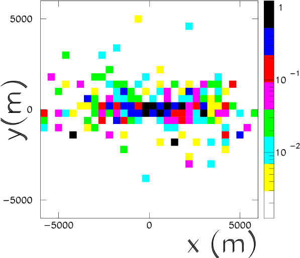
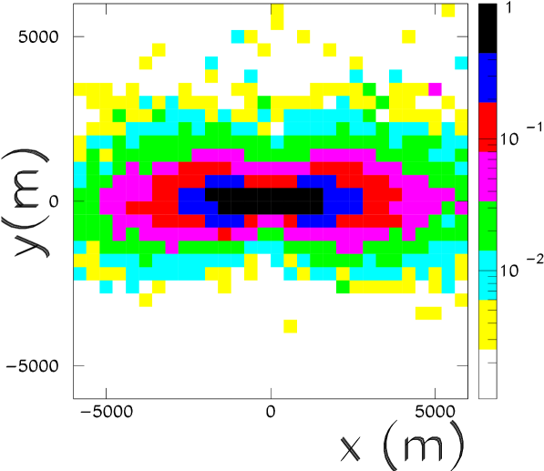
Figure 8: Left: Density pattern of the muons in the transverse plane for a $10^{19}$ eV proton induced shower with a zenith of $80^{\circ}$, and including geomagnetic effects. Right: Electron density pattern for the same shower.

To evaluate the relative importance of each of these contributions to the shower front relative to the signal induced by the muons in inclined showers, we need to weight the different type of particles at ground with the signal produced by them in a given experiment. In section 3 it will be shown that the quantitative effects of the electromagnetic component for water Čerenkov tanks such as those used in the Haverah Park array are unimportant except for distances very close to the shower axis.

2.3 Shower front curvature

Very inclined air showers detected at ground level are mostly dominated by muons which travel long distances without large attenuations, as discussed in the previous section. We expect the curvature and the time spread of the muon front to be smaller than in vertical showers. We have studied the arrival time of the muons through simulations performed with AIRES code. We have simulated 100 proton induced showers at $10^{19}$ eV for three different zeniths ($60^{\circ}$, $70^{\circ}$, and $80^{\circ}$). The output from the simulation gives the arrival time of the muons at ground level, but we prefer to study the shower front (thickness and shape) in the transverse plane. We have projected the muons onto the transverse plane, correcting the arrival times at the ground with the different muon paths to reach this plane. After this correction we get the time distributions of the muons for different bins in distance to the shower axis.

Figure 9: Distribution of distances traveled by the muons from their production site to the ground for three different zeniths. The ratio of $\sigma/d$ for the three histograms are 0.4, 0.27 and 0.20 respectively. At 87^∘ (not shown) the ratio is 0.13.

The distance traveled by the muons characterizes the most important properties of the shower front in inclined showers and is the basis of the analytical model discussed in section 2.1. It also characterizes the curvature of the shower front. Assuming the muons are produced at a fixed point one would expect a spherical shower front which turns out to be a fairly good approximation. The distributions of distances traveled by the muons from the production site to the ground are plotted in Fig. 9 for three different zeniths, as obtained from simulations. The distributions are relatively narrow compared to the mean value $<$$d$$>$, so that for a given zenith angle it is a reasonable approximation to consider all the muons as coming from a fixed point. As the production point is not very sensitive to the nature of the primary particle the curvature of the shower front can be also expected to be relatively independent of composition.

Typically the times recorded in a ground array experiment, which are eventually used for the arrival direction fit, are the relative times of the onset of the signal at the different detectors. One can visualize the muon arrival time distribution as the delay associated with the different muon paths from production to a particular position in the shower front. We take from the time distribution the arrival time of the first muon. This implies that there is another factor that can distort an experimental reconstruction of the shower front related with the statistical sampling. For a given number of muons $n$ arriving at a particular detector, we are effectively sampling the corresponding time distribution $n$ times and then choosing the earliest time. For a large number of muons, this time will tend to the geometrical delay of the highest energy muon, but for a small number of muons the earliest muon will be distributed about a mean value with a width which decreases with $n$. As a result there is an additional curvature that is entirely a statistical effect as was pointed out many years ago [23].

In Fig. 10 we have plotted the arrival time of the first muon in the sample for four different zeniths and assuming a different number of muons hit the detector. We have superimposed a spherical front with radius of curvature equal to $<d>$. The accuracy of this simple approximation seems good enough except for very high zeniths. As the muon number density drops with the distance from the shower axis, the sampling will affect the measured arrival time of the first muons. The curvature effectively grows with the distance to the shower axis. This can be accounted for as an extra contribution to the error of the measured time. In an experimental situation the necessity of spherical corrections will be determined by the experimental errors in relation to the arrival time delays. We will apply curvature corrections in the event reconstruction of inclined showers in section 4. A spherical front assumption seems justified except for showers close to the horizontal when a flat front can be assumed because the curvature is very small.

Figure 10: Arrival times of the first muon at different distances from the shower axis for a $60^{\circ}$, $70^{\circ}$, $80^{\circ}$, and $87^{\circ}$ proton induced shower, after sampling the time distributions for different number of muons. Dots correspond to a sampling with 1 muon, open squares to 10 muons, and stars to 100 muons. The continuous line plotted corresponds to a spherical shape with the radius of curvature equal to the mean distance traveled by the muons to ground ($<d>$).

3 The Haverah Park array

The Haverah Park (HP) extensive air shower array was situated at an altitude of 220 m above sea level (mean atmospheric depth=1016 g cm^-2) at 53^∘ 58^′ N, 1^∘ 38^′ W. The particle detectors of the shower array were water Čerenkov counters. The detectors consisted of a number of units of varying area built from water Čerenkov tank modules. The modules were of two types. The majority were galvanized iron tanks 2.29 m² in area, filled to a depth of 1.2 m with water and viewed by one photomultiplier with 100 cm² photocathode. A minority of detectors were 1 m${}^{2}\times$ 1.2 m deep-water Čerenkov detectors constructed from expanded plastic foam. Detector areas larger than 2.29 m² were achieved by grouping together a number of the larger modules in huts. Fig. 11A shows the layout of the Haverah Park array.

The trigger rate of an air-shower array at large zenith angles is extremely sensitive to the geometry of the array. Factors such as the shape and relative altitude of detectors become very important for such showers. The relative altitudes and orientations of the four A-site detectors, the triggering detectors, are shown in Fig. 11B. A gradient across the array is apparent and this has a significant effect on the observed azimuthal distribution. Fig. 11C shows the positions of individual tanks within the thermostated huts that housed the detectors. The signals from 15 of the 16 tanks, each of area 2.29 m², were summed to provide the signal used in the trigger. One tank in each hut was used to provide a low gain signal. See [15] for a more detailed description of the array.

The signal released in a water Čerenkov detector is proportional to the energy lost in the tank by ionization. As most of the energy of a vertical air shower at ground level is carried by the electrons and photons, this technique is very effective at measuring the energy flow in the shower disc. Water-Čerenkov densities were expressed and recorded in terms of the mean signal from a vertical muon (1 vertical equivalent muon or VEM). It has been shown that this signal is equivalent to approximately 14 photoelectrons (pe) for HP tanks [24]. The formation of a trigger was conditional on: (i) A density of $>0.3$  VEM m^-2 in the central detector (A1) and (ii) at least 2 of the 3 remaining A-site detectors recording a signal of $>0.3$ VEM m^-2. The rates of the triggering detectors were monitored daily. Over the life of the experiment, after correction for atmospheric pressure effects, the rates of the detectors were stable to better than 5$\%$. Approximately 8000 events with zeniths exceeding $60^{\circ}$ were recorded during an on time of $3.6~{}10^{8}$ s between 1974 and 1987.

Figure 11: The Haverah Park Array. A) The 2 km array. B) The relative heights and orientations of the A-site detector huts. C) The arrangement of water tanks within an A-site detector hut.

3.1 Detector response

The calculation of the water-Čerenkov signal from inclined showers is complex. The simulation of the propagation of vertical and inclined electrons, gammas, and muons of different energies through Haverah Park tanks has been performed using a specifically designed routine WTANK [25] which uses GEANT [26]. The mean signal of electrons, gammas and muons have been convolved with the particle distributions obtained in the shower simulations to calculate the measured signal at ground by the water tanks for different zenith angles. Details of this calculation can be found in [16].

The signal produced by Čerenkov light from the muons in the Haverah Park tanks is proportional to the track which typically goes through the whole tank. For a given muon density the signal is also proportional the tank area and as a result the mean signal is proportional to the tank volume and independent of the arrival direction of the shower relative to the tank. At large zeniths the smaller cross sectional area presented by the tank means that fewer muons than for vertical showers make up the same average signal by having longer tracks. Therefore Poisson fluctuations in the total number of muons going through a tank become more important for large zenith angles.

The signal produced by very inclined muons is enhanced by two processes. For very inclined showers it is possible for Čerenkov photons to fall directly onto the PMT without reflection from the tank walls (we refer to such photons as “direct light”). Also the mean muon energy rises with zenith so that the probability of interaction in the tank is increased because both the cross sections and the average amount of water traversed increase. The production of secondary electrons via pair production, bremsstrahlung, nuclear interactions (collectively referred to as PBN interactions), and electron knock-on ($\delta$-rays) is therefore enhanced. For example the correction due to $\delta$-ray production increases from 2 pe at typical vertical muon energies of 1 GeV to around 3 pe for $>10$ GeV. These contributions have been parameterized as a function of zenith and azimuth for each of the different geometries of detectors that were used in the HP array.

On the other hand the electromagnetic particles in inclined showers usually get completely absorbed in the tanks and the output signal is just proportional to the input particle energy. Thus their contribution to the total signal at larger zenith angles is suppressed compared to muons because of the reduction of the projected area of the detectors. In Fig. 12 we show the ratio of electromagnetic to muon signal as simulated in a Čerenkov tank of 1.2 m depth (as used in Haverah Park and being implemented for the Auger Observatory) as a function of distance to the shower axis for a vertical shower compared to two showers at large zenith angle. The shower particles have been fed through the tank simulation as if they were coming from the vertical direction to eliminate geometric tank effects. The results illustrate the behaviour of the electromagnetic to muon signal ratio because of the ratio of electromagnetic particles to muons varying with zenith angle and distance to shower axis $r$. It is well know that the muon lateral distribution is flatter than that for the electromagnetic component and thus the ratio decreases below 1 for $r$ greater than $\sim 800~{}$m for vertical showers. The graph illustrates that already for zenith angles of $\sim 60^{\circ}$ this ratio is around the $25\%$ level for $r>200~{}$m and that for zeniths above this value this ratio at $1.5$ km is still about a factor 3 smaller than for vertical showers. The rise of the ratio in Fig. 12 at small distances to the core can be attributed to the pion showering process combined with $\pi^{0}$ decay.

Figure 12: The ratio of the electromagnetic to muon contributions to water-Čerenkov signal as a function of distance from the shower axis. The non uniformity of the curves is due to statistical fluctuations.

We have averaged the water-Čerenkov signal induced by muons and electromagnetic particles for $r<2~{}$km. In Fig. 13 we plot the average electromagnetic signal induced per muon, measured in VEM. The behaviour of this curve has as minimum at $\theta\simeq 67^{\circ}$. For zenith angles smaller than this there is still a contribution from the electromagnetic component from $\pi^{0}$ decay so the ratio is increasing rapidly as we move towards lower zenith angles. For zenith angles above this minimum the electromagnetic signal is dominated by muon decay which again increases at very large zenith angles. As the electromagnetic signal tends to be completely absorbed in the tank, the shape of the tanks is not important for this figure. We have parameterised the percentage contribution of the signal due to muon decay relative to the muons as a linear function on $\sec\theta$ independently for proton, iron and gamma primaries, see Fig. 13. These relative values are useful for event simulation on the basis of the muon density maps.

Also shown is the ratio of average signals induced by electromagnetic particles to that of the muons. This last curve shows how the relative contribution to the measured signals of electromagnetic particles decreases with zenith angle, in spite of the increase of the absolute electromagnetic signal per muon. This is because the muons from very inclined showers give enhanced signals in the tanks because of geometry.

Figure 13: Ratio of the total signal from muons and electromagnetic particles arriving within 2 km from the shower core as a function zenith angle. The dots corresponds to the case in which the muons are fictitiously assumed to enter in the tank parallel to the vertical direction and the squares corresponds to the real signal given by a muon at the corresponding zenith angle (including direct light, knock-on electrons,..). The plot was done with 100 proton showers at $10^{19}~{}$ eV simulated with AIRES and QGSJET hadronic generator for each zenith angle. The curve shown corresponds to the fit described in the text.

After subtracting the flat component due to muon decay we have plotted in Fig. 14 the remaining electromagnetic contribution to the signal in a specific HP tank configuration (the triggering tanks) for $60^{\circ}$, $62^{\circ}$, $64^{\circ}$ and $66^{\circ}$ as a function of the distance to the shower axis. This is the contribution from $\pi^{0}$ decay with large errors because of the subtraction procedure. We have also plotted the muonic contribution including geometric effects and enhancements due to direct light and muon interactions. As the zenith angle increases the electromagnetic contribution is suppressed. It can be seen that the electromagnetic contribution due to $\pi^{0}$ decay is only relevant at small distances($<200~{}m$) to the shower axis. This contribution to the electromagnetic component has been parameterized as a function of zenith for proton, iron and photon primaries fitting the curves in Fig. 14 to a Haverah Park type [27] lateral distribution function.

Figure 14: The mean electromagnetic signal due to the showering process and $\pi^{0}$ decay in a HP tank (circles) compared to the muon signal (stars) as a function of distance to the shower axis for four different zenith angles. The plot was done with 100 proton showers at $10^{19}~{}$ eV simulated with AIRES and QGSJET hadronic generator. The large errors in the mean electromagnetic signals are statistical.

4 Event reconstruction

The distortion of the circular symmetry in very inclined air showers prevents the use a single parameter to measure the shower energy. This is in contrast to near-vertical showers for which the measurement of the density at 600 m $\rho(600)$ has been shown to be fairly independent of composition for the Haverah Park array [28]. Because of energy scaling of the muon number that controls the recorded signal at large angles, the natural way to obtain the energy of single events is to fit the energy and core position simultaneously to the expected density maps appropriate to the corresponding arrival direction. We describe our approach below.

4.1 Direction reconstruction

The Haverah Park arrival directions were determined originally using only the 4 central triggering detectors . We have reanalyzed the arrival directions of showers having original values of $\theta$ $>56^{\circ}$, taking into account all detectors which have timing information. This reanalysis produces smaller arrival direction uncertainties due to the larger baselines involved.

The curvature of the shower front has been investigated in section 2 using the AIRES code for inclined showers. The measurement error of the times recorded by HP array is $\sim 40$ ns, so from Fig. 10 it is apparent that the shower front is consistent with the approximation of a spherical front centred at the mean muon distance to production site (e.g. at 60^∘ the radius of curvature is 16 km). Beyond $\sim 80^{\circ}$ curvature effects are rather small and it is quite sufficient to assume a plane front [29]. When the detected muon number is small there is a systematic effect on the curvature correction and large fluctuations due to limited sampling of the shower front. Therefore, we used only the timing information from detectors with $>15$ equivalent muons detected.

The direction fits of the data were originally performed using the maximum likelihood algorithm described in [30], which is only suitable to fit to a plane front. The uncertainty used in making the plane fit was:

$$\Delta t({\rm ns})=\Delta t_{m}+{20{\rm ns}\over\sqrt{N_{\mu}}}\,,$$ (2)

where $\Delta t_{m}$ is the measurement error ($\sim~{}40~{}$ ns), and the second term is added to account for sampling errors.

To fit the direction taking into account the curvature effects we first fitted the recorded times to a plane front. Then each measured time was corrected for curvature effects and the fit was repeated. If the resulting zenith angle differed by more than $0.1^{\circ}$ from the previous one, times were again corrected and the fit repeated. The iteration was terminated when convergence had been achieved (i.e. $\delta\theta<0.1^{\circ}$). Because of the dependence of the curvature fit on the position of the shower core, the iterative process must also involve fits to the particle density to obtain the core position. The implementation of this complex iterative procedure will be described in a subsection 4.4. The uncertainty expression used in the curvature fit is:

$$\Delta t({\rm ns})=\sqrt{\Delta t_{m}^{2}+\Delta t_{c}^{2}+\Delta t_{s}^{2}}\,,$$ (3)

where $\Delta t_{c}$ is the error induced in the corrected times by the uncertainty in the core position, $\Delta t_{m}$ is the measurement error, and $\Delta t_{s}$ is the sampling error (see subsection 2.3 ).

4.2 Parameterizations for the muon densities

We have obtained the inputs needed in our analytical description of muon densities [18] from specific AIRES simulations with the QGSJET [31] hadronic interaction generator. For three possible compositions of proton, iron and gamma primaries, one hundred showers were generated for each zenith angle in the range $60^{\circ}$ - $89^{\circ}$ (in $1^{\circ}$ steps) in the absence of a magnetic field, at a fixed energy of $10^{19}$ eV. Using the procedure described in [18], we have prepared a compact library of muon density patterns at a fixed energy for different zenith angles and different compositions. Magnetic deviations are accounted for in the muon distributions projecting the Earth’s magnetic field onto the transverse plane and using the algorithm described in [18] which rotates the pattern depending on the azimuthal direction. Different energies were obtained through energy scaling as indicated in subsection 2.1.

The electromagnetic component is separated into two parts:

$\bullet$ The component fed by muon decay: In the previous section we showed that the contribution to the signal in the tanks due to electromagnetic particles produced by muon decay was present at all core distances and that it made a contribution to the signal that depends slightly on zenith angle and is of $\sim 3$ photoelectrons per arriving muon. The spatial distributions of this electromagnetic contribution follows the muon density pattern, so it is relatively simple to include it using the density maps described above.

$\bullet$ The component fed by $\pi^{0}$ decay: The tail of the electromagnetic part of the shower contributes mildly to the particle density at ground level at zenith angles below $70^{\circ}$ and core distances less than 500 m. This contribution has been modeled using AIRES with QGSJET (see previous section) and is radially symmetric in the transverse plane. The tail of the electromagnetic part of the shower contributes 20 % of the total water-Čerenkov signal at 400 m from the core for a $60^{\circ}$ shower. As is clear from Fig. 14, the contribution drops both for larger distances and for higher zenith angles. This electromagnetic component was calculated at an energy of $10^{19}~{}$ eV: the values for different energies were obtained by scaling with energy ($\rho_{em}\propto E_{0}$).

4.3 Detector signal conversion

We will later on compare the signal at the detectors to predictions based on simulation of showers. For each detector we will compare the recorded number of muons $N_{\mu}^{r}$ to the number of muons predicted from a given density map $N_{\mu}^{p}$, which is simply obtained multiplying the muon number density by the transverse area for each detector. The actual values of $N_{\mu}^{p}$ used are corrected to account for the electromagnetic contribution due to the tail of the showering processes. We now describe the process of converting the actual recorded signal to $N_{\mu}^{r}$ which is not straight forward because of several corrections that need to be considered.

The detector signals were recorded in units of vertical equivalent muons. Using the GEANT based package, WTANK [25], we have found that this unit corresponds to an average number of 14 photoelectrons, in agreement with experimental estimates [24]. For inclined showers additional effects, such as direct light on the photomultiplier tubes, delta rays, pair production and bremsstrahlung by muons inside the tank, increase this number. For a given zenith angle, we have calculated the mean number of photoelectrons per muon ($pe_{\mu}$) taking into account all the processes mentioned before except for pair production and bremsstrahlung. Pair production and bremsstrahlung do not alter the expected rate as a function of zenith angle by more than a $1\%$, so we have not included this effect to save computing time.

To calculate the value of $pe_{\mu}$ we use:

$$pe_{\mu}=(pe_{vem}+pe_{\delta})\frac{A_{v}}{A_{h}(\theta,\phi)}+pe_{em}(\theta)+pe_{dl}(\theta)\,,$$ (4)

where $pe_{dl}$ is the contribution from the direct light, $pe_{em}$ is the contribution of the electromagnetic part from muon decay which is $\sim 3$ photoelectrons per arriving muon. The first term is the contribution proportional to the muon track, including the Čerenkov light from both the muon track ($pe_{vem}$) and from the $\delta$ rays ($pe_{\delta}$), which have to be corrected by the ratio of the vertical to the inclined average tracklength. This correction can be also expressed in terms of the ratio of the cross sectional areas presented by the tanks for vertical and inclined muons ($A_{v}/A_{h}$) as explained in subsection 3.1.

The different sizes of detectors present in Haverah Park array are described in Table 2 with their corresponding areas, density thresholds and saturation densities. These differences have forced us to simulate with WTANK the different detector geometries for different zenith angles to obtain the corresponding values of $pe_{\mu}$.

Type	Vert. area ($m^{2}$)	Thresh. (VEM $m^{-2}$)	Sat.(VEM $m^{-2}$)
Trigger detectors	37.	0.	45.
2 km array	14.	0.	45.
150 m array	9.	0.	60.
Infill array	1.	7.	-
J,K,L detectors	2.25	7.	-

Table 2: Characteristics of the different kind of detectors in the Haverah Park array

The recorded signals at each detector are first converted into the corresponding number of photoelectrons by multiplying the recorded density (m^-2) by the vertical area and the number of photoelectrons per vertical muon (14 pe). The number of muons going through each tank, $N_{\mu}^{r}$, is then obtained dividing this number of photoelectrons by the number expected per muon at the corresponding arrival direction $pe_{\mu}$, given in Eq. (4). For detectors that saturate or have thresholds, the corresponding number of muons $N_{\mu}^{sat}$ and $N_{\mu}^{th}$ are calculated for a given arrival direction in an analogous fashion using the saturation and threshold signals of Table 2.

4.4 The fitting algorithm

The observed densities were fitted against predictions using the maximum likelihood method. The quantity to maximize in this method is:

$$\ln~{}P(x_{c},y_{c},E_{0})=\ln(P_{1}~{}P_{2}~{}....~{}P_{n})=\sum_{i=1}^{n}~{}\ln~{}P_{i}\,,$$ (5)

where $n$ is the number of detectors used in the fit and $P_{i}$ is the probability that the $i^{th}$ detector records $N_{\mu}^{r}$ muons if the predicted number of muons is $N_{\mu}^{p}$ (as obtained from the muon density maps). The primary energy $E_{0}$ and the core coordinates ($x_{c},y_{c}$) are the free parameters in the fits. In order to calculate the probabilities needed in Eq. 5 we assume a Poisson distribution with mean $N_{\mu}^{p}$ given by:

$$P_{i}=\frac{\left(N_{\mu}^{p}\right)^{r}e^{-N_{\mu}^{p}}}{r!}\,,$$ (6)

where $r$ is the closest integer to $N_{\mu}^{r}$. When large numbers of muons ($N_{\mu}^{r}>8$) are involved we approximate the Poisson distribution with a gaussian distribution with mean $N_{\mu}^{p}$ and width $\sigma$ obtained adding three different errors in quadrature:

$$\sigma=\sqrt{\sigma_{p}^{2}+\sigma_{m}^{2}+\sigma_{g}^{2}}\,,$$ (7)

where $\sigma_{p}=\sqrt{N_{\mu}^{p}}$ is the Poisson error of the muon number, $\sigma_{m}$ is the measurement error ($7\%$ of the recorded signal), and $\sigma_{g}$ is the error induced by geometrical considerations: dependence of the detector area with azimuth and azimuthal variations of the direct light. The main contribution to $\sigma$ comes from $\sigma_{p}$. If the detector is saturated the corresponding probability is calculated integrating the gaussian distribution from $N_{\mu}^{sat}$ to $\infty$. If the detector density is under the threshold we evaluate the Poisson probability of getting $N_{\mu}^{th}$ or fewer muons.

A three-dimensional grid search was made to maximize Eq. 5 finding the most likely impact point and shower energy. The energy was varied in the range $10^{17}<E_{0}^{p}<10^{21}$ eV in steps of $0.1$ in $\log_{10}(E_{p}/\mbox{eV})$. The impact point was varied over a grid of 12 km $\times$ 6 km in 40 m steps in the perpendicular plane, the grid asymmetry being necessary to accommodate the ellipticity of inclined showers.

Since angle reconstruction depends on the core position for curvature corrections a complex algorithm was required to avoid spurious dependences between core location and direction determination. The steps of the algorithm to find the final parameters of an event are the following:

$\bullet$ 1- Find $\theta$, and $\phi$ by fitting a plane front to the times registered by the triggering detectors.

$\bullet$ 2- With the reconstructed direction, find the core position and primary energy through a three dimensional grid search, maximizing the likelihood function.

$\bullet$ 3- Find a new value for $\theta$, and $\phi$ fitting a plane front to the times registered by the detectors within 1 km of the core (found in the previous step) in the shower plane. If there are less than 7 detectors with time information we complete the number with the next nearest detectors, which may lie $>1$ km from the shower axis.

$\bullet$ 4- With the reconstructed direction, find a new core position and primary energy.

$\bullet$ 5- Repeat step 3 and 4 once to avoid any bias induced by the first determination of the shower core (which used a direction fitted with a small number of times from detectors that could be far away from the shower core).

$\bullet$ 6- Find $\theta$ and $\phi$ taking into account the curvature in the front. This yields the final reconstructed direction. We also calculate $\Delta\theta$. The zenith angle does not usually change more than $1^{\circ}$ compared with the value obtained in the previous step.

$\bullet$ 7- With the reconstructed direction, find again the core position and primary energy ($x_{c},y_{c},E_{0}$). This will be the final reconstructed parameters of the event.

$\bullet$ 8- Find core position and primary energy for changes to the value of $\theta$ by $\theta+\Delta\theta$ and $\theta-\Delta\theta$. This step is particularly important for controlling and understanding the systematic uncertainty of the primary energy due to the zenith angle uncertainty.

Errors in the energy and core determination were determined from the likelihood function as described in [32]. In addition to this error, an error in energy arises due to the uncertainty in the zenith angle. The error from the zenith angle determination and the error from the fit are added in quadrature to give the total error shown in Table 3. The typical error in the position of the core is $100$ m and in $\log_{10}E_{0}$ it is $0.1$, corresponding to $26\%$.

4.5 Results of the data fit

Over 8000 events were fitted with muon density maps generated for proton primaries and the QGSJET hadronic generator, following the procedure explained in the previous subsection.

To guarantee the quality of events the following cuts were made to the reconstructed events: (i) the distance from the central triggering detector to the core position in the shower plane is required to be below $r_{max}=2$ km, (ii) the $\chi^{2}$ probability for the energy and direction fits must be $>$ 1 %, (iii) the downward error in the energy determination is required to be less than a factor of 2. The chosen value of $r_{max}$ guarantees that the core position is always surrounded by detectors in the HP array. After making the cuts described above we found 52 events with $E_{0}>10^{19}$ eV, ten events with energies above $4\times 10^{19}$ eV and one with energy above $10^{20}$ eV. For zenith angles greater than $80^{\circ}$ no showers pass cut (iii).

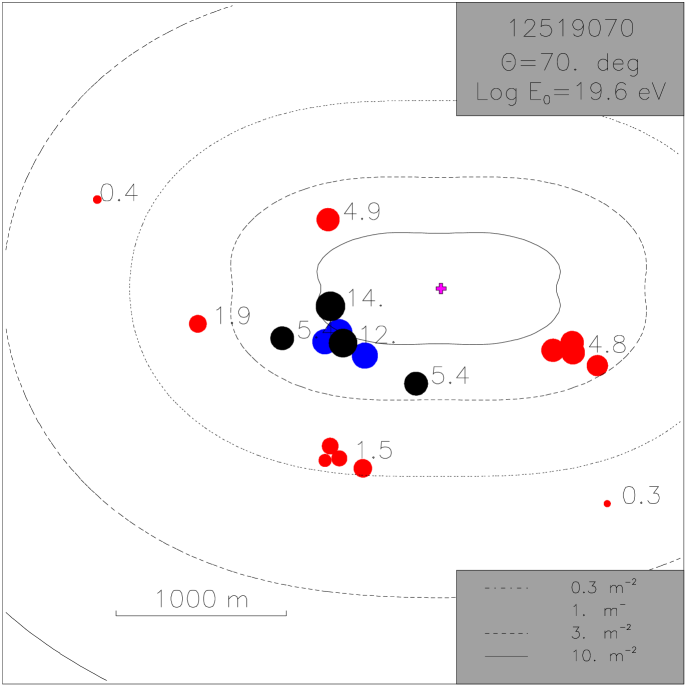
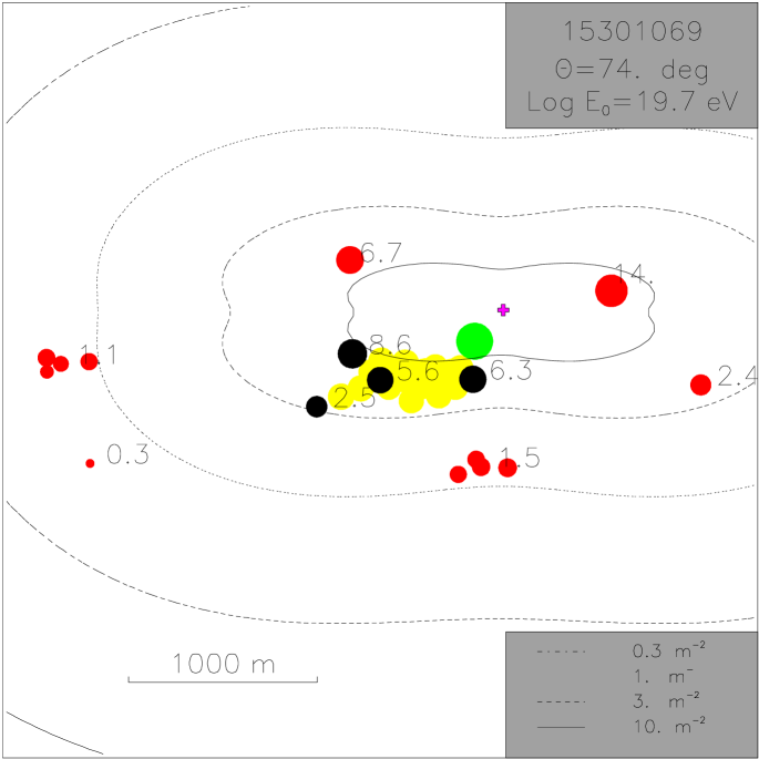
Figure 15: Density maps of two events in the plane perpendicular to the shower axis. Recorded muon densities are shown as circles with radius proportional to the logarithm of the density. The detector areas are indicated by shading; the area increases from light grey to black as 1, 2.3, 9, 13, 34 m². The position of the best-fit core is indicated by a cross. Selected densities are also marked. The $y$-axis is aligned with the component of the magnetic field perpendicular to the shower axis.

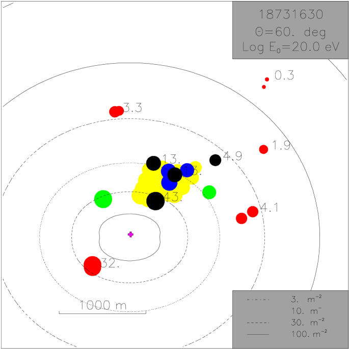
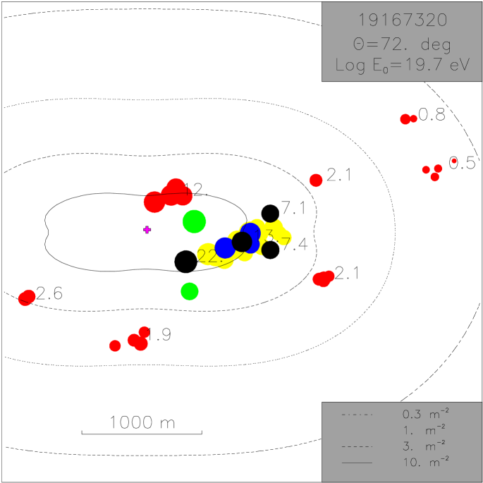
Figure 16: Same as Fig. 15

In Figs. 15 to 16 the density maps for four reconstructed events are shown in detail. These maps are plotted in the plane perpendicular to the shower direction together with the contours of densities that best fit the data. In each figure the array is rotated in the shower plane such that the $y$-axis is aligned with the component of the magnetic field perpendicular to the shower axis. In Fig. 15 and on the right panel of Fig 16 the asymmetry in the density pattern due to the geomagnetic field is apparent. For all these events the core is surrounded by recorded densities and is well determined. In table 3 details are given of the 10 events with $E_{p}>4\times 10^{19}$ eV.

MR	Zenith (∘)		RA (∘)	Dec. (∘)	$\log_{10}(E_{p}/\mbox{eV})$			$\chi^{2}/\nu$
18731630	60	$\pm$2.3	318.3	3.0	20.04	-0.03	+0.03	40.0/42
14050050	65	$\pm$1.2	86.7	31.7	19.89	-0.08	+0.10	11.0/13
18565932	68	$\pm$1.3	46.4	6.0	19.88	-0.22	+0.34	15.5/15
25174538	65	$\pm$1.2	252.7	60.2	19.85	-0.22	+0.20	5.0/5
14182627	70	$\pm$1.3	121.2	8.0	19.76	-0.05	+0.05	5.0/10
15301069	74	$\pm$1.2	50.0	49.4	19.76	-0.06	+0.05	27.1/32
19167320	72	$\pm$1.3	152.5	25.9	19.75	-0.06	+0.04	36.5/33
12753623	74	$\pm$2.1	304.9	17.1	19.67	-0.07	+0.10	11.4/11
24503624	69	$\pm$2.1	16.9	53.0	19.63	-0.22	+0.33	11.0/9
12519070	70	$\pm$1.3	47.7	8.8	19.62	-0.08	+0.06	15.2/14

Table 3: Zenith angle, arrival direction coordinates and shower energy (assuming proton primary) of selected showers with energy $>4\times 10^{19}$ eV. MR is the event record number. The reported $\chi^{2}$ values and the degrees of freedom ($\nu$) refer to the density fits.

This work improves and extends the results presented in [17] and is compatible with it. There are however slight differences which are due to the improvements, namely:

1. Improved muon density parameterizations, now in $1^{\circ}$ steps.

2. Inclusion of densities below threshold in the fitting algorithm.

3. Better treatment of the electromagnetic part of the shower from muon decay.

4. Inclusion of events with original zenith angle $56^{\circ}<\theta<60^{\circ}$.

The inclusion of three additional events in table 3 compared with what was obtained in [17], and the changes in the energies of some events should be noted. It must be stressed that the new energy always lies within the error quoted in [17], and the three new events were not included in the original list because they failed to pass the cut on the downwards error.

The photoelectron distributions in a water detector show long tails due to the processes mentioned in section 3.1. We therefore expect an excess of upward fluctuations over downward fluctuations from the average detector signal. For each event we calculate the probability that each of the detectors involved has a signal which deviates by more than $>$2.5$~{}\sigma$ from the average using the simulated photoelectron distributions. We reject signals having (upward or downward) deviations greater than 2.5 $\sigma$, recalculating the best-fit core after any rejection. Of 226 densities in the events described below and listed in table 3 we have rejected 12 upward deviations (the expected number was 17) and a single downward deviation. We consider this to be a strong vindication of our understanding of the signal in the tanks and of our modeling procedures.

5 Generation of artificial events

Besides the fitting of the individual events it is extremely important to compare the data obtained with expectations. We have simulated “artificial” events assuming a given energy spectrum for the cosmic rays, taken from other experiments and assuming different primary compositions. In order to compare the simulated results to those obtained from the data, we must also calculate the reconstruction efficiency which is sensitive to the cuts made. Throughout we use the QGSJET as the hadronic generator of the simulations.

We have generated showers in the range of energies $10^{18}$ eV to $10^{21}$ eV in bins of 0.05 in $\log_{10}E_{0}$. For each of these energy bins we have adjusted the number of artificial events generated to approximately obtain $300$ showers that trigger the array. The procedure for generating each artificial event is the following:

1. We randomly select an arrival direction assuming isotropy according to a $\sin\theta$ distribution for zenith angle and a uniform distribution for azimuth ($\phi$).

2. Each shower is directed on to the array with a random impact point position in the transverse plane up to 2.5 km away from the centre of the array.

3. Each time a shower is directed at the array, the total muon number($N_{\mu}$) is fluctuated to take into account shower fluctuations. For proton and iron primaries we used a gaussian distribution of spread 0.2$~{}N_{\mu}$, and for photon primaries we used the distribution in Fig. 6.

4. The density in the ground plane at the location of each of the detectors is read from the library of muon density maps.

5. The corresponding signal and arrival time in each of the detectors is generated (see next subsection).

6. The trigger condition of the Haverah Park array is tested.

7. If an event is deemed to trigger the array then the density and time information is recorded in the same format as the real data.

8. Each artificial event is assigned a weight ($w_{o}$) which is $N_{exp}/N$, where $N$ is the total number of events generated in a particular energy bin, fulfilling, or not, the triggering condition and $N_{exp}$ is the total number of CR expected from the assumed flux for the same energy bin integrated over the zenith angle range considered ($59^{\circ}-89^{\circ}$).

The artificial events, recorded in the same format as real data, are analysed with the same algorithm assuming a proton composition for the maps and with QGSJET as the hadronic generator, and applying the same cuts. The resulting spectrum is obtained by adding the weights of the individual artificial events at the corresponding reconstructed energies.

5.1 Implementation of the signal in the detectors

The signal in each detector is artificially generated as follows:

1. The projected area of the detector in the shower plane is calculated.

2. Given the local muon density and the projected area, the number of incident muons is sampled from a Poisson distribution.

3. The track length of each muon through the detector is sampled from a distribution obtained analytically from the detector geometry (see Fig. 11C).

4. The contribution of indirect Čerenkov light from the incident muons and from $\delta$-ray electrons is calculated from the sampled track lengths (12 pe for each 1.2 m of track, with an additional 3 pe/1.2 m to account for the signal from $\delta$-rays).

5. The signal from direct light on the PMTs is related to the detector geometry in a more complex way and is implemented using WTANK to simulate the passage of muons through the whole detector for a range of zenith and azimuth angles.

6. The electromagnetic component of the shower due to muon decay is approximated by the addition of a number of photoelectrons per muon ($n$) which depends smoothly on zenith angle.

7. The electromagnetic component of the shower from $\pi^{0}$ decay is calculated using the parameterizations discussed in section 3.

8. The signal generated in this way is fluctuated according to measurement errors.

The arrival time of the first muon is generated assuming a spherical shower front with radius equal to the mean distance to the production site of the muons at each particular zenith angle. The time is then fluctuated according to measurement and sampling errors.

5.2 Comparison of data and artificial event distributions

We assume a recent parameterization of the energy spectrum given in [33] noting that the agreement between the fluorescence estimates of the spectrum and those made by other methods implies that we have an approximately mass independent knowledge of the spectrum measured in the near-vertical direction. The flux above 10¹⁹ eV is assumed to be known to within 20$\%$ uncertainty. We will compare to the results obtained using an alternative energy spectrum given in [34]. Both fluxes are compared in Fig. 17.

Figure 17: Parametrizations of the cosmic ray flux between 10¹⁸ and 10²⁰ eV used in this work due to Nagano-Watson [33] (dashed line) and to Szabelski et al. [34] (full line) compared to AGASA data [35].

In Fig. 18, 19, 20, 21 we show different output parameters of the event reconstruction for the artificial events assuming a proton composition and the spectrum given in [33], compared to data. All the events used in these figures pass the cuts described in the previous section, in particular for energies above $10^{19}$ eV, $r_{max}=2~{}$km. The agreement obtained is encouraging and suggests that the simulation accurately mimics the data.

In Fig. 22 we show the energy resolution for different energy ranges. A finite energy resolution has the effect of increasing the measured rate by misinterpreting more abundant lower energy events as having a higher energy. However no corrections need be made in this approach because the same effect is present both in data and simulations.

Figure 18: $\chi^{2}$ distributions from the energy and direction reconstruction of data (stars) and artificial events (histogram), assuming proton composition and the parameterizations of the spectrum given in [33].

Figure 19: Downward and upward error distribution in the reconstructed energy from the density fits to the data (stars) and to the artificial events (histogram).

Figure 20: Zenith angle distribution for data (stars) and artificial events (histogram). No normalization has been made. Statistical error bars are also shown.

Figure 21: Left Panel: distribution of errors in zenith angle from the fit for the data (stars) and artificial events (histogram). Right panel: distribution of the difference between the real and the reconstructed zenith angle.

Figure 22: Energy resolution integrated for all zeniths in different energy bins. A flat energy distribution is assumed for each graph.

6 Limits on composition

After all the quality cuts are implemented as discussed in section 4 we calculate the event rate as a function of the primary energy integrating over all zenith and azimuth angles. We will concentrate here on the events with reconstructed proton energy above $10^{19}~{}$eV, which provide the most stringent conclusions about UHECR composition.

In Fig. 23 we show both the integral and differential energy spectra obtained from the artificial events under three different assumptions for the primary composition (protons, iron and photons) compared to the data using the cosmic ray parameterization given in [33]. We also show the spectra obtained using the cosmic ray flux spectrum from [34], see Fig. 24. All curves are for the QGSJET hadronic interaction model. The agreement between the curves generated for protons with the two spectra is remarkable. The normalization of the curves has not been manually adjusted. The expected rate increases if iron is assumed and decreases if photons are assumed. This just a matter of counting muons, heavier nuclei have more muons while photons are known to have much fewer muons. For the same reason shifts in the curves can be expected if different hadronic interaction models are used according to the number of muons they predict.

Figure 23: Integral (left panel) and differential (right panel) number of inclined events as a function of energy for the Haverah Park data set (*stars) compared to the predictions for iron (dotted line), protons (continuous) and photon primaries (dashed). The parameterization of the spectrum given in [33] is assumed.

Figure 24: Integral (left) and differential (right) number of inclined events as a function of energy for the Haverah Park data set compared to the predictions for iron, protons and photon primaries. The parameterization of the spectrum given in [34] is assumed.

The remarkable point about this graph is that the expected rate for photons is about an order of magnitude below the proton prediction. Assuming that cosmic rays have a proton/photon mixture at ultra high energies it is easy to obtain a bound from this graph. We can get bounds on photon abundance at a given confidence level comparing the measured number of events above a given threshold and its error to the expected numbers in the case of proton and photon compositions, taking into account the uncertainty in the prediction from the normalization error in the parameterization of the cosmic ray spectrum. Assuming the prediction obtained with the flux in [33] we obtain that less than $48\%$ of the observed events above $10^{19}~{}$eV can be photons with a $95\%$ confidence level. Above $4\times 10^{19}$ eV less than $50\%$ can be photons at the same confidence level. If we assume the spectrum of [34] instead the bound for photon increases (decreases) to $25\%$ ($70\%$) at energies above $10^{19}~{}$eV ($4\times 10^{19}~{}$eV).

The results for the photon bound depend on the hadronic model we choose but in a way that is conservative. If we were to chose a model that produces fewer muons that QGSJET we would predict a composition heavier than protons. If we chose a model that produces more muons, we would require a lighter composition and more photon flux would be allowed. From the KASCADE project [36] it is evident that all models tested except for sibyll produce muon rates above that found in the data. So models that produce more muons are disfavoured.

Our photon bound is also conservative because we have not taken into account the interactions of the high energy photons in the magnetic field of the Earth [37]. This has the effect of converting a single energetic photon into a few lower energy photons. As the total number of muons in a shower initiated by a single photon scales approximately with $E^{1.2}$, the number of muons in a shower initiated by a single photon exceeds the total number of muons if the photon energy is split into multiple photon showers of lower energy.

The implementation of photohadronic interactions in the AIRES code [19] and CORSIKA code [38] (using the parameterization of [39]) give predictions of the total number of muons that are equal to within 10% at $10^{19}$ eV. Unless the photoproduction cross section has a dramatic increase at high energies, the photon bound is robust because the photoproduction cross section is small relative to hadronic interactions.

7 Discussion

Conventional acceleration mechanisms, so called ”bottom up” scenarios, predict an extragalactic origin with mainly proton composition as although nuclei of higher charge are more easily accelerated they are fragile to photonuclear processes in the strong photon fields to be expected in likely source regions [40]. ”Top down” models explain the highest energy cosmic rays arising from the decay of some sufficiently massive “X-particles”. These models predict particles such as nucleons, photons and even possibly neutrinos as the high energy cosmic rays, but not nuclei. In some models [41, 42, 43] these X-particles are postulated as long-living metastable super-heavy relic particles (MSRP) clustering in our galactic halo. For these MSRP models a photon dominated primary composition at $10^{19}$ eV is expected. Other top down models [44] associate X-particles with processes involving systems of cosmic topological defects which are uniformly distributed in the universe, and predict a photon dominated composition only above $\sim 10^{20}$ eV.

On general grounds dominance of photons over protons is expected for these models due to the QCD fragmentation functions of quarks and gluons from X-particle decays into mesons and baryons. The ratio of photons to protons for MSRP models is typically 10 [41] at 10¹⁹ eV from QCD fragmentation. However some models predict a ratio closer to 2 [42]. The difference depends on distance to the sources because the photons attenuate in shorter distances than the protons in the cosmic microwave background and thus can become suppressed relative to the protons if the sources are distant. Clearly, our bound on the photon flux puts severe constraints on some ”top down” models. This is illustrated in Fig. 25 where this ratio is plotted for three such models and compared to our bound.

Figure 25: Photon to proton abundance ratio as a function of the energy for three different models for the origin of high energy cosmic rays by Berezinsky et al. (BKV) [41], Birkel et al. (BS) [42], and Rubin [43]), and the $95\%$ CL bounds presented in this work.

Observations above $10^{19}$ eV are otherwise consistent with both top down and bottom up interpretations [1, 45]. There is however some partial evidence against the photon hypothesis. Shower development of the highest energy event [1], is inconsistent with a photon initiated shower [46] while AGASA measurements of the muon lateral distribution of the highest energy events are compatible with a proton origin [48]. Our result has been recently confirmed by comparing muon and electron densities in vertical air showers detected by the AGASA array [47].

Here we have described a new method to analyse inclined showers. The method opens up a new way to measure cosmic ray showers. These showers are complementary to vertical showers because they are mostly due to muons that are produced far away from the detection point. The method can be applied to array detectors that use water Čerenkov tanks such as the Auger observatories now in construction.

The power of analysing inclined showers is illustrated with the analysis of the Haverah Park data. This analysis has allowed us to set the first limit to the photon content of the highest energy cosmic rays. We conclude that observations of inclined showers provide a powerful tool to discriminate between photon and proton dominated compositions.

Acknowledgements: We thank Gonzalo Parente for suggestions after reading the manuscript. This work was partly supported by a joint grant from the British Council and the Spanish Ministry of Education (HB1997-0175), by Xunta de Galicia (PGIDT00PXI20615PR), by CICYT (AEN99-0589-C02-02) and by PPARC(GR/L40892).

References

- [1] D.J. Bird et al., Phys. Rev. Lett. 71 (1993) 3401, and Astrophys. J. 441 (1995) 144.
- [2] K. Greisen; Phys. Rev. Lett., 16 (1966), 748. G.T. Zatsepin and V.A. Kuz’min, JETP Lett., 4 (1966), 78. Pisma Zh. Eksp. Teor. Fiz. 4 (1996) 114.
- [3] J. Linsley, Phys. Rev. Lett. 10 (1963) 146; Proc. 8th International Cosmic Ray Conference 4 (1963) 295.
- [4] B.N. Afanasiev et al, Proc. Tokyo Workshop on Techniques for the Study of Extremely High Energy Cosmic Rays (ed. M. Nagano, Inst. for Cosmic Ray Research, University of Tokyo) (1993) p 35.
- [5] M. A. Lawrence, R. J. O. Reid, and A. A. Watson, J. Phys. G Nucl. Part. Phys. 17 (1991) 733, and references therein.
- [6] T. Abu-Zayyad et al., Nucl. Instrum. Meth. A450 (2000) 253; (http://www.comic-ray.org).
- [7] The Pierre Auger Project Design Report, by Auger Collaboration, FERMILAB-PUB-96-024, Jan 1996; ( http://www.auger.org)
- [8] O. Catalano and L. Scarsi, in Proc. of the Int. Workshop on Observing Ultra High Energy Cosmic Rays from Space and Earth, (2000) Metepec, Puebla, Mexico, to be published by AIP.
- [9] V.S. Berezinsky and A. Yu. Smirnov, Astrophys. Space Science 32 (1975) 461.
- [10] J. Capelle, J.W. Cronin, G. Parente, and E. Zas, Astropart. Phys. 8 (1998) 321.
- [11] M. Ave, R.A. Vázquez, E. Zas, J.A. Hinton, and A.A Watson, Proc. of XXVI Int. Cosmic Ray Conf., Utah, (1999) vol.2 p. 365.
- [12] A.M. Hillas et al., Proc. of the XI Int. Cosmic Ray Conf., Budapest (1969), Acta Physica Academiae Scietiarum Hungaricae 29, Suppl. 3, p. 533-538, (1970);
- [13] D. Andrews et al., Proc. of the XI Int. Cosmic Ray Conf., Budapest (1969), Acta Physica Academiae Scietiarum Hungaricae 29, Suppl. 3, p. 337-342, (1970).
- [14] E.E. Antonov et al., Pis’ma Zh. Éksp. Teor. Fiz. 68 (1998) 177 (JETP Letts. 68 (1998) 185).
- [15] R.M. Tennent, Proc. Phys. Soc. 92 (1967) 622.
- [16] M. Ave, J.A. Hinton, R.A. Vázquez, A.A. Watson, and E. Zas, Astropart. Phys. 14 (2000) 107.
- [17] M. Ave, J.A. Hinton, R.A. Vázquez, A.A. Watson, and E. Zas, Phys. Rev. Lett. 85 (2000) 2244.
- [18] M. Ave, R.A. Vázquez, and E. Zas, Astropart. Phys. 14 (2000) 91.
- [19] S.J. Sciutto, AIRES: A System for Air Shower Simulation, Proc. of the XXVI Int. Cosmic Ray Conf. Salt Lake City (1999), vol. 1, p. 411-414; preprint archive astro-ph/9911331.
- [20] R.T. Fletcher, T.K. Gaisser, P. Lipari, and T. Stanev, Phys. Rev. D50 (1994) 5710; J. Engel, T.K. Gaisser, P. Lipari, and T. Stanev, Phys. Rev. D46 (1992) 5013.
- [21] E. Zas, F. Halzen, and R.A. Vázquez, Astropart. Phys. 1 (1993) 297.
- [22] A.N. Cillis and S.J. Sciutto, Phys. Rev. D64 (2001) 013010.
- [23] A.J. Baxter, PhD Thesis (1967), University of Leeds.
- [24] A. Evans, PhD Thesis (1971), University of Leeds.
- [25] J.R.T. de Mello Neto, WTANK: A GEANT Surface Array Simulation Program, GAP note 1998-020.
- [26] R. Brun et al., GEANT, Detector Description and Simulation Tool, CERN, Program Library CERN (1993).
- [27] R.N. Coy et al., Astropart. Phys. 6 (1996) 263.
- [28] A.M. Hillas et al., Proc. 12th Int. Cosmic Ray Conf., Hobart 3 (1971) 1001.
- [29] X. Bertou, P. Billoir, and T. Pradier, GAP Note 58 (1997); (http://www.auger.org/admin/).
- [30] A.J. Baxter, PhD thesis, University of Leeds, p 24, (1967).
- [31] N.N. Kalmykov and S.S. Ostapchenko, Yad. Fiz. 56, (1993) 105; Phys. At. Nucl. 56(3), (1993) 346; N.N. Kalmykov, S.S. Ostapchenko, and A.I. Pavlov, Bull. Russ. Acad. Sci. (Physics) 58, (1994) 1966.
- [32] M. Lampton, B. Margon, and S. Bowyer, Astrophys. J. 208, (1976) 177.
- [33] M. Nagano and A.A. Watson, Rev. Mod. Phys. 72, No. 3 (2000) 689.
- [34] J. Szabelski, T. Wibig, and A.W. Wolfendale, Astropart. Phys. (to be published).
- [35] M. Takeda et al., Astrophys. J. 522, (1999) 225.
- [36] KASCADE collaboration. Proc. of XXVI Int. Cosmic Ray Conf., Utah, (1999) vol.1 p. 135.
- [37] B. McBreen and C.J. Lambert, Phys. Rev. D24 (1981) 2536; X. Bertou, P. Billior, and S. Dagoret-Campagne, Astropart. Phys. (to be published).
- [38] D. Heck, J. Knapp, J.N. Capdevielle, G. Shatz, and T. Thouw, Forschungzentrum Karlsruhe Report FZKA 6019 (1998).
- [39] T. Stanev, T.K. Gaisser, and F. Halzen, Phys. Rev. D32, (1985) 1244.
- [40] A. M. Hillas, Ann. Rev. Astron. Astrophys. 22 (1984) 425.
- [41] V.S. Berezinsky, M. Kachelriess, and A. Vilenkin, Phys. Rev. Lett. 79, (1997) 4302.
- [42] M. Birkel and S. Sarkar, Astropart. Phys. 9, 297 (1998).
- [43] N.A. Rubin, MPhil thesis, University of Cambridge (1999).
- [44] P. Bhattacharjee, C.T. Hill, and D.N. Schramm, Phys. Rev. Lett. 69 (1992) 567; R.J. Protheroe and T. Stanev, Phys. Rev. Lett. 77, (1996) 3708.
- [45] N. Hayashida et al., Phys. Rev. Lett. 73 (1994) 3491; S. Yoshida et al., Astropart. Phys. 3, (1995) 105; M. Takeda et al., Phys. Rev. Lett. 81, (1998) 1163.
- [46] F. Halzen, R.A. Vázquez, T. Stanev, and H. P. Vankov, Astropart. Phys. 3 (1995) 151.
- [47] K. Shinozaki et al., Proc. of XXVII Int. Cosmic Ray Conf., Hamburg, (2001) vol.1 p. 346.
- [48] M. Nagano, D. Heck, K.Shinozaki, N. Inoue, and J. Knapp, Astropart. Phys. (to be published), astro-ph/9912222.