Modelling surface magnetic field evolution on AB Doradûs due to diffusion and surface differential rotation

Abstract

From Zeeman Doppler images of the young, rapidly-rotating K0 dwarf AB Doradûs, we have created a potential approximation to the observed radial magnetic field and have evolved it over 30 days due to the observed surface differential rotation, meridional flow and various diffusion rates. Assuming that the dark polar cap seen in Doppler images of this star is caused by the presence of a unipolar field, we have shown that the observed differential rotation will shear this field to produce the observed high-latitude band of unidirectional azimuthal field. By cross-correlating the evolved fields each day with the initial field we have followed the decay with time of the cross-correlation function. Over 30 days it decays by only 10%. This contrasts with the results of ? who show that on this timescale the spot distribution of He699 is uncorrelated. We propose that this is due to the effects of flux emergence changing the spot distributions.

1 Introduction

AB Doradûs is a K0 dwarf, originally discovered as a bright X-ray source by ? and subsequently observed by ROSAT (?) and BeppoSAX (?). Its photometric variability is believed to be due to starspots (?, ?) and this, combined with its brightness ($V\simeq 6.8-7.0$) and rapid rotation (P=0$\aas@@fstack{d}$514) have made it an attractive candidate for Doppler imaging (?, ?, ?, ?,?, ?,?). From observations of the lithium line at 6708Å, ? suggested it was a post-T Tauri star. According to HIPPARCOS data it is 14.94$\pm$0.12 pc away. ? inferred an age of $\sim$2-3x10⁷ year and its common-proper-motion companion, the M dwarf Rst 137b.

AB Dor is of interest for a variety of reasons. The most important, for the purposes of this paper, is that Zeeman Doppler images have been obtained in 3 consecutive years: 1995 Dec 7-13(?); 1996 Dec 23-29(?); and 1998 Jan 10-15. These studies reveal that the radial field has at least 12 regions of opposite polarities at intermediate to high latitude, which are approximately regularly spaced in longitude together with a unidirectional ring of azimuthal field at 70-80°indicating an underlying large-scale toroidal field (?).

AB Dor exhibits flaring X-ray emission (?, ?) and there is indirect evidence from radio observations at 3,6,13 and 20 cm that the radio emission is highly directive and suggests synchrotron radiation (?). The star is surrounded by a system of circumstellar prominences which can be observed as absorption transients in optically thick low-excitation lines e.g. H Balmer, Caii and Mgii when the prominences cross the line of sight (?,?,?). These prominences are trapped by the stellar magnetic field at, or beyond, the point of centrifugal balance. Their presence demonstrates that the corona is highly structured even as far out as 3-5$R_{*}$ (?).

Despite the rapid rotation, the differential rotation has been measured by cross-correlation of Zeeman Doppler images secured a few days apart to be close to solar, with the equator lapping the poles in $\sim$110^d (cf. 120^d in the solar case) (?; ?). On longer timescales, however, ? have shown that the spot distribution of the similar young rapid rotator He 699 becomes uncorrelated after 30 days.

The purpose this paper is to investigate the effect of diffusion and differential rotation on the evolution of AB Doradûs’s magnetic field. We aim to find out whether shearing at the edge of a unipolar cap can produce the observed ring of unidirectional azimuthal field. We also seek to determine the lifetimes of surface magnetic features subject to diffusion and differential rotation.

2 Temporal evolution of the magnetic field

We are using a code originally developed by ? to study the formation of filament channels on the Sun. It can also be used to study the field of AB Doradûs because we have high-resolution magnetic maps (2$\aas@@fstack{\circ}$9 at the equator) and the differential rotation is similar to the solar value. The code takes the observed surface radial component of the field and calculates a potential field from this, and then evolves the calculated magnetic field due to the effects of differential rotation and diffusion.

? have demonstrated that for latitudes below about 60°the field is well-represented by a potential approximation. We anticipate that departures from a potential field caused by the shearing effect of the differential rotation will appear at high latitudes near the edge of the unipolar cap. By fitting the Stokes V profiles with both potential (?) and non-potential (?) field models, it is possible to show that any currents are concentrated close to the pole.

2.1 The scalar magnetic potential, $\psi$

If we assume that the field is potential, then we can write B in terms of a flux function $\psi$, with

$${\bf B}=-{\bf\nabla}\psi,$$

which in spherical co-ordinates gives

$$B_{r}=-\frac{\partial\psi}{\partial r},$$

$$B_{\theta}=-\frac{1}{r}\frac{\partial\psi}{\partial\theta}$$

and

$$B_{\phi}=-\frac{1}{r\sin\theta}\frac{\partial\psi}{\partial\phi}.$$

Here $\psi$ satisfies Laplace’s equation $\nabla^{2}\psi=0$ which can be expressed as

$$\frac{1}{r^{2}}\frac{\partial}{\partial r}(r^{2}\frac{\partial\psi}{\partial r})+\frac{1}{r^{2}\sin\theta}\frac{\partial}{\partial\theta}(\sin\theta\frac{\partial\psi}{\partial\theta})+\frac{1}{r^{2}\sin^{2}\theta}\frac{\partial^{2}\psi}{\partial\phi^{2}}=0.$$ (1)

A separable solution for $\psi$ can be found

$$\psi(r,\theta,\phi)=\sum_{l=1}^{N}\sum_{m=-l}^{l}\psi_{lm}(r)P_{lm}(\theta)e^{im\phi},$$

where $P_{lm}$ are the associated Legendre functions and

$$\psi_{lm}(r)=a_{lm}r^{l}+b_{lm}r^{-(l+1)}.$$

We chose to truncate the series at $N=63$, corresponding to the maximum resolution of the reconstructed field images. We clearly need two boundary conditions to determine $\psi$. We chose to specify as one boundary condition that at some distance from the star (the source surface, $r_{s}\approx 5.1R_{*}$), the field is radial and so $B_{\theta}(r_{s})=B_{\phi}(r_{s})=0$ (?). This mimics the stellar wind.

Since most stellar prominences form at around the corotation radius (2.7$R_{*}$), we know that a significant fraction of the field is closed at that radius. Hence we choose $r_{s}=5.1R_{*}$. We then have

$$a_{lm}r_{s}^{l-1}+b_{lm}r_{s}^{-l-2}=0,$$

equivalent to

$$\psi_{lm}=0.$$

As a second boundary condition we impose the radial field at the surface to be the observed radial field. We can then express the magnetic field in terms of the two-dimensional Fourier coefficients $B_{lm}$, where

$$B_{lm}(R_{*})=2\pi\int_{0}^{\pi}B_{m}(\theta)P_{lm}(\theta)\sin\theta d\theta$$

so

$$B_{lm}(R_{*})=-la_{lm}R_{*}^{l-1}+(l+1)b_{lm}R_{*}^{-l-2}.$$

The function $B_{m}(\theta)$ is derived from a fast Fourier transform performed latitude-by-latitude on the observed radial field $B_{r}(R_{*},\theta,\phi)$.

Once the field is evolved due to diffusion and differential rotation, it is not necessarily potential, although it can still be expressed as a sum of spherical harmonics. The field components are then expressed in terms of the functions

$$J=\sum_{l=1}^{N}\sum_{m=-l}^{l}J_{lm}P_{lm}(\theta)e^{im\phi}$$

and

$$A=\sum_{l=1}^{N}\sum_{m=-l}^{l}A_{lm}P_{lm}(\theta)e^{im\phi}$$

where

$$J=\frac{1}{\sin\theta}\left[\frac{\partial}{\partial\theta}(\sin\theta B_{\phi})-\frac{\partial B_{\theta}}{\partial\phi}\right]$$

is the radial component of the current and

$$A=\frac{1}{\sin\theta}\left[\frac{\partial}{\partial\theta}(\sin\theta B_{\theta})+\frac{\partial B_{\phi}}{\partial\phi}\right]$$

is the 2-dimensional divergence.

2.2 Evolving the field using the induction equation

Figure 1: This shows how the magnetic energy varies as the field evolves for 1998. The left hand diagram is for the case when $\eta$=250km²s^-1, with differential rotation (solid line) and without (dotted line), and the right hand diagram compares the case where there is no diffusion, i.e. $\eta=0$ (solid line) and where $\eta$=250km²s^-1 (dotted line).

Figure 2: Cross-correlation of calculated radial field with the observed radial field for 1995, latitude 30°(left) and 60°(right). The solid line represents $\eta=250$km²s^-1, the dotted line $\eta=350$km²s^-1, the dashed line $\eta=450$km²s^-1 and the dot-dash line $\eta=550$km²s^-1. We should not expect a cross-correlation of exactly 1 at day 0 since we are correlating an observed field with a calculated one.

From three of Maxwell’s equations

$$\nabla{\times}{\bf B}=\mu{\bf j},$$

$$\nabla.{\bf B}=0,$$

$$\nabla{\times}{\bf E}=-\frac{\partial{\bf B}}{\partial t}$$

and Ohm’s Law

$${\bf j}=\sigma({\bf E}+{\bf v}{\times}{\bf B}),$$

where $\sigma$ is the conductivity we get the induction equation

$$\frac{\partial{\bf B}}{\partial t}=\nabla{\times}({\bf v}{\times}{\bf B})-\nabla{\times}{\bf E^{\prime}}.$$ (2)

Here ${\bf E^{\prime}}$ is given by

$$E^{\prime}_{r}=\frac{\eta}{r\sin\theta}\left[\frac{\partial}{\partial\theta}(B_{\phi}\sin\theta)-\frac{\partial B_{\theta}}{\partial\phi}\right],$$

$$E^{\prime}_{\theta}=\frac{\eta}{r\sin\theta}\frac{\partial B_{r}}{\partial\phi},$$

$$E^{\prime}_{\phi}=-\frac{\eta}{r}\frac{\partial B_{r}}{\partial\theta},$$

with $\eta$=1/$\mu\sigma$ being the magnetic diffusivity (?). This assumes that there is no radial transport of the magnetic field, and that the meridional flow is poleward and the same as the solar value given by

$$u(\lambda)=\left\{\begin{array}[]{ll}-u_{0}\sin(\frac{\pi\lambda}{\lambda_{0}})&\mbox{if $|\lambda|<\lambda_{0}$}\\ 0&\mbox{otherwise}.\end{array}\right.$$ (3)

Here $\lambda\equiv\frac{\pi}{2}-\theta$ is the latitude, $\lambda_{0}$ gives the latitude above which the meridional flow is zero, $\lambda_{0}=75\degr$ and $u_{0}=11$m s^-1 which is close to the predicted value (?). The values of $B_{lm}$, $A_{lm}$ and $J_{lm}$ are evolved using the induction equation according to the meridional flow, the observed differential rotation and using various values of the magnetic diffusion, ranging from 250 to 550 km²s^-1 (cf. the solar value of 450 km²s^-1).

The differential rotation is of the form

$$\Omega(\theta)=12.2434-0.0564\cos^{2}\theta\mbox{ rad d }^{-1}$$ (4)

where $\Omega$ is the rotation rate (?). We have assumed that $\eta$ is uniform across the surface, although there is evidence that this may not be the case for the Sun (?).

2.3 Calculating the evolved field

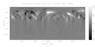
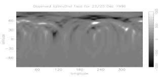
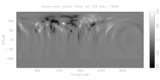
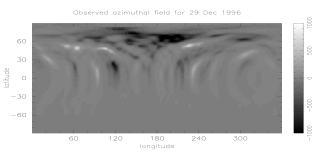
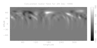
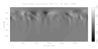
Figure 3: This diagram shows the azimuthal and radial components of the field in 1996. The top row gives the observed radial (left) and azimuthal (right) fields for Dec 23/25. The middle row gives the observed radial (left) and azimuthal (right) fields for Dec 29. The bottom row gives the calculated radial (left) and azimuthal (right) fields for Dec 29, assuming that $\eta$=450km²s^-1

The third stage is to take the evolved coefficients $B_{lm}$,$A_{lm}$ and $J_{lm}$ and the associated Legendre functions $P_{lm}$ and calculate the three components of the magnetic field- $B_{r}$ (radial), $B_{\phi}$ (azimuthal) and $B_{\theta}$ (meridional)- from them. These will be given by

$$B_{r}(r,\theta,\phi)=\sum_{l=1}^{N}\sum_{m=-l}^{l}B_{lm}P_{lm}(\theta)e^{im\phi}$$

$$B_{\theta}(r,\theta,\phi)=\sum_{l=1}^{N}\sum_{m=-l}^{l}\lambda_{l}\left[-A_{lm}(r)\frac{dP_{lm}}{d\theta}+iJ_{lm}\frac{mP_{lm}}{\sin\theta}\right]e^{im\phi}$$

$$B_{\phi}(r,\theta,\phi)=\sum_{l=1}^{N}\sum_{m=-l}^{l}\lambda_{l}\left[-A_{lm}(r)\frac{imP_{lm}}{\sin\theta}-J_{lm}\frac{dP_{lm}}{d\theta}\right]e^{im\phi}$$

where

$$\lambda_{l}=\frac{1}{l(l+1)}.$$

3 Results

As an initial consistency check we computed the evolution of the magnetic energy in the field at the surface, calculating the ratio of magnetic energy in the evolved case to the original.

A magnetic field has energy $B^{2}/2\mu$ per unit volume, so the total energy is

$$W=\int_{volume}\frac{B^{2}}{2\mu}dV$$

Fig 1 shows this for the 1998 field. The left-hand panel shows the degree of diffusive decay of the field energy over 30 days. The right-hand panel shows the increase in energy that would occur in the absence of diffusion, due to the winding-up of the field by the differential rotation.

3.1 Long-term evolution of the surface field

We took the observed field for the 1995 and 1998 observations and evolved it over 30 days according to the induction equation (4). This allowed us to study the variation with time of the cross-correlation of the radial component observed on the first night with that calculated for subsequent nights (Fig 2). We chose two latitudes: 30 and 60°north. The results for 1998 are qualitatively similar. In all cases, the cross-correlation function decays by approximately 10% over 30 days. Although choosing a higher value for the diffusivity does cause a more rapid decay of the field and hence a faster decay of the cross-correlation function, it is still not enough to explain the complete lack of correlation found by ? for He699. It appears that for AB Doradûs, if diffusion and differential rotation were the only processes causing the field to evolve, that even after one month there should still be a good correlation.

Figure 4: The peak amplitude of the cross-correlation function between the observed and calculated radial (left) and azimuthal (right) fields for latitudes between 0 and 80°north for 1996 Dec 29. The solid line represents $\eta=250$km²s^-1, the dotted line $\eta=350$km²s^-1, the dashed line $\eta=450$km²s^-1 and the dot-dash line $\eta=550$km²s^-1.

Figure 5: The peak amplitude of the cross-correlation function between the observed and calculated radial (left) and azimuthal (right) fields for latitudes between 0 and 80°north for 1996 Dec 29 with $\eta=450$km²s^-1. The solid line is with the differential rotation, and the dotted line is without the differential rotation.

3.2 Short-term evolution

For comparison, we can look at the field evolution over a much shorter period of time. This has the advantage that we can compare our results with the observed evolution of the field during a single observing run. Here we use data from the 1996 run, in which we secured two sets of magnetic maps, separated by 5 nights (Fig. 3). Our aim is to determine whether the observed magnetic elements retain their identities over a period of 5 nights in the presence of diffusion and differential rotation.

We began by investigating the effect of varying the diffusivity. We evolved the 1996 Dec 23/25 field forward in time using various values of the diffusion coefficient. In each case we cross-correlated the resulting radial field map with the observed radial field for Dec 29 (Fig 4). We ensured that the cross-correlation only involved those longitudes that were well-observed, viz. 18-180°(?). The cross-correlation function was computed for each of a set of latitudes between 0 and 80°in the visible hemisphere, and the amplitude of the strongest peak in the ccf at each latitude is plotted in Fig. 4. It can be seen that the five-day span of these observations is too short for differences in the value chosen for diffusivity to have much effect.

We also considered the case where the field was allowed to evolve under the influence of diffusion only, i.e. with the differential rotation switched off. We found that over the 5-day span of the 1996 December observations, the influence of the differential rotation was negligible (Fig. 5).

From these we see that altering the value of the diffusion and removing the differential rotation have little effect on the cross-correlation over 5 nights. We would need observations over a longer timescale, say a month, to be able to look for meaningful results.

4 The high-latitude azimuthal field

? demonstrated that the high-latitude azimuthal band of field was not reproduced by modelling the field as potential. Here we investigate whether the differential rotation could produce this band by taking the 1998 radial field map and adding in a cap of unipolar radial field extending from the pole to latitude 80°, well within the dark polar spot seen in the stellar surface-brightness map. An identical cap of opposite polarity was added to the unobservable hemisphere to conserve flux. We emphasize that the polarity and strength of the dark polar cap cannot be determined directly from the observations, since the low surface brightness and strong foreshortening suppress the Zeeman signal from this part of the star. For each of a range of plausible polar field strengths and polarities we evolved the field forward in time for 5 days, then compared the mean value of $B_{\phi}$ at each latitude with the observed value.

We see from Fig. 6 that a high-latitude azimuthal band of negative polarity is produced when we shear the image at the observed differential rotation rate with a polar cap having $B_{r}<0$ and vice versa. The results confirm that the observed differential rotation is capable of producing a high-latitude negative azimuthal band, as is seen in the observations from all three observing seasons (Fig. 7). This predicts that the magnetic polarity of the dark polar region was predominantly negative in all three seasons.

The latitude of the maximum in $B_{\phi}$ occurs at the edge of the imposed unipolar cap in Fig. 6. The azimuthal field is localised here because most field lines originating in the north polar cap are connected to high northern latitudes just outside the cap. The direction of these field lines depends strongly upon the distribution of radial field at mid to high latitudes. Changing the strength of the polar cap has little effect on field lines at low latitude. This corresponds to our result that $\sum B_{\phi}$ varies little at low latitude as the strength of the cap is altered (as seen in Fig 6).

The observed azimuthal band plotted in Fig. 7 is more diffuse than the model, having a broader peak between latitudes 65°and 80°in all three seasons’ data. This corresponds roughly to the edge of the dark polar region, which extends to latitude 70°or so. The breadth of the peak suggests a more gradual fall-off in the polar field than we imposed on the model. The apparent decrease in field strength at latitudes above 70°can probably be ascribed to suppression of the Zeeman signal within the dark polar region.

The strength of the azimuthal field after only 5 nights is substantially less than that observed. This is not surprising, since the timescale on which shear can generate an azimuthal field with a strength comparable to the radial and meridional field will be of order the equator-pole lap time of 110 days. The diffusion time for length scales comparable to the size of the individual magnetic regions in the images is also of this order. Once an equilibrium is established between diffusion and differential rotation, we would expect the azimuthal field strength to be an order of magnitude greater than that produced after 5 days, in agreement with the observations. On a 100-day timescale, however, we expect the picture to be complicated further by the emergence of new flux, making a direct comparison with the observations problematic.

Figure 6: Azimuthally-averaged values of $B_{\phi}$ as a function of latitude computed from the 1998 data, evolved for 5 nights with $\eta=250$km²s^-1 and with different values of the polar field. The solid line is the case where the polar field is set to 0G, the dotted line where it is set to +1000G, the dashed line where it is set to -1000G, the dash-dot line where it is set to +4000G and the long-dashed line where it is set to -4000G.

Figure 7: Azimuthally-averaged values of $B_{\phi}$ as a function of latitude in the observed field maps for 1995 (solid line), 1996 Dec 23/25 (dotted line) and 1998 (dashed line).

5 Conclusions

We have modelled the evolution of the magnetic field of AB Doradûs due to the effects of differential rotation and diffusion. We use as a starting point the Zeeman Doppler images obtained on three consecutive years and assume that the field is initially potential, but evolves away from this state as a function of time.

Over a timescale of 20 to 30 days we have determined, as a function of time, the cross-correlation of our model radial magnetic field with the observed radial component on the first night. We find that over one month, the cross-correlation function decays by about 10%. Observations of He699 by ? show however that cross-correlating the observed spot distributions over this timescale gives much more rapid decrease of the cross-correlation function. This result suggests that the evolution of AB Doradûs’s surface magnetic field is not governed solely by diffusion and differential rotation. We conclude that these results are more likely to be due to the effects of flux emergence changing the spot distribution than the effects of diffusion or differential rotation.

This result is independent of the assumed degree of field diffusion. We have compared the effects of values of $\eta$ ranging from 250 to 450 km²s^-1 and found the results to be qualitatively the same. The presence of some diffusion is of course necessary (and we have confirmed that the magnetic energy grows monotonically with time in the absence of diffusion). The exact value of $\eta$ seems however to have little effect on the five-day timescale of a typical observing run. Since diffusion has little effect on the flux distribution, the differential rotation acts simply to advect the field. Consequently, although at each latitude the peak of the cross-correlation function may be at a different longitude (?), its actual value is virtually unchanged by the effects of differential rotation.

We have also compared the radial and azimuthal magnetic fields generated by our model over 5 nights with those obtained from Zeeman Doppler images on 1996 Dec 23/25 and 29, and found the agreement to be excellent. The evolution of the azimuthal field is of particular interest with regard to the band of high latitude unidirectional azimuthal field seen in the Zeeman-Doppler images. We have investigated whether the shearing effect of the differential rotation is sufficient to generate this band of field. The polarity of this band depends upon the sign of the radial field in the polar cap, whereas its strength depends on the competition between shear and diffusion. Since the diffusion timescale for resolvable features is comparable to the winding time, we expect the azimuthal field to attain a strength comparable to the radial and meridional field near the boundary of the polar cap, as is indeed observed. Our results suggest that the differential rotation could play a major part in the creation and preservation of a high latitude azimuthal band.

6 Acknowledgements

We would like to thank Drs. D. Mackay, A. van Ballegooijen and M. Ferreira for useful discussions and assistance during the course of this work. We also thank Drs. G. Hussain and L. Kitchatinov for their careful reading of the manuscript and offering comments. GRP acknowledges the support of a studentship from the University of St Andrews.

References

- Anders 1990 Anders G., 1990, Inf. Bull. Variable Stars, 3437
- Barnes et al. 1998 Barnes J. R., Collier Cameron A., Unruh Y. C., Donati J.-F., Hussain G. A. J., 1998, MNRAS, 299, 904
- Berger et al. 1998 Berger T. E., Löfdahl M. G., Shine R. A., Title A. M., 1998, ApJ, 506, 439
- Collier Cameron & Foing 1997 Collier Cameron A., Foing B. H., 1997, Observatory, 117, 218
- Collier Cameron & Robinson 1989a Collier Cameron A., Robinson R. D., 1989a, MNRAS, 236, 57
- Collier Cameron & Robinson 1989b Collier Cameron A., Robinson R. D., 1989b, MNRAS, 238, 657
- Collier Cameron & Unruh 1994 Collier Cameron A., Unruh Y. C., 1994, MNRAS, 269, 814
- Collier Cameron et al. 1988 Collier Cameron A., Bedford D. K., Rucinski S. M., Vilhu O., White N. E., 1988, MNRAS, 231, 131
- Collier Cameron et al. 1990 Collier Cameron A., Duncan D. K., Ehrenfreund P., Foing B. H., Kuntz K. D., Penston M. V., Robinson R. D., Soderblom D. R., 1990, MNRAS, 247, 415
- Collier Cameron et al. 1999 Collier Cameron A. et al., 1999, MNRAS, 308, 493
- Collier Cameron 1995 Collier Cameron A., 1995, MNRAS, 275, 534
- Donati & Collier Cameron 1997 Donati J.-F., Collier Cameron A., 1997, MNRAS, 291, 1
- Donati et al. 1999 Donati J.-F., Collier Cameron A., Hussain G. A. J., Semel M., 1999, MNRAS, 302, 437
- Hussain, Jardine & Collier Cameron 2001 Hussain G. A. J., Jardine M., Collier Cameron A., 2001, MNRAS, 322, 681
- Hussain, van Ballegooijen & Jardine 2001 Hussain G. A. J., van Ballegooijen A., Jardine M., 2001, in Twelfh Cambridge Workshop on Cool Stars, Stellar Systems, and the Sun. ASP Conference Series, San Francisco, In press
- Innis et al. 1988 Innis J. L., Thompson K., Coates D. W., Lloyd Evans T., 1988, MNRAS, 235, 1411
- Jardine & Ferreira 1996 Jardine M., Ferreira J. M. T. S., 1996, Astrophysical Letters and Communications, 34, 101
- Jardine et al. 1999 Jardine M., Barnes J., Donati J.-F., Collier Cameron A., 1999, MNRAS, 305, L35
- Kitchatinov & Rüdiger 1999 Kitchatinov L., Rüdiger G., 1999, A&A, 344, 911
- Kürster et al. 1997 Kürster M., Schmitt J. H. M. M., Cutispoto G., Dennerl K., 1997, A&A, 320, 831
- Kürster, Schmitt & Cutispoto 1994 Kürster M., Schmitt J. H. M. M., Cutispoto G., 1994, A&A, 289, 899
- Lim et al. 1994 Lim J., White S. M., Nelson G. J., Benz A. O., 1994, ApJ, 430, 332
- Maggio et al. 2000 Maggio A., Pallavicini R., Reale F., Tagliaferri G., 2000, A&A, 356, 627
- Pakull 1981 Pakull M. W., 1981, A&A, 104, 33
- Rucinski 1982 Rucinski S. M., 1982, Inf. Bull. Variable Stars, 2203
- Schatten, Wilcox & Ness 1969 Schatten K., Wilcox J., Ness N., 1969, Solar Phys., 6, 442
- Schmitt, Cutispoto & Krautter 1998 Schmitt J. H. M. M., Cutispoto G., Krautter J., 1998, ApJ, 500, L25
- Unruh, Collier Cameron & Cutispoto 1995 Unruh Y. C., Collier Cameron A., Cutispoto G., 1995, MNRAS, 277, 1145
- van Ballegooijen, Cartledge & Priest 1998 van Ballegooijen A., Cartledge N., Priest E., 1998, ApJ, 501, 866