A Bayesian non-parametric method to detect clusters in Planck data.

Abstract

We show how one may expect a significant number of SZ detections in future Planck data without any of the typical assumptions needed in present component separation methods, such as about the power spectrum or the frequency dependence of any of the components, circular symmetry or a typical scale for the clusters. We reduce the background by subtracting an estimate of the point sources, dust and CMB. The final SZE map is estimated in Fourier space. The catalogue of returned clusters is complete above flux $\approx 200$ mJy (353 GHz) while the lowest flux reached by our method is $\approx 70$ mJy (353 GHz). We predict a large number of detections ($\sim 9000$) in 4/5 of the sky. This large number of SZ detections will allow a robust and consistent analysis of the evolution of the cluster population with redshift and will have important implications for determining the best cosmological model.

1 Introduction

The distortion in the radiation intensity of CMB photons produced when they traverse the hot intracluster plasma in the direction of a galaxy cluster (Sunyaev-Zel’dovich effect, Sunyaev & Zel’dovich 1972) is one of the most promising effects being studied for exploring cosmological models. In recent years, several groups have been working on the detection of the SZE and many detections have been reported (e.g. Birkinshaw et al. 1984, Carlstrom et al. 1996, Pointecouteau et al. 2001). The SZE is growing in interest as the number of experiments and their quality is increasing. The number of experiments devoted to these kind of observations, as well as their unprecedented quality, will allow a variety of analyses which, combining the SZ data with other data or alone, could be applied to the study of the intracluster media, its origin and evolution; the abundance of galaxy clusters and its important cosmological implications; the determination of the cosmological distances to the most distant galaxy clusters, etc. One of these experiments is the approved Planck satellite (scheduled launch in 2007). This satellite will observe the full sky at mm frequencies (30 GHz $<\nu<$ 857 GHz) and with resolutions ranging from $FWHM=30$ arcmin to $FWHM=5$ arcmin. Previous studies have shown that this satellite will produce a full sky cluster catalogue with about $5000-50000$ clusters; the final number depending on the cosmological model, the Planck effective sensitivity and the method used to identify the different component contributions. This paper will be focused on this last point.

Recent proposed component separation methods, Wiener filter (WF, Tegmark & Efstathiou 1996, Bouchet et al. 1997), maximum entropy (MEM, Hobson et al. 1998, 1999), fast independent component analysis (FastICA, Maino et al. 2001), mexican hat wavelet analysis (MHW, Cayón et al. 2000, Vielva et al. 2001a), and adaptive filter analysis (AFA, Tegmark & de Oliveira-Costa 1998, Sanz et al. 2001), are being tested in order to define a well established method to perform the component separation on the Planck data. However, it will be extremely difficult to define the best method since some methods will work better than others under certain circumstances, and it will not be surprising if, at the end, the final component separation method results in a combination of a variety of methods (e.g. MEM $+$ MHW, Vielva et al. 2001b).

Some methods try to separate all the components simultaneously. To do this in an effective way, some a priori information is needed. Commonly, the power spectrum of several (if not all) components and the frequency dependence of the components must be given (WF, MEM). Another typical assumption is that all the components are independent and non-Gaussian except maybe one, the CMB (FastICA).
In the case that the assumed information is close enough to reality, all of these methods work very well. On the other hand, if the a priori information is wrong, the result of the component separation will be biased with respect to the underlying real signal. This could have important consequences on the analysis of the final data maps. One of the risks in the simultaneous all component separation methods is then that an error in the estimation of one of the components must be compensated by an error in one (if not all) of the other components due to the constraint that the sum of all the recovered components must equal the data.

This problem can be partially reduced by using single component separation methods like the MHW or AFA which have been successfully applied to the separation of point sources (Cayón et al. 2000, Vielva et al. 2001a) and the SZ effect (Herranz et al. 2002a,b). These methods have the advantage, over the previous ones, that they do not need to assume anything about the Galactic components or the CMB. The information they need is taken directly from the data (the power spectrum of the background and the beam shape). The only thing they have to assume is a scale and the circular symmetry of the source. In the MHW technique applied to detect point sources, the optimal scale can be obtained from the background and the beam scale. In this sense, the analysis of the point sources based on the MHW technique is very robust since all the assumptions are taken from the data. When the AFA is applied to the detection of the SZ effect, a prior knowledge of the scale and shape (asymmetry) of the clusters is needed (Sanz et al. 2001). This problem can be overcome by applying the filter at different scales (Herranz et al. 2002a,b). The problem of asymmetry in the resolved clusters can only be solved by rotating an axis-asymmetric filter which will reduce significantly the speed of the algorithm.

In this work we propose an alternative method which can be applied to the detection of the SZ signal on the future Planck data. The main points of our method are the following:

$\bullet$ We consider a Bayesian and non-parametric method without prior knowledge about the power spectrum of any of the components. We will show how the method allows us to include information about the power spectrum of the SZE component. However the final result will not depend significantly on the particular choice of this power spectrum and arbitrary power spectra can be considered provided they obey some general rules.

$\bullet$ The method is easy to implement and fast since it is a non-iterative method and all the equations are solved in Fourier space mode by mode.

$\bullet$ We do not need any prior knowledge about the frequency dependence of the components other than the SZ, and, obviously, the CMB. We only require that we have at least one channel which is clearly dominated by dust. However, results from BOOMERANG and IRAS suggest that the 857 GHz channel in Planck will be dominated by dust.

$\bullet$ The method works for any kind of shapes and sizes of the galaxy clusters.

$\bullet$ The method uses all the information available (all the channels).

As mentioned in the third point, we will assume only knowledge of the frequency dependence of the SZ effect (see fig. 2). This is a well established assumption as the physic of the SZ effect is very well known. We would like to remark that, although in this work we will assume only the non-relativistic corrections, our conclusions could be extended to include the relativistic corrections (provided the temperature of the cluster is known). We also did not consider the kinetic contribution to the SZ effect since it is of order 30 times smaller than the thermal part. However, this component could be estimated (in some clusters) as the residuals after the thermal contribution has been determined.

The structure of the paper is the following. In section 2 we present the Planck simulations that have been used to test the method. We describe the method and the way it is implemented in section 3. We apply the method to the realistic Planck simulations and show the results in section 4. Finally, we compare briefly with other methods in section 5. The possibilities of the recovered SZE map are also highlighted in this section.

2 Data set: realistic Planck simulations

Figure 1: Initial simulated maps at the Planck frequency channels. They contain: CMB, thermal Sunyaev-Zel’dovich effect, thermal dust emission, free-free, synchrotron, spinning dust, point source emission and instrumental Gaussian white noise. In this plot and in the next ones, the color table is in units of $\Delta T/T$.

In order to check the power of the method, we have performed realistic Planck simulations. The simulations are realistic in the sense that they include all the main features of the Planck satellite such as the corresponding noise level in each channel, pixel size and antenna beam (see table 1). They are also realistic in the sense that all the components (CMB, Galactic components, extra-galactic point sources and SZ) were simulated including the latest information we have about these components. The simulations were done in patches of the sky of $12.8^{\circ}\times 12.8^{\circ}$ although the method can be easily extended to include all the sphere. For the sake of simplicity, we will not include the effect of the bandwidths in our simulations although there is no problem if the bandwidths have to be included. Therefore, we will simulate the different maps only at the central frequency of the Planck channels.

The CMB simulation has been done for a spatially flat $\Lambda$CDM Universe with $\Omega_{m}=0.3$ and $\Omega_{\Lambda}=0.7$, using the $C_{l}$’s generated with the CMBFAST code (Seljak & Zaldarriaga, 1996). It is a Gaussian realization.

The thermal Sunyaev-Zel’dovich (SZ) effect simulation was made for the same cosmological model. The cluster population was modeled using Press-Schechter (Press & Schechter 1974) with a Poissonian distribution in the angular coordinates of the 2D map, $\theta$ and $\phi$. The model was selected by fitting the cluster population as a function of $z$ to several X-ray and optical cluster data sets. In that fit we obtained certain values for the cosmological parameters as well as an estimate for the parameters involved in the cluster scaling relations $T-M$ and $L_{x}-T$ (see Diego et al. 2001a for a discussion).

The extra-galactic point source simulation was performed following the model of Toffolatti et al. 1998 assuming the cosmological model indicated above. The simulation include radio flat-spectrum and infrared sources. VLA and IRAS catalogues were used to fix the model. The predictions obtained with this model are compatible with ISO and SCUBA data (see the above paper for more details).

Frequency	FWHM	Pixel size	$\sigma_{noise}$	CMB	TDust	FF	Synch.	SDust	PS	SZ
(GHz)	(arcmin)	(arcmin)	$(10^{-6})$	$(10^{-6})$	$(10^{-6})$	$(10^{-6})$	$(10^{-6})$	$(10^{-6})$	$(10^{-6})$	$(10^{-6})$
857	5.0	1.5	22211.10	42.70	140000.00	39.60	17.30	0.00	11400.00	19.60
545	5.0	1.5	489.51	42.70	1090.00	1.10	0.58	0.00	92.80	9.86
353	5.0	1.5	47.95	42.70	58.50	0.23	0.15	0.00	5.16	3.93
217	5.5	1.5	15.78	42.50	7.53	0.16	0.12	0.00	1.57	0.03
143	8.0	1.5	10.66	41.0	2.33	0.21	0.20	0.00	1.91	1.40
100 (HFI)	10.7	3.0	6.07	39.40	1.07	0.36	0.39	0.00	2.90	1.65
100 (LFI)	10.0	3.0	14.32	39.8	1.06	0.35	0.39	0.00	3.11	1.73
70	14.0	3.0	16.81	37.6	0.54	0.67	0.87	0.27	4.00	1.59
44	23.0	6.0	6.79	33.2	0.24	1.64	2.65	3.17	5.82	1.16
30	33.0	6.0	8.80	29.3	0.12	3.56	6.87	8.94	8.35	0.89

Table 1: Experimental constrains and simulation characteristics at the 10 Planck channels. The antenna FWHM is given in column 2 for the different frequencies (a Gaussian pattern is assumed in the HFI and LFI channels). Characteristic pixel sizes are shown in column 3. The fourth column contains information about the instrumental noise level, in $\Delta T/T$ per pixel. In columns 5 to 11 we show the dispersion of the simulated components (CMB, thermal dust emission, free-free, synchrotron, spinning dust, point sources and Sunyaev-Zel’dovich effect respectively) in $\Delta T/T$ per pixel, after beam convolution.

We have simulated four different Galactic emission sources: thermal dust, free-free, synchrotron and spinning dust.

The thermal dust emission was simulated using the data and the model provided by Finkbeiner et al. (1999). This model assumes that dust emission is due to two grey bodies: a hot one with a dust temperature of ${T_{D}}^{hot}\simeq 16.2K$ and an emissivity $\alpha^{hot}\simeq 2.70$, and a cold one with a ${T_{D}}^{cold}\simeq 9.4K$, and an $\alpha^{cold}\simeq 1.67$. These quantities are mean values. The temperatures and emissivities change from point to point. An exhaustive description of the model is given in their paper, where the authors combined data from DIRBE, IRAS and FIRAS to fit the dust emission at high frequencies (500 GHz to 3000 GHz). We will use their best fitting model in this work.

The distribution of free-free emission is poorly known. Present experiments such as the H-$\alpha$ Sky Survey and the WHAM project will provide maps of $H_{\alpha}$ emission that could be used as a template. In this work, we have created the free-free template correlated with the dust emission as proposed in Bouchet, Gispert & Puget (1996). The frequency dependence of the free-free emission is assumed to change as $I_{\nu}\propto{\nu}^{-0.16}$, and is normalized to give an RMS temperature fluctuation of $6.2\mu K$ at 53 GHz.

Synchrotron emission simulations have been done using the all sky template provided by P. Fosalba and G. Giardino in the FTP site: ftp://astro.estec.esa.nl. This map is an extrapolation of the 408 MHz radio map of Haslam et al. 1982, from the original $1^{\circ}$ resolution to a resolution of about $5$ arcmin. The additional small-scale structure is assumed to have a power-law power spectrum with an exponent of $-3$. We have done an additional extrapolation to the smallest scale ($1.5$ arcmin) with the same power-law. We also include in our simulations the information on the changes of spectral index as a function of electron density in the Galaxy. This template has been done combining the Haslam map with the Jonas et al. 1998 at 2326 MHz and with the Reich & Reich 1986 map at 1420 MHz, and can be found in the previous FTP site.

We have also taken into account possible galactic emission due to spinning grains of dust, proposed by Draine & Lazarian 1998. This component could be important at the lowest frequencies of the Planck channels (30 and 44 GHz) in the outskirts of the galactic plane.

3 A method in 2 steps

In this section, we describe our proposed new method to estimate the SZ thermal contribution to the mm data in the 10 Planck channels. A detailed description of the mission can be found in the official Planck web address http://astro.estec.esa.nl/Planck/.

The expected sensitivity of Planck to detect the SZ effect in each one of its 10 channels is shown in Fig. 2 as vertical lines centered in each one of the central frequencies. The amplitude of this lines is proportional to $f(\nu)/\sigma(\nu)$ where $\sigma(\nu)$ is the sensitivity per resolution element of the channel at frequency $\nu$. The factor $f(\nu)$ is just the frequency dependence of the thermal SZ effect:

$$\frac{\Delta T}{T}(\nu)=f(\nu)y_{c}$$ (1)

where $y_{c}$ is the Compton parameter, $T$ is the thermodynamic mean temperature of the CMB ($T\approx 2.73$ K) and $\Delta T$ is the change in the thermodynamic CMB temperature induced by the SZE. The thermodynamic temperature is related to the intensity, $I$, through:

$$T(\mu K)\approx\frac{1}{24.8}{\Big{(}{\frac{\sinh{(x/2)}}{x^{2}}}\Big{)}^{2}}I(Jy~{}sr^{-1})$$ (2)

where $x\approx\nu/56.8$ GHz.

Figure 2: $f(\nu)$ factor appearing in eqn. (1). The vertical lines are proportional to the signal-to-noise ratio for the SZE expected in each one of the Planck channels. Planck frequencies are centered at 30, 44, 70, 100 (LFI & HFI), 143, 217, 353, 545 and 857 GHz. The planned bandwidths for Planck (not considered in this work) are $\delta\nu/\nu=0.2$ for the LFI (30-100 GHz) and $\delta\nu/\nu=0.25$ for the HFI (100-857 GHz). The channels at 217 and 857 GHz show a tiny S/N ratio. At 100 GHz there are two channels; LFI channel (solid line) and HFI channel (dotted line).

¿From figure 2 it can be seen that the best channels are those between 100 and 353 GHz. Although the channel at 217 GHz does not seem to be relevant, it is in fact one of the most important to detect the SZ effect since at this frequency the thermal SZ effect is expected to be negligible. The other channel that does not seem to be relevant is the highest one at 857 GHz which is expected to be completely dominated by the dust emission coming from our Galaxy (see Table 1). However, as we will see later, both channels will play a crucial role in our method.
The method is in fact divided in two main steps.

In the first step -map cleaning- we reduce the contribution of certain components (point sources, dust and CMB) under the assumption that point sources are unresolved, the thermal dust emission is, at different frequencies, the same spatial pattern times a parameter which depends on the frequency and the CMB is frequency-independent. This process will increase the noise level of the maps but will increase as well the S/N ratio of the SZE signal.

In the second step -Bayesian approach- we develop a method to search for the Compton parameter in each pixel responsible of the SZ signature in our clean maps. We will define our approach in terms of Bayes’ theorem.

3.1 Map cleaning

A typical CMB experiment will measure not only the CMB signal but also other additional components such as the Galaxy (synchrotron and free-free emission at low frequencies and dust emission at high frequencies), extra-galactic sources which for the Planck resolution will appear as unresolved point sources, and finally the SZE. The integrated contribution of these components is detected with an antenna having a given response (different at each channel). In addition we have to include the noise of our detectors which also will depend on the frequency (channel). The final signal at a given frequency will be therefore:

$$\frac{\Delta T}{T}(\nu,\vec{x})=A\otimes\sum_{i}\frac{\Delta T_{i}}{T}(\nu,\vec{x})+\frac{\Delta T(\nu,\vec{x})^{N}}{T}$$ (3)

where $\sum_{i}$ is a sum over all the components (CMB, Galactic components, extra-galactic point sources and SZE) and $\Delta T(\nu,\vec{x})^{N}/T$ contains the contribution due to the noise in the receivers. We have considered a white Gaussian uniform noise. In a real situation, the noise will not be uniformly distributed. This effect is minimized when taking small sky patches.

$\Delta T/T(\nu,\vec{x})$ denotes the measured temperature of the sky minus the temperature of the CMB ($T_{CMB}\approx 2.73$ K) divided by $T_{CMB}$. The term $A\otimes$ denotes the convolution with the antenna. There should be an additional term in the previous equation to account for the frequency response of our experiment which is not a delta function at the frequency $\nu$. Therefore a real experiment will measure $\Delta T/T(\nu_{1}-\nu_{2},\vec{x})$. This is just another convolution of Eq. 3 with the frequency response of the instrument centered at the frequency $\nu$. For simplicity we will not consider the bandwidth in our calculations although it could easily be included.
By looking at Eq. 3, it is easy to understand the complexity of the component separation problem. In this work we are only interested in one of these components, the SZE. The complexity of estimating that component could be reduced if we can subtract first, or at least reduce significantly, the contribution of some of the other components in Eq. 3. By reducing the contribution of some of the dominant components, the S/N ratio of the SZ signal can be increased, since the smaller the background the better our determination of the signal. But one should be careful in the process of subtracting some of the other components since we do not want to remove any SZE signal.
There are several components which can be easily subtracted from the Planck data (or at least reduce their contribution to the background) without subtracting any significant thermal SZE signal.

Point sources.

The point source contribution is expected to be specially relevant at the highest Planck frequency channels. The point source emission at these high frequencies is due to infrared sources. At the lowest Planck frequencies, the point source emission is mainly due to radio flat-spectrum AGNs. The knowledge of the point source emission at the intermediate Planck channels is really poor. In fact, the determination of the point source emission at these frequencies is one of the challenges of the Planck mission.

The detection of the point source emission is a special issue for the component separation problem. There are two main differences between this emission and the other foregrounds. First, the frequency behaviour can change significantly from one point source to another. Second, the point source emission has a typical scale: the beam width. These properties suggest that common component separation methods such as MEM, WF or neural networks are not the best techniques to detect the point source emission.

We have applied the MHW technique first described in Cayón et al. (2000) and later extended in Vielva et al. (2001a). Wavelets are a powerful tool to detect point sources. When a signal with a characteristic scale is analyzed with a wavelet adapted to its shape, its wavelet coefficients are amplified with respect to the background coefficients. This amplification occurs at scales around the characteristic scale (Cayón et al. 2000). We can increase the number of detections by looking at the scale which maximizes the amplification (Vielva et al. 2001a). This optimal scale can be determined directly from the data. Therefore, there is no need for assumptions either about the nature or characteristics of the underlying signals (e.g. spectral behaviors, power spectra, pdf, etc). The optimal pseudo-filter for the detection of point sources which are convolved with a Gaussian beam (at least for 2D images with a power spectrum described by $C_{l}\sim l^{-2}$ around the point source scale) is the MHW (Sanz et al. 2001). A detailed description of the point source detection algorithm can be found in Vielva et al. (2001a). Here we will just describe the main steps.
First, we search for the optimal MHW scale that maximizes the amplification (source amplitude ratio, in dispersion units, between wavelet and real spaces) at each frequency. As we mentioned above, all the information we need is in the data itself. Basically, the function that must be maximized is:

$$\textrm{$\mathcal{A}$}(R)\propto\int{dkkP(k)|\widehat{\psi}(Rk)|^{2}}$$ (4)

where $P(k)$ is the power spectrum of the map, $|\widehat{\psi}(Rk)|$ is the Fourier transform of the MHW and R is the MHW scale. Once the optimal scale is determined, we select certain point source candidates (those maxima at the MHW optimal scale map that are above a certain level). The next step is to get the amplitude of those point source candidates. The amplitude estimation is done by fitting the theoretical dependence of the point source wavelet coefficient with the MHW scale. Then, we convolve the map with three additional MHW (at adjacent scales to the optimal one) and we fit the obtained coefficients to the theoretical curve:

$$\frac{w(R)}{R}=2\sqrt{2\pi}B\frac{(R/\sigma_{a})^{2}}{(1+(R/\sigma_{a})^{2})^{2}}$$ (5)

where $w(R)$ is the wavelet coefficient at the scale $R$, $\sigma_{a}$ is the beam dispersion and $B$ is the PS amplitude (the parameter to be determined). After this, a detection criterion is applied to select the real point sources (see Vielva et al. 2001a) and those point sources are subtracted from the original data.

Dust.

The second contribution which can be easily subtracted is the thermal dust emission. This emission can be important at frequencies above $\approx 100$ GHz. At frequencies of $\approx$ 350 GHz, dust starts to dominate over the other components and its contribution is even more important at higher frequencies. The Planck channel at 857 GHz is expected to be completely dominated by dust (as suggested by the BOOMERANG and IRAS results). This map can therefore be used as a spatial pattern of the distribution of dust in our Galaxy. The only thing we need to know to subtract the dust from the other channels, is the frequency dependence of the dust. However, since we do not want to assume any frequency dependence (and this is unknown in the range of frequencies of Planck) we need to look for other alternatives to subtract the dust.

Essentially, our method to subtract the dust emission looks for a parameter, $\alpha(\nu)$, which depends on the frequency and is such that the difference

$$\xi(\nu,\vec{x})=M(\nu,\vec{x})-\alpha(\nu)M(857,\vec{x})$$ (6)

has a minimum dust contribution in terms of the variance. $M(\nu,\vec{x})$ denotes the Planck map at frequency $\nu$ to which we want to subtract the dust, $M(857,\vec{x})$ is the map at 857 GHz (dust map) and $\xi(\nu,\vec{x})$ is the new map at frequency $\nu$ after dust subtraction. Then, the $\alpha(\nu)$ parameter is determined by imposing that the variance of the residual map $\xi(\nu,\vec{x})$ must be a minimum. If we write down the expression for this variance:

$${\sigma(\nu)^{2}}_{R}\propto\int\xi(\nu,\vec{x})^{2}d\vec{x}=\int(M(\nu,\vec{x})-\alpha(\nu)M(857,\vec{x}))^{2}d\vec{x}$$ (7)

and now we require that the derivative of ${\sigma(\nu)^{2}}_{R}$ with respect to $\alpha(\nu)$ must be $0$, we finally find:

$$\alpha(\nu)=\frac{\int M(\nu,\vec{x})M(857,\vec{x})d\vec{x}}{\int M(857,\vec{x})^{2}d\vec{x}}$$ (8)

where $\int d\vec{x}$ refers to an integral in real space over all the pixels of the map. At the end, what we obtain is a value for $\alpha(\nu)$ which is different for each frequency. The values of $\alpha(\nu)$ should approach the real frequency dependence of the dust at these frequencies. It is important to remark that by subtracting the dust with this method we are not perfectly subtracting this component. This method is assuming that the dust has the same frequency dependence in the analyzed sky patch which is a good assumption for small regions of the sky. However, as it will be noted in section 4, this approach has been proved to be successful with our simulations where we have really considered a varying spectral index and grain temperature for the dust emission. We have computed the spatial distribution of the spectral index on our simulated dust maps. We found that is nearly constant with a dispersion of about $3\%$.
We would like to note that our method to subtract the dust is nothing less but a Wiener Filter since we are looking for a linear operation on the maps such that the variance of the residual is minimum. This is just the general definition for Wiener filter (e.g Zaroubi et al. 1995).

CMB.

CMB is the last component that can be subtracted easily. Since the $\Delta T/T$ distortion in the CMB map is independent of the frequency, a good approach for the contribution of the CMB in each of the channels can be obtained by filtering a given CMB-dominated channel to the resolution of the other channels. The selection of the optimal channel to be filtered is easy if we want to increase the S/N ratio of the SZ effect. The channel at 217 is expected to have a negligible contribution to the thermal SZ effect while the CMB component dominates over the other ones. Furthermore, this channel has a resolution (FWHM = 5.5 arcmin) very close to the best Planck resolution (FWHM = 5 arcmin). Moreover, this channel has a low noise level (although it is not the best channel in terms of the noise level).

Therefore our first step in cleaning the maps of the CMB contribution is to filter the high frequency channels with FWHM = 5 arcmin to the resolution of the channel at 217 GHz (FWHM = 5.5 arcmin) (FWHM-Filter = $\sqrt{5.5^{2}-5^{2}}$) where we have assumed that the beam can be well described by a Gaussian. Then, the channel at 217 GHz is subtracted from the filtered channels. We repeat the process with the channels at frequencies below 217 GHz but in this case we have to filter the 217 GHz channel to the resolution of the other channels since in this case the channels below 217 GHz have a FWHM larger than 5.5 arcmin.

It is important to keep the previous order (PS, dust and CMB). Point sources should be extracted first (at least in the channel at 857 GHz) since the frequency dependence of the point sources will be in general different to the frequency dependence of the dust in our Galaxy. Therefore if we subtract the 857 GHz map including the point sources in that map we are assuming that these point sources have the frequency dependence of our Galaxy, which is wrong. Then we should subtract the dust prior to the subtraction of the CMB (217 GHZ map) since we need to reduce the dust contribution in the 217 GHz map before subtracting this channel from the others.

We have to point out that, in the process of subtracting the components, we have increased the S/N ratio for the SZE but we have also increased the noise level. First, when subtracting the dust, we are adding the noise level of the 857 GHz map times the constant $\alpha(\nu)$ to the other maps. This process does not increase the noise level very much in the channels below 300 GHz. At these frequencies the CMB contribution starts to dominate over the thermal dust and the value of $\alpha(\nu)$ is, therefore, very small. Hence, the noise contribution is small as well.

Since the S/N ratio of the dust in the 857 GHz map is high and the value $\alpha(\nu)$ is small at these low frequencies, then, the dust is subtracted without increasing the noise level too much in the low frequency channels. Furthermore, since the 857 GHz channel must be filtered, this process decreases the noise level even more.

The increase in the noise level due to the CMB subtraction is more important in those channels where the resolution is closer to the one at 217 GHz (143, 353, and 545 GHz channels) and is less important in the other channels. This is because we have to filter the maps to the resolution of the lowest resolution channel. Hence, if the filter has a large FWHM (FWHM-Filter = $(FWHM_{\nu}^{2}-FWHM_{217}^{2})^{1/2}$), then the noise is smoothed over the large scale of the filter. As a result, some channels (around 217 GHz) have increased their noise level significantly while others did not change the noise level too much.

3.2 The Bayesian approach

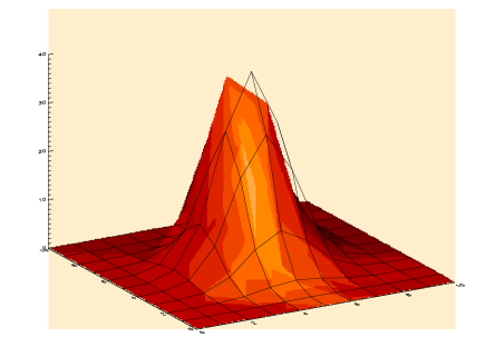
Figure 3: Probability distribution of the $y_{c}$ Fourier coefficients (coefficients on the ring with $|\vec{k}|=60$) for a simulated SZE map. The histogram is made in the Real-Imaginary plane ($X$ axis is the Real part of the Fourier coefficient, $Y$ axis is the Imaginary part and $Z$ axis is the number of Fourier coefficients with Real and Imaginary parts falling in the bin $(X,Y)$). Those coefficients with Real and Imaginary parts equal to 0 are in the center of the plane. The grid shows the pdf given by expression (13) with $P_{y_{c}}$ the power spectrum of the simulated map at $k=60$.

After the previous steps have been applied, we end up with maps where some point sources have been (partially) removed, the dust and CMB contributions have been reduced and the noise level has been increased (in the high frequency channels more than in the low frequency ones). The resulting maps are dominated by the residuals of the point source subtraction (low frequencies) and noise (all frequencies) while the SZE contribution appears to be more important at intermediate frequencies. Since we are only interested on the SZ effect and not on the residuals nor the noise we can consider them as a net residual, $\chi(\nu,\vec{x})$. Then the data, $d(\nu,\vec{x})$ (Eq. 3, hereinafter we write $d(\nu,\vec{x})$, instead of $\Delta T/T(\nu,\vec{x})$ for simplicity), can be rewritten as:

$$d(\nu,\vec{x}) = SZ(\nu,\vec{x})+\chi(\nu,\vec{x})$$ (9)

$$= A(\nu)\otimes(f(\nu)y_{c}(\vec{x}))+\chi(\nu,\vec{x})$$ (10)

where $f(\nu)$ is the known frequency dependence of the thermal SZ effect (see Fig. 2), $y_{c}(\vec{x})$ is the Compton parameter we want to determine and $\chi(\nu,\vec{x})$ includes the residuals (point source, galactic components and CMB) and the instrumental noise. Due to the antenna convolution, $A(\nu)\otimes$, it is easier to work in Fourier space where the modes can be solved independently (provided the data is a homogeneous and isotropic field). Therefore, the previous equation should be rather expressed in Fourier space

$$d_{\nu}(\vec{k})=A_{\nu}(\vec{k})f_{\nu}y_{c}(\vec{k})+\chi_{\nu}(\vec{k})$$ (11)

where each mode can now be solved independently. We have adopted the flat space approach which is good enough when the scale of the map is $<<1$ rad. Now we need some engine to search for the Fourier modes of the Compton parameter map which best resemble the real Fourier modes of the SZE in the data. We will use the Bayes theorem as such an engine:

$$P(y_{c}/d)\propto P(y_{c})P(d/y_{c})$$ (12)

where the only thing we need to do is to define the prior $P(y_{c})$ and the likelihood of the data $P(d/y_{c})$ and then look for the values of $y_{c}$ that maximize the posterior probability.

The prior.

The prior should account for the probability of having a given Compton parameter (in Fourier space). Since there is not enough real data to know what a real SZ map looks, this probability should be obtained from simulations of the SZ. We found that, in Fourier space, the probability of having a given $y_{c}$ at each $k-$mode is close to a Gaussian of the form:

$$P(y_{c})\propto exp(-{|y_{c}|}^{2}/P_{y_{c}}).$$ (13)

where $P_{y_{c}}$ is the power spectrum of the SZ map, at each $k-$mode.

We assume that the probability depends on $y_{c}$ through its module. This can be done due to the almost symmetric shape of the pdf of $y_{c}$ (see Fig.3). The real pdf is not exactly symmetric as can be appreciated in the figure. This means that the real pdf (in Fourier space) is not exactly a Gaussian which is in accordance with the non-Gaussian nature of the SZE in real space. However, the pdf of the modes of the SZE map in Fourier space (although not exactly Gaussian) can be approached by a Gaussian much better than the pdf of the SZE map in real space.
We found that the previous probability (equation 13) makes a reasonably good fit to the probability distribution of the $y_{c}$ at intermediate and large $\vec{k}$-modes (see Fig.3). At small $\vec{k}$-modes, Eq.(13) is still a reasonable approach although the small number of $y_{c}$ coefficients at these low $\vec{k}$-modes makes it difficult to have a (statistically) good enough probability distribution for $y_{c}$. Nevertheless, the interesting information containing the cluster contribution to the SZ effect is at intermediate $\vec{k}$-modes where Eq.(13) provides a reasonable approximation for the prior. The drawback of this approach is that we need to assume a given power spectrum for the SZ effect, $P_{y_{c}}$, in order to define the prior.

Figure 4: Power spectrum ($P_{yc}(k)$) for various simulations of the SZE. The three solid lines are the power spectrums of three simulations with $r_{v}/r_{c}=5,10,15$ and $\sigma_{8}=0.8$. Dotted lines are two simulations with $r_{v}/r_{c}=10$ and $\sigma_{8}=0.7$ (down), $\sigma_{8}=0.9$ (up). The two dashed lines are the power spectra assumed in the prior in this work. The upper dashed line corresponds to model A and the bottom dashed line corresponds to model B.

As shown in previous works (e.g Komatsu & Seljak 2002), the power spectrum of the SZE is particularly sensitive to the value of $\sigma_{8}$. Our simulations also show this strong dependence. In Fig. 4 we plot the power spectra for various simulations where we only change the value of $\sigma_{8}$ and the internal structure of the clusters. The three solid lines are for $\sigma_{8}=0.8$ and the dotted lines are for $\sigma_{8}=0.9$ (up) and $\sigma_{8}=0.7$ (down). The three solid lines show the change in the power spectra when we change the internal structure of the clusters. This is parametrized by a $\beta$-model ($\beta=2/3$) with one free parameter, $r_{v}/r_{c}$ which is the ratio of the virial radius to the core radius. The different solid lines are for the cases $r_{v}/r_{c}=5,10,15$ and as it can be seen, the dependence on the internal structure is very weak. In the simulation of the SZE used to test the method we have assumed that $\sigma_{8}=0.8$ and $r_{v}/r_{c}=10$ (central solid line). Hereafter, we will refer to this model as the ’true power spectrum’.

Although the power spectrum of the SZE depends on the cosmological model (population) as well as on the internal structure of the individual clusters, a qualitative behaviour can be deduced straightforwardly: if we assume that the clusters are randomly distributed (following a Poissonian distribution) in the sky, the spectrum at low $\vec{k}$-modes must be flat; on the other hand, at high $\vec{k}$-modes the power spectrum must go down, following the $\beta$-model profile.

Hence, the shape of the power spectrum is rather stable but its amplitude strongly depends on the value of $\sigma_{8}$. In order to check the dependence of our method to the particular choice of the power spectrum, we will compare the results using different power spectra. The main results will be presented using the power spectrum shown as the upper dashed line in Fig. 4 (model A). These results will be compared with the ones obtained using the true power spectrum (middle solid line) and the bottom dashed line (model B).

The power spectrum shape for all the cases is an exponential of the form:

$$P_{y_{c}}(k)=Cexp(-r\sqrt{k})$$ (14)

This simple form of the power spectrum follows, more or less, the real power spectrum of our simulations (where the profile of the clusters is given by a $\beta$-model with $\beta=2/3$) but is not exactly the same. We do not take the real power spectrum of our simulations because in a real situation this is not going to be known. The particular case shown in Fig. 4 correspond to the parameters, $C=4.0\times 10^{-15},3.0\times 10^{-16}$ and $r=0.3$ for models A and B respectively. The range in the normalization ($C\in[3.0\times 10^{-16},4.0\times 10^{-15}]$) corresponds more or less to a range in $\sigma_{8}\in[0.7,0.9]$ which is consistent with the most recent constraints in this parameter (see e.g Lahav et al. 2002 and references therein)

The choice of an exponential form for models A and B is a compromise between taking the real power spectrum of the simulated SZE and a different one which could have been obtained through a specific model. The specific shape of the power spectrum is not critical, but it is important that the chosen one does not have much power at high $k$’s in order to suppress the deconvolution of the noise. This behaviour is easily achieved when the power spectrum is of exponential form.

The likelihood.

If we assume as our hypothesis Eq.(11), then the residual $\chi_{\nu}(\vec{k})$ can be expressed as:

$$\chi_{\nu}(\vec{k})=d_{\nu}(\vec{k})-A_{\nu}(\vec{k})f_{\nu}y_{c}(\vec{k})$$ (15)

or in vectorial form (each vectorial component being a different frequency):

$$\vec{\chi}(\vec{k})=\vec{d}(\vec{k})-\vec{R}(\vec{k})y_{c}(\vec{k})$$ (16)

where the term $\vec{R}(\vec{k})$ is the response vector which has as many components as frequency maps considered. Each one of the components of the response vector is just:

$$R_{\nu}(\vec{k})=A_{\nu}(\vec{k})f_{\nu}.$$ (17)

Again, each one of the components of the data vector $\vec{d}(\vec{k})$ is the Fourier component of the data (i.e. original data minus the estimates of point sources, dust and CMB) in the $\vec{k}$-mode and at frequency $\nu$. $\vec{\chi}(\vec{k})$ contains the noise, the non-subtracted point sources, the free-free and synchrotron emissions, and the residual due to the subtraction of the thermal dust emission, the CMB and point sources. Although some of these components are certainly non-Gaussian, the fact is that this residual is clearly dominated by the noise (see Fig. 6 below) which can be very well approximated by a Gaussian. Therefore we will consider the hypothesis that the residual $\chi_{\nu}(\vec{k})$ can be well described by a Gaussian variable:

$$P(\vec{\chi_{\nu}})\propto exp(-\vec{\chi_{\nu}}C^{-1}\vec{\chi_{\nu}}^{{\dagger}})$$ (18)

where $C^{-1}$ is the inverse of the correlation matrix of the residual. This correlation matrix is not necessarily diagonal (and in fact it is not) since there are some correlations in the residuals between the different frequency channels.

We are looking for the Fourier coefficients of the Compton parameter map, $y_{c}$, which minimizes the residuals in Eq. (16). Since the terms in $C^{-1}$ are independent of $y_{c}$, the minimum of the residuals gives the maximum of the probability in Eq.(18). Therefore Eq.(18) can be considered as the likelihood of the data.

Rewriting the posterior probability (for a given $\vec{k}$-mode) in terms of the data and the Compton parameter we finally get:

$$P(y_{c}/d) \propto P(y_{c})P(d/y_{c})$$

$$\propto exp(-\frac{{y_{c}}^{2}}{P_{y_{c}}})exp(-\vec{\chi_{\nu}}C^{-1}\vec{\chi_{\nu}}^{{\dagger}})$$

$$= exp(-[{y_{c}}^{2}/P_{y_{c}}+(\vec{d}-\vec{R}{y_{c}})C^{-1}(\vec{d}-\vec{R}{y_{c}})^{{\dagger}}])$$

$$= exp(-[{y_{c}}^{2}/P_{y_{c}}+\vec{d}C^{-1}\vec{d}^{{\dagger}}$$

$$- 2\vec{d}C^{-1}\vec{R}^{{\dagger}}{y_{c}}$$

$$+ \vec{R}C^{-1}\vec{R}^{{\dagger}}{y_{c}}^{2}])$$

where the latest equality follows from the symmetry of $C^{-1}$.
Since we are interested in the value of $y_{c}$ which maximizes this probability we can simply look for the minimum of the exponential part by deriving it with respect to $y_{c}$ and making the result equal to $0$. The Compton parameter can then be found by simply solving for that equation:

$$y_{c}=\frac{\vec{d}C^{-1}\vec{R}^{{\dagger}}}{\vec{R}C^{-1}\vec{R}^{{\dagger}}+P_{y_{c}}^{-1}}.$$ (20)

Notice that this result is the same than the one obtained with the multifrequency Wiener filter for the Compton $y_{c}$ parameter.

Then, after returning to real space, we end up with a map of Compton parameters. The previous equation is our particular search engine. We want to remark that all the terms given in that equation can be computed directly from the data (see below). The only term for which some assumptions need to be made is for the power spectrum of the SZE, $P_{y_{c}}$, although the particular election of one or another shape for this power spectrum does not have any significant effect on the final result provided that it obeys some basic rules which will be discussed later.

4 Applying the method to simulated data: Results

We have applied the method explained in the previous section to the simulated Planck data described in section 2. In Fig. 1 we show the 10 simulated data sets. These simulations include all the relevant components (galactic and extra-galactic) as well as the noise (we have considered that the noise is uncorrelated). The high frequency channels are clearly dominated by dust emission above $\nu\approx 300$ GHz. Some point sources can clearly be observed in these high frequency maps. Below $\nu\approx 300$ GHz the CMB starts to dominate over the other components. The synchrotron, free-free and spinning dust emission only contribute to the lowest channels although their contribution is expected to be small. First, we perform the map cleaning (partial subtraction of point sources, thermal dust and CMB). Then we apply our Bayesian approach in order to estimate the emission due to the SZE.

Figure 5: Planck channels after point source and dust subtraction. Note the effect in the 353 GHz channel. It was, basically, a mixture of CMB and dust emission (see fig. 1) and now it is dominated by the CMB contribution.

Figure 6: Planck channels after point source, dust and CMB subtraction. Low frequency channels are dominated by the point source residuals. Some clusters can be seen by eye as black spots in the 70, 100 and 143 GHz channels and as bright sources in the 353 GHz channel.

4.1 Map cleaning

Point sources have been extracted using the Mexican-Hat wavelet as was explained in section 3.1. Applying the method described in Vielva et al. (2001a), we are able to detect (and subtract) 215 point sources in the 857 GHz channel, 25 at 545 GHz, 27 at 353 GHz, 18 at 143 GHz, 18 at HFI 100 GHz channel, 15 in the LFI 100 GHz channel, 12 at 70 GHz, 9 at 44 GHz and 5 at 30 GHz. The number of spurious detections is lower than $5\%$ and the mean error in the amplitude estimation is lower than $18\%$ for all the channels.
None of the clusters was identified as a point source in our simulation since the MHW only detect sources above a certain flux limit which is above the flux of the clusters in our simulation. In a much larger area of the sky (e.g. full sky) there could be some bright clusters with a large flux. However these high flux clusters are extended sources which can be easily distinguished from the point sources.

The dust subtraction has been performed following the procedure explained in section 3.1. The 857 GHz channel was filtered with an appropriate Gaussian beam in order to degrade its resolution to the other’s channels resolution. We show the result in fig. 5. As can be seen from the figure, the dust subtraction works very well at 545 GHz where no appreciable galactic structure is seen. Also the quality of the dust subtraction can be observed in the 353 GHz channel. This channel was, before dust subtraction, basically a mixture of CMB and dust. After dust subtraction, the CMB component dominates clearly over the other components.

The last component we subtract is the CMB itself. To do this, we just subtract the 217 GHz channel where the expected thermal SZ signal is negligible. Again, we have to filter this map to the resolution of the other maps and in the case in which the resolution of the other maps is smaller than the resolution of the 217 GHz channel, we filter the former maps to the resolution of the 217 GHz channel. The result can be seen in Fig. 6

The main features that can be appreciated in these maps are the residuals of the point source subtraction. This fact suggests that an improvement in the method used to subtract the point sources could be to reduce the background level by first subtracting the dust and then the CMB (after a prior point source subtraction in the 857 GHz and 217 GHz channels). Also some clusters can now be seen by eye in the channels between 100 and 143 GHz as black spots and in the channel at 353 GHz as bright sources.

It is important to note that before point source subtraction, the point source contribution was more important at the high frequency channels. After point source subtraction, however, the residual of the point sources is more important at low frequencies as it is shown in Figure 6.
The point source residuals at low frequencies are not a problem for our method since at those frequencies the method searches for negative wells. On the contrary, point sources are bright peaks which, therefore, can not be confused with galaxy clusters. The situation is different if a bright point source lies in the position of a cluster. In this particular case the point source is a serious contaminant for the detection of the SZE signature.
The dust and CMB subtraction will also leave a residual in the maps although both residuals are small. However, the search engine will do account for these contributions to the residual since the correlation matrix, $C$, will be computed from the clean data maps shown in Figure 6.

4.2 Bayesian search engine

The Fourier transforms of the maps shown in Fig. 6 is what we consider as our data, $\vec{d}(\vec{k})$, in the Bayesian approach of Eq. (20). In order to solve the previous equation for the parameters $y_{c}$, we need to compute the inverse of the correlation matrix: $C^{-1}$. This is the correlation matrix of the residuals, $\vec{\chi}(\vec{k})$, which is a $8\times 8$ symmetric matrix since we have used 8 different channels (we did not include in the analysis the maps at 217 and 857 GHz since they were not clean, i.e. no dust and/or CMB subtraction has been performed in these channels). However we do not know the residuals until we know the Compton parameter (see Eq. 16). We solve this by running the code a first time taking the correlation matrix of the residuals as the correlation matrix of the data vectors, $\vec{d}(\vec{k})$, and obtaining a first guess of the Compton parameters, $y_{c}$, from Eq. (20). With this guess we can now compute the residuals (Eq. 16), their correlation matrix and finally its inverse, $C^{-1}$.

Now we are ready to solve for Eq.(20) with a good estimation of the correlation matrix, $C^{-1}$. After solving Eq.(20) mode by mode in Fourier space we can go back to real space by computing the inverse Fourier transform.

Figure 7: Recovered map of Compton parameters (right) versus input map (left). Both maps have been filtered with a Gaussian antenna of fwhm = 7 arcmin. This result corresponds to model A. The other two cases, model B and true power spectrum, look similar.

The recovered $y_{c}$ map is shown in Fig. 7 where we compare the recovered and the input maps. The method returns clusters at small and large scales simultaneously although the largest scales are not very well recovered due mainly to the low surface brightness of those clusters. The method also recovers shapes which are non-symmetric since we did not use any symmetrical filter to increase the S/N ratio (as it is done in the mexican hat wavelet analysis or the multi-filter method, Herranz et al. 2002, for instance).

Since we can assume a nearly arbitrary shape for the power spectrum in the prior (models A and B), we can recover a biased estimate of the Compton parameter map. However, a percentage of this bias (the one related with the bad normalization), can partially be corrected if we re-scale the recovered map in a convenient way.
To correct for the wrong normalization of the power spectrum, we can apply a technique similar to the one we used to remove the dust. A wrong normalization in the assumed power spectrum over-predicts (or under-predicts) the normalization of the recovered Compton parameter map. We can consider this normalization as a free parameter, $b$, and determine that parameter by requiring that the variance of the data minus $b$ times the recovered Compton parameter map is minimum. We normalize the Compton parameter map in Fourier space by requiring that the global weighted variance, $G_{\sigma}$, is minimum.

$$G_{\sigma}=\sum_{\nu}\sum_{k}\frac{f(\nu)^{2}(d_{\nu}(k)-b\times y_{c}(k))^{2}}{P_{\nu}(k)}$$ (21)

where the sum over $\nu$ extends to the different channels used in the analysis and the sum over $k$ extends to the Fourier modes. Since the recovered Compton parameter only contains useful information up to a certain $k$ ($k_{max}\approx 30$), in the sum on $k$ we only include the Fourier modes up to $k_{max}=30$. Each channel is weighted by the factor $f(\nu)^{2}/P_{\nu}(k)$ which accounts for the relative signal-to-noise of that channel. By deriving equation 21 with respect to the bias factor, $b$, we can find an expression for $b$ which can be used to renormalize the Compton parameter map by just multiplying it for $b$.
By correcting the bias in this way, the final Compton parameter map shows a very weak dependence on the assumed power spectrum in the prior as we will see below.

Figure 8: This figure shows the recovered map (power spectrum model A) versus the true one (convolved with 7 arcmin FWHM and mean value subtracted) pixel by pixel. The cross-correlation between the true and recovered maps renders a coefficient, $r=0.58$. We also show the best fitting linear model, $y=sx$, (dashed line) which has a slope $s=0.58$. For comparison we also show the expected case of a perfect recovery, $s=1$ (solid line).

In Figure 8 we show an $y_{c}^{T}-y_{c}^{R}$ plot where we represent pixel by pixel the recovered map versus the true map. For this plot, both maps have been filtered with a Gaussian beam (FWHM = 7 arcmin) since the recovered map does not contain information below certain scale while the true map does. The choice of the FWHM of the filter (7 arcmin) is based on the fact that the recovered map is basically build up from the contribution of the channels between 100 and 353 GHz which have resolutions between 5.5 and 10 arcmin (the initial resolution of 5 arcmin in the 353 GHz channel was degraded to 5.5 arcmin during dust subtraction).
We have computed the cross-correlation coefficient;

$$r=\frac{\left<y_{c}^{R}(x,y)y_{c}^{T}(x,y)\right>}{\sigma_{R}\sigma_{T}}$$ (22)

between the recovered ($y_{c}^{R}$) and true ($y_{c}^{T}$) filtered maps. The constants $\sigma_{R}$, $\sigma_{T}$ are the dispersions of the recovered and true maps respectively. We found a value of $r=0.58$. We also have computed the slope of the best fitting model $y=sx$ and we found a slope of $s=0.58$ ($s=0.59$ when we use the true power spectrum and $s=0.57$ for the case of the model B). This value can be compared with the result obtained with Maximum Entropy (Hobson et al. 1998). They found a value, $s=0.55$.

The recovered map contains true clusters as well as spurious detections. The spurious detections form a Gaussian distribution with mean value 0. This ‘background of spurious detections is due to our wrong (although approximated) assumption of Gaussianity in the pdf of the Fourier modes. Obviously, those pixels in the recovered map with Compton parameter smaller than approximately 0 (it is not exactly 0 because the analyzed map has zero mean, see Fig.  11) can be interpreted as spurious since this parameter is, by definition, positive. However, there will be still many pixels in the recovered map with positive values not corresponding to real clusters. The true clusters should be detected in this map which has an approximately Gaussian noisy background. We have used the image package SEXTRACTOR (Bertin & Arnouts, 1996) to discriminate between the true clusters and the spurious background. Basically, SEXTRACTOR selects regions with connected pixels above a given threshold. This threshold is expressed in terms of the dispersion of the map ($\sigma$). After applying SEXTRACTOR to the previous recovered image, it returns 45 detections at the $3\sigma$ level (regions with more than 15 pixels connected above the $3\sigma$ threshold). ¿From those detections 44 were real clusters and 1 was a spurious detection. If the detection limit is decreased to $2\sigma$, SEXTRACTOR returns 169 detections, 90 of such detections being spurious and 79 real. In the other two models (model B and true power spectrum), we found the same number of detections, 44 real and one spurious ($3\sigma$).

Figure 9: True total flux vs recovered total flux for the clusters returned by SEXTRACTOR . The dotted line corresponds to the perfect situation True Flux $=$ Recovered Flux. Circles are for model A, crosses for model B and asterisks for the true power spectrum.

A large number of detections is important for cosmological studies. However, these detections should be useless if we do not have a good estimation of the flux of the clusters since this quantity is required to build the cluster number counts, $N(>S)$. In order to check for a possible bias of the recovered total flux in the SZE map we have compared the true and the recovered total fluxes as returned by SEXTRACTOR . This result can be seen in Fig. 9. Our method recovers the real flux with no significant bias. The previous plots also show the good agreement among the results independently of the assumption made on the power spectrum of the SZE. Changing the power spectrum by one order of magnitude does not have a significant effect on the recovered map and the fluxes.

Another parameter which is important for cosmological studies is the completeness of the recovered catalogue. The completeness level of the method is 100% above fluxes $\approx 200$ mJy and drops quickly until fluxes $\approx$ 70 mJy (true flux) below which no cluster is detected (minimum flux detected was 77 mJy in model A, 67 mJy in the case of model B and 77 mJy in the case of the true power spectrum). This is illustrated in fig. 10 where we plot the detected clusters as a function of their mass and redshift. Also plotted are the clusters which have not been detected above the flux 70 mJy (all fluxes are given at 353 GHz).

Figure 10: Each point in this plot represents a cluster present in the simulation. Clusters having a flux below 70 mJy (at 353 GHz) are not represented. The clusters detected (15 pixels, 3$\sigma$) by SEXTRACTOR are marked with a big open circle around the small dots. The two dotted lines are the selection functions for a survey with limiting fluxes of 70 mJy (bottom) and 200 mJy (top) at 353 GHz. Note that above 200 mJy, all the clusters in the simulation have been detected by SEXTRACTOR . This implies that the Planck catalogue should be complete above this flux.

In the other two cases for the power spectrum (model B and true power spectrum), the completeness level and selection functions are very similar to the previous one. Therefore, the results are not very sensitive to the particular choice of the power spectrum in the prior, thus, allowing certain degree of freedom on its choice. However, in order to get satisfactory results, this power spectrum should satisfy a set of quite generic conditions which will be explained in the next section.

5 Conclusions and discussion

We have presented a Bayesian and non-parametric method to detect the SZE signature in the Planck data. Our method only requires the knowledge of the frequency dependence of the SZE (which is well known) and the frequency dependence of the CMB (which is known to be constant). We also require that one of the channels must be completely dominated by dust emission. This is a well founded assumption for Planck where the 857 GHz channel is expected to be completely dominated by dust emission. We also need to assume a specific form for the power spectrum of the SZE component, but that form is clearly determined by the typical $\beta$-profile of the clusters. However, we have seen that the final result does not depend critically on the assumed SZE power spectrum in the prior. We have, therefore, certain degree of freedom on the choice of the power spectrum in the prior. However, there are several conditions, which this power spectrum should obey in order to get satisfactory results.

If the clusters are randomly distributed in the sky (following a Poissonian distribution) then the spectrum must be flat at low values of the $\vec{k}$-modes. Because clusters have a finite extension, the power spectrum must go down at large values of $\vec{k}$-modes. The specific fall-off depend on the cluster profile. For a $\beta$-model ($\beta=2/3$) the power spectrum can be described by the (Eq. 14).

An exponential power spectrum, as the one assumed in this work, can obey both conditions. At high $k$-modes, it suppresses the noise deconvolution in a very effective way since it appears in the denominator of equation (20) as the inverse of an exponential. This kind of behaviour is also achieved by any power spectrum which is small at high $k$-modes. The normalization condition is satisfied when the inverse of the power spectrum in the low $k$-modes regime is not much larger than the term $\vec{R}C^{-1}\vec{R}^{{\dagger}}$. This is a normalization constraint which can be satisfied by most of the cosmological models (with $\sigma_{8}$ within reasonable limits).
The effect of the prior can be considered as a Fourier filter which suppresses the noise level while retaining the useful information at intermediate and low $\vec{k}-$modes.

Figure 11: The figure shows the pdf of the recovered map (solid line, model A). The dot-dashed line is for a Gaussian with $\sigma=$ dispersion of the recovered map. The dotted line is the pdf of the true map (mean value subtracted). Both maps, true and recovered, have been convolved for this plot with a Gaussian beam of FWHM $=7$ arcmin. The convolution is done because the recovered map does not contain any information below 5 arcmin. We chose 7 arcmin since the most relevant channels for the SZE have FWHM ranging from 5 arcmin to 10 arcmin. The clusters returned after applying SEXTRACTOR are in the positive tail of the pdf.

The reader should note that equation 13 is nothing but the expression for a Gaussian. That is, we are assuming that the Fourier coefficients of the SZE map are Gaussian. The inverse Fourier transform of a set of coefficients normally distributed is a map in the real space also normally distributed. However we know that the SZE is clearly non-Gaussian. In Fig. 11 we show the pdf of the recovered Compton parameter map (real space) and overlaid a Gaussian distribution (dot-dashed line). As can be seen, the recovered map is very close to a Gaussian distribution but it has a long positive non-Gaussian tail. When we apply SEXTRACTOR, all the detections are in the non-Gaussian positive tail. Therefore we can consider our detections as the non-Gaussian part of an almost Gaussian pdf. The disagreement in the positive tail of the pdf when compared to the real pdf of the simulation can be explained by the bias in the recovery pixel-by-pixel (see figure 8). However, this is not in disagreement with the fact that the recovered flux is unbiased. Our method recovers the clusters with a larger apparent size but with a lower Compton parameter (see figure 7). Both effects compensate (after correcting for the bias, $b$) so the recovered flux shows no significant bias. Although in the method presented here we have assumed Gaussian distributions for the likelihood and the prior, the method can be applied in a more general (and maybe more realistic) way, considering that both, the likelihood and the prior, are non-Gaussian.

We have seen that after applying SEXTRACTOR  to our final recovered map we can detect $\approx 45$ clusters. A number of 45 detections in our small sky patch $(12.8^{\circ})^{2}$ means that we expect $\sim 11000$ detections in all the sky ($\sim 9000$ in $4/5$ of the sky, i.e outside the Galactic plane). Such a large number of detections will allow detailed studies of the evolution of the cluster population which will have important cosmological consequences.
We have seen that the method can reach limits of up to $\approx$ 70 mJy (at 353 GHz) although with a very low completeness level. In a previous paper (Diego et al. 2001b), we estimated the flux limit for the MEM method (Hobson et al. 1999). We found that limit to be $\approx 30$ mJy (353 GHz) although we do not know whether the MEM returns an unbiased estimate of the total flux (at least the pixel-by-pixel recovery is biased as shown by the authors in Hobson et al. 1998) and we do not know the completeness level of MEM at this flux. An unbiased estimation of the flux is essential in order to build the $N(S)$ curve (number of clusters with fluxes in $[S,S+dS]$). Curves like this allow an independent determination of the cosmological parameters which should agree with the conclusions obtained from the CMB alone. Understanding of the selection function and completeness level of the survey is important since this information is needed to model the cluster number counts and its evolution.

Our method provides an estimate of the total flux of the clusters which is consistent with no bias and almost independent of the assumed power spectrum. We also have seen that the catalogue of detected clusters is complete for those clusters with fluxes above 200 mJy. This flux defines the selection function of the catalogue which is needed in order to study the cluster number counts.

As was shown in Diego et al. (2001b), the study of the number counts as a function of flux (and/or redshift) could produce strong constraints in the cosmological parameters ($\Omega$, $\sigma_{8}$, $\Gamma$). That work was based on a Planck cluster catalogue with a limiting flux of 30 mJy (353 GHz, MEM). For this flux limit we found that we should expect $\approx 30000$ clusters in 2/3 of the sky. If in fact, with Planck we are able to reach this limiting flux, the cosmological implications of such a large cluster catalogue would be very relevant. To reach this limit with a given separation method, one should be very cautious with the particular choice of the priors. In any case, our results are very robust and the information provided by this technique could be used to choose the best prior in other methods. For instance, the power spectrum (in particular its normalization) of the SZE is assumed to be known in most of the component separation algorithms. Our method could produce an estimate of this which could be used in these methods. As we show in Fig. 12, our method produces a rather accurate description of the real power spectrum up to $k\approx 30$ ($l\approx 900$). The three power spectra shown in Fig. 12 correspond to the three recovered power spectra for models A, B and true power spectrum. Our estimate of the power spectrum is very robust in the sense that it does not show any strong dependence on the assumed power spectrum in the prior (at least up to $k\approx 30$). Our estimation of the power spectrum could be used, for instance, to define the normalization of the power spectrum which is needed in other methods.

Figure 12: Power spectrum of the recovered Compton parameter map (solid lines) compared with the real power spectrum (dotted line). The three solid lines correspond to the recovered power spectrum for the three models (true power, model A and model B). The estimate of the power spectrum given by our method could be used to define the prior of the SZE in other methods.

As we suggested in the introduction, a successful method to perform the component separation should combine several methods. The technique presented in this paper could be just a part of the final method.

6 Acknowledgments

This research has been supported by a Marie Curie Fellowship of the European Community programme Improving the Human Research Potential and Socio-Economic knowledge under contract number HPMF-CT-2000-00967. This work has been supported by the Spanish DGESIC Project PB98-0531-C02-01, FEDER Project 1FD97-1769-C04-01, the EU project INTAS-OPEN-97-1192, and the RTN of the EU project HPRN-CT-2000-00124.
PV acknowledges support from a fellowship of Universidad de Cantabria.

References

- [1] Bertin E., Arnouts S., 1996, A & A, 117..393.
- [2] Birkinshaw M., Gull S.F., Hardebeck H. 1984, Nature, 309, 34.
- [3] Bouchet, F. R., Gispert, R. & Puget, J. L., 1996 in Drew, E., ed., Proc. AIP Conf. 384, The mm/sub-mm foregorunds and future CMB space missions. AIP Press, New York, p. 255
- [4] Bouchet F.R., Gispert R., Boulanger F., Puget J.L., 1997 in Bouchet F.R., Gispert R., Guiderdoni B., Tran Thanh Van J., eds, Proc. 16th Moriond Astrophysics Meeting, Microwave Anisotropies Editions Frontiere, Gif-sur Yvette, p. 481.
- [5] Carlstrom J.E., Joy M., Grego L. 1996, ApJ, 456, 75.
- [6] Cayón L., Sanz J.L., Barreiro R.B., Martínez-González E., Vielva P., Toffolatti L., Silk J., Diego J.M., Argüeso F., 2000, MNRAS, 315, 757.
- [7] Diego, J. M., Martínez-González, E., Sanz, J. L., Cayón, L. & Silk, J., 2001a, MNRAS, 325, 1533.
- [8] Diego J.M., Martínez-González E., Sanz J.L., Benitez N., Silk J., 2001b, MNRAS accepted (astro-ph/0103512 ).
- [9] Draine, B. T. & Lazarian, A., 1998, ApJ, 494, L19.
- [10] Finkbeiner, D. P., Davis, M. & Schlegel, D. J., 1999, ApJ, 524, 867
- [11] Haslam, C. G. T., Salter, C. J., Stoffel, H. & Wilson, W. E., 1982, A&AS, 47, 1
- [12] Herranz D., Sanz J.L., Hobson M.P., Barreiro R.B., Diego J.M., Martínez-González E., Lasenby A.N. 2002a, MNRAS accepted.
- [13] Herranz D., Sanz J.L., Barreiro R.B. Martínez-González E. 2002b, ApJ accepted.
- [14] Hobson M.P., Jones A.W., Lasenby A.N., Bouchet F.R., 1998, MNRAS, 300, 1.
- [15] Hobson M.P., Barreiro R.B, Toffolatti L., Lasenby A.N., Sanz J.L., Jones A.W., Bouchet F.R., 1999, MNRAS, 306, 232.
- [16] Jonas, J. L., Baart, E. E. & Nicolson, G. D., 1998, MNRAS, 297, 977
- [17] Komatsu E., Seljak U., 2002, MNRAS submitted. astro-ph/0205468.
- [18] Lahav O. & the 2dFGRS team. 2002, MNRAS, 333, L961.
- [19] Maino D., Farusi A., Baccigalupi C., Perrota F., Banday A.J., Bedini L., Burigana C., De Zotti G., Górsky K.M., Salerno E., 2001, MNRAS submitted. astro-ph/0108362
- [20] Pointecouteau E., Giard M., Benoit A., Desert F. X., Bernard J. P., Coron N., Lamarre J. M. 2001, ApJ, 552, 42.
- [21] Press W.H., Schechter P., 1974, ApJ, 187, 425.
- [22] Reich P. & Reich W., 1986, A&AS, 63, 205.
- [23] Sanz J.L., Argüeso F., Cayón L., Martínez-González E., Barreiro R.B., Toffolatti L., 1999, MNRAS, 309, 672.
- [24] Sanz J.L., Herranz D., Martínez-González E., 2001, ApJ, 552, 484.
- [25] Seljak, U. & Zaldarriaga, M., 1996, ApJ, 469, 437.
- [26] Sunyaev, R.A., Zel’dovich Ya.B., 1972, A&A, 20, 189.
- [27] Tegmark, M., Efstathiou, G., 1996, MNRAS, 281, 1297
- [28] Tegmark, M., de Oliveira-Costa, A., 1998, MNRAS, 500, 83
- [29] Toffolatti, L., Argüeso, F., De Zoti, G., Mazzei, P., Franceschini, A., Danese, L. & Burigana, C., 1998, MNRAS, 297, 117.
- [30] Vielva P., Martínez-González E., Cayón L., Diego J.M., Sanz J.L.,Toffolatti L., 2001a, MNRAS, 326, 181.
- [31] Vielva P., Barreiro R.B., Hobson M.P., Martínez-González E., Lasenby A.N., Sanz J.L.,Toffolatti L., 2001b, MNRAS accepted. astro-ph/0105387
- [32] Zaroubi S., Hoffman Y., Fisher K.B., Lahav O., 1995, ApJ, 449, 446.