The Masses, Ancestors and Descendents of Extremely Red Objects:
Constraints from Spatial Clustering

Abstract

Wide field near-infrared (IR) surveys have revealed a population of galaxies with very red optical$-$IR colors, which have been termed “Extremely Red Objects” (EROs). Modeling suggests that such red colors ($R-K>5$) could be produced by galaxies at $z\lower 2.15277pt\hbox{$\;\buildrel>\over{\sim}\;$}1$ with either very old stellar populations or very high dust extinction. Recently it has been discovered that EROs are strongly clustered. Are these objects the high-redshift progenitors of present day giant ellipticals (gEs)? Are they already massive at this epoch? Are they the descendents of the $z\sim 3$ Lyman Break Galaxies (LBG), which have also been identified as possible high redshift progenitors of giant ellipticals? We address these questions within the framework of the Cold Dark Matter paradigm using an analytic model that connects the number density and clustering or bias of an observed population with the halo occupation function (the number of observed galaxies per halo of a given mass). We find that EROs reside in massive dark matter halos, with average mass $\langle{\rm M}\rangle>10^{13}$ h${}_{100}^{-1}$ M_⊙. The occupation function that we derive for EROs is very similar to the one we derive for $z=0$, $L>L_{*}$ early type galaxies, whereas the occupation function for LBGs is skewed towards much smaller host halo masses ($\langle{\rm M}\rangle\approx 10^{11-12}$ h${}_{100}^{-1}$ M_⊙). We then use the derived occupation function parameters to explore the possible evolutionary connections between these three populations.

Accepted for publication in the Astrophysical Journal

1 Introduction

The first generation of deep near-IR surveys turned up a population of objects not represented in optical surveys (Elston, Rieke, & Rieke 1988; Elston, Rieke, & Rieke 1989; McCarthy, Persson, & West 1992; Hu & Ridgway 1994; Cowie et al. 1994; Moustakas et al. 1997; Barger et al. 1999; Thompson et al. 1999). These objects are remarkable for their very red optical$-$infrared colors (e.g. $R-K>6$), and hence gained the moniker “Extremely Red Objects” (EROs). Using either empirical templates or stellar population modeling, it is found that these extreme colors could be produced in galaxies at $z\lower 2.15277pt\hbox{$\;\buildrel>\over{\sim}\;$}1$ with either a very old and quiescent stellar population or very large dust extinction (see e.g. Firth et al. 2002, Fig. 1). At these redshifts, the observed magnitudes $K\lower 2.15277pt\hbox{$\;\buildrel<\over{\sim}\;$}19$ imply large luminosities, $L>L_{*}$. Taken together, these clues hint that EROs could be the elusive high redshift progenitors of present-day giant ellipticals, already massive and with evolved stellar populations at an epoch when the total age of the Universe is only $4-5$ Gyr. If correct, this clearly has dramatic implications for theories of galaxy formation. In particular, it casts in sharp contrast the hierarchical, Cold Dark Matter (CDM) based scenario, in which ellipticals form in gas-rich mergers, and the (phenomenological) “monolithic collapse” scenario (Eggen, Lynden-Bell, & Sandage 1962), in which ellipticals form at high redshift and evolve passively.

For several years, further progress in the interpretation of these objects was hindered by the difficulty of obtaining reliable measurements of their number densities and redshifts. The surface densities of EROs measured in the early fields varied widely (e.g. Cowie et al. 1994; Moustakas et al. 1997; Thompson et al. 1999), perhaps not surprisingly in view of the small volumes that had been probed. In addition, the faintness and apparent lack of dramatic spectral features has made a systematic spectroscopic study of a large sample of EROs impractical. Heroic spectroscopic efforts directed at a few objects secured several high signal-to-noise-ratio spectra, demonstrating that some of the EROs indeed contain predominantly old stellar populations with very little recent star formation and are at redshifts of $z\sim 1$ (Spinrad et al. 1997; Dunlop et al. 1996). Some, however, appear to be heavily dust enshrouded starburst galaxies, similar to local ULIRGs, also at redshifts $z\sim 1$ (Graham & Dey 1996; Smail et al. 1999).

Recently, the completion of portions of several wide field surveys with multi-band, optical to near-IR photometry (e.g. Daddi et al. 2000; Firth et al. 2002; Chen et al. 2002; Olding et al. 2002; Martini 2001) has led to several interesting developments. The area surveyed is finally large enough that the global average surface density of EROs is more robustly measured (though still with some uncertainty) to limiting magnitudes $K\approx 19-20$. These surveys have also shown that the EROs are strongly clustered on the sky, with an angular clustering amplitude $\approx 10$ times larger than the overall population at the same limiting magnitude. To obtain estimates of the real-space clustering, one needs redshift information. Obtaining large numbers of spectroscopic redshifts has proven to be extremely difficult, but photometric redshifts indicate that EROs selected at, for example, $I-H>3$, lie in a relatively narrow redshift range with a mean of $z\simeq 1.2$ (Firth et al. 2002). This implies a real-space correlation length of $r_{0}\sim 9-10$ h${}_{100}^{-1}$ Mpc (McCarthy et al. 2001; Firth et al. 2002; Daddi et al. 2001, precise values depending on the color and magnitude cut), comparable to or larger than $z=0$ luminous early type galaxies.

Gradual progress is also being made in determining the break-down of the ERO population in terms of the two primary classes of “old” and “dusty” objects, using judiciously chosen broadband photometry (e.g. Pozzetti & Mannucci 2000), spectroscopy (Cimatti et al. 2002), and morphology (Moriondo et al. 2000). From all of these measures, the fraction of “old” objects is consistent with 50$\pm$20%, although the contribution from dusty objects may be larger at faint magnitudes. Based on a small sample of 35 EROs with spectroscopic redshifts, Daddi et al. (2002) found that the “dusty” objects are significantly less clustered than the “old” objects. The correlation length for the old EROs is constrained to be in the range $r_{0}\sim 5.5-16$ h${}_{100}^{-1}$ Mpc, consistent with previous estimates based on the full photometric samples.

Knowledge about the clustering properties of these objects provides important clues about their nature and their connection with other populations. In the Cold Dark Matter (CDM) paradigm, massive halos correspond to rare peaks in the density field and are therefore strongly clustered. Thus we expect a correlation between halo mass and clustering amplitude, and the description of this correlation by analytic theories (Mo & White 1996; Sheth & Tormen 1999) agrees quite well with the results of N-body simulations. If the values of cosmological parameters are determined by other means, then in principle we can use the observed clustering properties of any population to constrain the possible masses of the host dark matter halos. In practice, an added complication is the unknown “occupation function” of the observed population; i.e. the number of observed galaxies per dark matter halo as a function of halo mass. For any number- or pair-weighted statistic like the correlation function, this effectively gives different weights to halos of different masses. The occupation function in essence provides the link between an observed population and the theoretically tractable population of dark matter halos.

The occupation function is determined, in reality, by the host of interwoven astrophysical processes controlling gas cooling, star formation, feedback, and so on. It may be computed from first principles using detailed models of galaxy formation, i.e. semi-analytic models (Somerville et al. 2001a; Benson et al. 2001) or hydrodynamic simulations (White et al. 2001). Numerous studies have run these “forward” models to fill dark matter halos with galaxies, and then evaluated whether the resulting number densities and clustering properties match observations for various populations (e.g. Wechsler et al. 2001; Somerville, Primack, & Faber 2001b; Katz, Hernquist, & Weinberg 1999). Alternatively, an empirical approach may be taken, which bypasses the necessity of making any assumptions about the physics of galaxy formation. If a specific functional form for the occupation function is adopted, its parameters can be constrained by appealing directly to observations. For example, Peacock & Smith (2000) and Marinoni & Hudson (2002) do this using the observed luminosity function of groups, and Berlind & Weinberg (2001) use the clustering properties of nearby galaxies.

In this paper, we make use of a similar empirical approach, using a simple analytic model for galaxy clustering, based on the formalism introduced in Wechsler et al. (2001) and Bullock, Wechsler, & Somerville (2001, BWS02). In this model, we parametrize the occupation function using a simple functional form, a power law characterized by three parameters: a minimum mass, a slope, and a normalization. This form may be motivated by more detailed models of galaxy formation such as semi-analytic models or hydrodynamic simulations (see e.g. Wechsler et al. 2001; Benson et al. 2001; White et al. 2001). Similar formalisms have been presented by e.g., Jing, Mo, & Börner (1998), Seljak (2001), Scoccimarro et al. (2001), and Berlind & Weinberg (2001). Simultaneous information on the number density of a population as well as its clustering on small and large scales can effectively constrain all three parameters of the occupation function expressed in this way (BWS02). However, measuring the small scale clustering requires accurate redshifts which are not available for the bulk of the EROs. Therefore, here we treat the slope of the occupation function as a free parameter and investigate the allowed range of values for the minimum mass and normalization, based on the constraints from the number density and large scale clustering of EROs. We use similar constraints for local giant ellipticals and the $z\sim 3$ Lyman Break Galaxies (LBGs) to derive their occupation functions, and use this information to speculate on the relationship of these populations to the intermediate redshift EROs.

This empirical approach provides a useful complement to the detailed, physical models in several respects, perhaps particularly in the case of high redshift objects such as the EROs. Semi-analytic models based in the currently favored $\Lambda$CDM cosmology, which do well at reproducing the observed properties of $z=0$ and $z=3$ galaxies (Somerville & Primack 1999; Somerville et al. 2001b; Cole et al. 2000), fail to reproduce the observed number densities of EROs, by a significant factor (Firth et al. 2002; Somerville & Moustakas, in prep). The continuing uncertainty in the basic nature of the bulk of EROs (i.e. whether “old” or “dusty”) makes it difficult to isolate the physics responsible for the discrepancy. The results presented here provide direct constraints on such models in terms of the basic theoretical quantities. Furthermore, in the hierarchical paradigm, the age of the constituents of a system (e.g. stars) does not necessarily bear any relationship to the epoch of assembly of the object. Therefore, while numerous observations point to the conclusion that the stars in elliptical galaxies are rather uniformly old, this does not place any direct constraint on the mass assembly history of these galaxies. The clustering analysis that we present here circumvents this ambiguity, again by directly constraining the masses of the dark matter halos hosting the plausible progenitors of giant ellipticals at high redshift.

The structure of the paper is as follows. In §2, we summarize the relevant observational data for the three populations that we will study: local giant ellipticals (gEs), intermediate redshift EROs, and high redshift LBGs. In §3, we provide a brief summary of the analytic model. In §4, we present constraints on the occupation function parameters for the three populations, and in §5, we present predictions for the redshift evolution of the number density and clustering properties of each population. In §6 we summarize our results and main conclusions.

All computations are carried out for a $\Lambda$CDM cosmology, with $\Omega_{\Lambda}=0.7$, $\Omega_{0}=0.3$, and a power-spectrum normalization of $\sigma_{8}=0.9$. In calculating the power spectrum, we assume H${}_{0}=70$ km s^-1 Mpc^-1, but all results are scaled to h₁₀₀ $\equiv$ H${}_{0}/(100$ km s^-1 Mpc^-1).

2 Observational Constraints

For any given population of interest, we require the comoving number density and a measure of the clustering strength. In general, observed correlation functions are characterized by a power law functional form,

$$\xi(r)=\left(\frac{r}{r_{0}}\right)^{\gamma}.$$ (1)

We can then convert this to a bias value, where the bias represents the clustering strength of the galaxies ($\xi_{g}$) with respect to that of the dark matter ($\xi_{\rm DM}$) at a given epoch and scale. Several different definitions of bias appear in the literature; we use the square root of the ratio of the correlation functions at 8 h${}_{100}^{-1}$ Mpc:

$$b\equiv(\xi_{g}/\xi_{\rm DM})^{1/2}.$$ (2)

The correlation amplitude of the dark matter is straightforward to obtain for an assumed cosmological model, using either numerical simulations or analytic approximations. We have computed convenient fits for the dark matter correlation scale length $r_{0}$ and slope $\gamma$ from the GIF/VIRGO N-body $\Lambda$CDM simulation (Jenkins et al. 1998), which are described and shown in the Appendix. The dark matter correlation scale as a function of redshift is shown in Fig. 2.

We consider three observed populations:

• Local giant elliptical galaxies (gEs, $z\sim 0$)

• Extremely Red Objects (EROs, $z\sim 1.2$)

• Lyman Break Galaxies (LBGs, $z\sim 3$)

The definition of each of these populations is somewhat arbitrary, particularly in the case of the high redshift objects, about which not very much is known. As we will rely on results from the literature, we are restricted to definitions used there. While the values of the number density and clustering statistics are inevitably sensitive to the details of how the sample is selected (especially to the magnitude limit), here we have chosen as a matter of philosophy not to address the uncertainties due to the ambiguity of sample selection. Rather, we quote uncertainties that reflect the observational uncertainty associated with the determination of the relevant quantity for a given sample. These values should be considered representative only. The results should be updated as better observational data become available.

Nearby “early type” galaxies may be defined in a number of different ways, e.g. by morphological type, color, or spectral type. We wish to focus on luminous early type galaxies, as the EROs with which we want to compare them correspond to an intrinsically luminous population (if they are at the assumed redshifts $z\sim 1$). Locally, early type and red galaxies are well-known to be a factor of about 1.2–1.5 times more strongly clustered than the overall population at a given magnitude limit. Moreover, brighter galaxies also seem to be more strongly clustered than less luminous ones. However, as the bright end of the luminosity function becomes increasingly dominated by early type galaxies, it has not been clear up until now which effect dominates; i.e., whether the increased clustering strength is due to the larger luminosities of early types or to the dominance of early types at bright luminosities. The recent results of Norberg et al. (2002) suggest the former; i.e. that the luminosity dependence is the dominant effect. We therefore elect to use the values from Table 3 of Zehavi et al. (2002), based on a volume-limited low-redshift sample of very luminous ($-23.0<M_{r^{*}}<-21.5$) galaxies from the Sloan Digital Sky Survey (SDSS). While this sample has not been explicitly selected by type or color, it is more likely to be representative of the population in which we are interested than the fainter, color selected sample presented in the same paper. The values adopted (see Table 2) are similar to the results for $L>L_{*}$ early-type/red galaxies in the literature (e.g. Loveday et al. 1995; Hermit et al. 1996; Willmer et al. 1998; Brown et al. 2000; Cabanac et al. 2000). We expect that a more secure determination of the clustering of luminous red galaxies from the SDSS will be available shortly.

The situation for EROs is at least as problematic. Unfortunately there is no real consensus in the literature regarding what should be deemed “extremely red,” and in any case any simple color cut is bound to be somewhat arbitrary. This confusion is compounded by the variety of different filters used in these surveys. We refer the reader to Firth et al. (2002) for transformations between several commonly used sets of colors for typical galaxy spectra. Color cuts commonly used to define EROs include $R-K>5$ or $6$, $R-H>4$ or $5$, $I-H>3$ or $4$, $I-K>4$. Another caution is that the surface densities (and therefore number densities and spatial correlation scales) all appear to be very sensitive to the precise color cuts and magnitude limits assumed, and may be different for the “old” and “dusty” types. The values we adopt are drawn from the measurements of McCarthy et al. (2001) and Firth et al. (2002), which are based on galaxies with $H<20.5$ and $I-H>3$, corresponding approximately to a median rest-frame B-band magnitude of $M_{B}=-20.3$ (Firth et al. 2002).

Lyman Break galaxies (LBGs) are defined as in the sample of Adelberger et al. (1998), using a color-color cut and an (AB) magnitude limit of ${\mathcal{R}}<25.5$ (Steidel et al. 1996). We use the correlation function parameters determined by Adelberger (2000), and compute the comoving number density using the selection function given by Steidel et al. (1999); see BWS02 for details. We use the same overall correction for incompleteness and the selection function adopted by Wechsler et al. (2001).

The relevant clustering parameters for the dark matter, based on equations A1 and A2, are presented in Table 1, and the observables discussed above are summarized in Table 2.

We plot the average bias and comoving number density as a function of minimum host halo mass ${\rm M}_{\rm min}$, for the simple case of one galaxy per dark matter halo above the minimum mass ${\rm M}_{\rm min}$. This corresponds to an occupation function with $\alpha=0$.

3 An Analytic Model for Galaxy Clustering

Our model has only two moving parts. We adopt analytic approximations connecting the masses of dark matter halos with their number densities and clustering strengths (Press & Schechter 1974; Mo & White 1996; Sheth & Tormen 1999). We then parameterize the relationship between dark matter halos and their galaxies (the occupation function) using a simple functional form. This allows us to predict the number density and large scale bias for a population with a given occupation function, or conversely, to invert observed values of the number density and bias to obtain the corresponding occupation function parameters.

For the halo mass function, we use the analytic expression developed by Sheth & Tormen (1999), which agrees fairly well with the results of N-body simulations (see also Jenkins et al. 2001):

$$\frac{{\rm d}n_{h}}{{\rm d}M}=-\frac{\bar{\rho}}{M}\frac{\rm{d}\sigma}{\rm{d}M}\sqrt{\frac{a\nu^{2}}{c}}\left[1+(a\nu^{2})^{-p}\right]\exp\left[\frac{-a\nu^{2}}{2}\right].$$ (3)

Here, $\sigma$ is the linear rms variance of the power spectrum on the mass scale M at redshift $z$ and $\nu\equiv\delta_{c}/\sigma$, where $\delta_{c}\simeq 1.686$ is the critical overdensity value for collapse. The other parameters are $a=0.707,p=0.30,$ and $c=0.163$, which were chosen to match N-body simulations with the same cosmology and power spectrum as the one we have assumed. The comoving number density of galaxies is then given by the integral over the halo mass function $dn_{h}/dM$, weighted by the appropriate galaxy occupation function:

$$n_{g}=\int_{{\rm M}_{\rm min}}^{\infty}\frac{{\rm d}n_{h}}{{\rm d}M}(M)N_{g}(M){\rm d}M.$$ (4)

We determine the large-scale bias for galaxies by integrating the expected bias of halos as a function of mass $b_{h}(M)$, weighted by the galaxy occupation function ${N}_{g}$:

$$b_{g}=\frac{1}{n_{g}}\int_{{\rm M}_{\rm min}}^{\infty}\frac{{\rm d}n_{h}}{{\rm d}M}(M)b_{h}(M)N_{g}(M){\rm d}M.$$ (5)

For the halo bias $b_{h}$, we use the expression of Sheth & Tormen (1999):

$$b_{h}(M)=1+\frac{a\nu^{2}-1}{\delta_{c}}+\frac{2p/\delta_{c}}{1+(a\nu^{2})^{p}}.$$ (6)

The final missing piece is the galaxy occupation function $N_{g}(M)$, or the number of observed galaxies per halo, at a given magnitude limit and redshift, and as a function of halo mass. In this paper, we choose a simple power law form, with a normalization ${\rm M}_{1}$, a slope $\alpha$ and a low-mass cutoff ${\rm M}_{\rm min}$:

$$N_{g}(M>{\rm M}_{\rm min})=\left(\frac{M}{M_{1}}\right)^{\alpha}.$$ (7)

This functional form is a reasonably good approximation to the occupation function predicted by semi-analytic and hydrodynamic models (Wechsler et al. 2001; White, Hernquist, & Springel 2001). Physically, the parameter ${\rm M}_{\rm min}$ represents the smallest mass halo that can ever host a galaxy, and ${\rm M}_{1}$ represents the mass of a halo that will host on average one galaxy. The slope $\alpha$ represents how strongly the number of galaxies per halo depends on halo mass. As one expects larger mass halos to host more galaxies than smaller mass halos, we restrict our analysis to $\alpha\geq 0$. The large-scale linear bias $b_{g}$ is independent of the normalization of the occupation function $M_{1}$ and determines ${\rm M}_{\rm min}$ (for a fixed value of $\alpha$; see Fig. 4). The normalization $M_{1}$ is then fixed by the required number density. We also define the (galaxy-number weighted) “average” host halo mass, $\langle{\rm M}\rangle$:

$$\langle{\rm M}\rangle=\frac{1}{n_{g}}\int_{M_{min}}^{\infty}M\,\frac{dN_{h}}{dM}(M,z)N_{g}(M,z)dM.$$ (8)

Once we have determined the occupation function parameters using a set of observations at a fixed redshift, we can then calculate the observables (correlation length and number density) for populations at different redshifts, selected either assuming a constant minimum mass or constant number density (§4). This can be used to determine whether observed populations at different redshifts are likely to occupy halos with similar masses — for example, to determine if the halos occupied by EROs are similar in mass to those that host nearby giant ellipticals. This is discussed in §5.

4 Solving for the Galaxy Occupation Function Parameters

In this section, we use the observational constraints outlined in §2 and the formalism summarized in §3 to obtain constraints on the allowed range of values for the occupation function parameters ${\rm M}_{\rm min}$ and ${\rm M}_{1}$. We carry out the analysis at redshift $z=0$ for giant ellipticals, at $z=1.2$ for EROs, and at $z=3$ for LBGs. Subsequently, we will investigate the implications for interpreting the connections between these populations.

First, in Fig. 2 we show the average bias and number density for the simple case of one galaxy per halo, for halos above a minimum mass ${\rm M}_{\rm min}$, as a function of ${\rm M}_{\rm min}$ (from Eqns. 4 and 5, with $N_{g}=1$). This corresponds to the case of $\alpha=0$ in our model, in which case the parameter ${\rm M}_{1}$ becomes undefined, and the clustering and number density are solely determined by ${\rm M}_{\rm min}$. Note that for a given value of the bias, the maximum value of ${\rm M}_{\rm min}$ is obtained for this one-galaxy-per-halo ($\alpha=0$) case. From this, we may read off upper limits on ${\rm M}_{\rm min}$ for $z=0$ gEs ($1.7\times 10^{13}{\rm h}_{100}^{-1}{\rm M}_{\odot}$), $z=1.2$ EROs ($1.5\times 10^{13}{\rm h}_{100}^{-1}{\rm M}_{\odot}$), and $z=3$ LBGs ($7.7\times 10^{10}{\rm h}_{100}^{-1}{\rm M}_{\odot}$). These values are summarized in Table 3. It is interesting to note that the observed correlation length of present-day rich X-ray clusters is $r_{0}\simeq 20$  h${}_{100}^{-1}$ Mpc (e.g. Collins et al. 2000), implying a very large bias of $b\sim 10$. From Fig. 2, we would infer masses of ${\rm M}_{\rm min}\lower 2.15277pt\hbox{$\;\buildrel>\over{\sim}\;$}{\rm few}\times 10^{15}{\rm h}_{100}^{-1}{\rm M}_{\odot}$ for this population, consistent with X-ray and lensing masses.

The occupation function parameters for a fixed assumed slope, $\alpha=0.8$, at redshifts $z=0.0,1.2,3.0$ (top, middle, and bottom panels). The constant-bias lines (vertical solid lines) are independent of ${\rm M}_{1}$ (which represents the mass of a halo that will host on average one galaxy). Combined with a measurement of the number density (curved dotted lines, in units of h${}_{100}^{3}$ Mpc^-3) of a galaxy population, both ${\rm M}_{1}$ and ${\rm M}_{\rm min}$ are uniquely determined (for an assumed slope $\alpha$).

In Fig. 4, we show the solutions in the two-dimensional parameter space ${\rm M}_{\rm min}$ vs. ${\rm M}_{1}$ for fixed values of the observed galaxy number density $n_{g}$ and bias $b_{g}$, at the redshifts of interest for our three populations. For purposes of illustration, we have fixed the slope of the occupation function to $\alpha=0.8$. Whereas in the future it may be possible to use spatial clustering properties on small scales to constrain the value of $\alpha$ (see BWS02), in this paper we must treat $\alpha$ effectively as a free parameter. We note, however, that in semi-analytic models (Somerville & Primack 1999; Kauffmann et al. 1999), the value of $\alpha$ is close to $0.7-0.9$ for bright galaxies, and so will concentrate on a fiducial value $\alpha=0.8$ in parts of the discussion. Fig. 4 allows us to read off the values of ${\rm M}_{\rm min}$ and ${\rm M}_{1}$ for any desired values of the observables $n_{g}$ and $b_{g}$. For example, at $z=0$, using the values of $n_{g}$ and $b_{g}$ for $L>L_{*}$ ellipticals from Table 2, we can see these galaxies occupy halos with masses greater than ${\rm M}_{\rm min}\simeq$ few $\times 10^{13}{\rm h}_{100}^{-1}{\rm M}_{\odot}$ (Table 3). This is consistent with the predictions of semi-analytic models (Somerville et al. 2001a; Benson et al. 2000), and with observationally determined group/cluster masses.

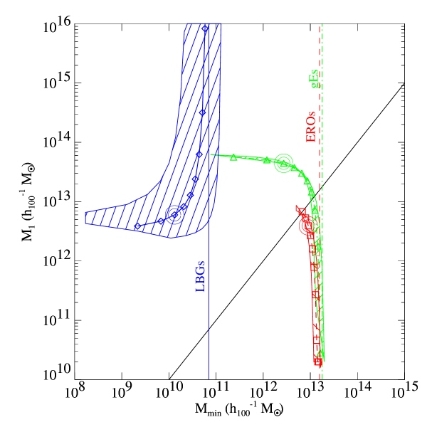
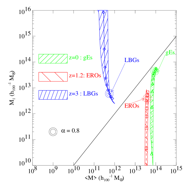
Figure 1: The explicit inversion of the clustering and number density parameters for each galaxy population at its redshift recovers the minimum halo mass and the halo-mass weighted mass, ${\rm M}_{\rm min}$ (left panel) and $\langle{\rm M}\rangle$ (right panel) respectively. This calculation was done for the full range of uncertainties in all observational quantities, as discussed in §2 and summarized in Table 2. Each point indicated corresponds to a different value for the slope of the occupation function, with the range $\alpha=0-1.0$ in intervals of $0.1$. A value of $\alpha\approx 0.8$ (shown by the double-circle points) is shown. The dot-dashed lines with triangles are for $z=0$, $L>L_{*}$ Elliptical galaxies (gEs); the dashed lines with squares are for $z\approx 1.2$ EROs; and the solid lines with diamonds are for $z\approx 3$ LBGs. The labelled vertical lines mark the $\alpha=0$ values for ${\rm M}_{\rm min}$ (see Table 3). Note that the ${\rm M}_{\rm min}$ and $\langle{\rm M}\rangle$ results are relatively insensitive to the occupation function slope $\alpha$ for the strongly-clustered EROs and luminous ellipticals. The solid diagonal lines correspond to ${\rm M}_{\rm min}={\rm M}_{1}$ and $\langle{\rm M}\rangle={\rm M}_{1}$.

In Fig. 1, we show the solutions for the occupation function parameters for the three populations, for different values of the slope $\alpha$. Higher values of ${\rm M}_{\rm min}$ correspond to lower values of $\alpha$. As noted above, the maximum value for ${\rm M}_{\rm min}$ is obtained for the limiting assumption of one object per halo, $\alpha=0$, and is depicted by labelled vertical lines for each case, for the central values of Table 2. The filled areas show the full range of parameter space allowed by the inversion of the chosen values for the number density and correlation length of each population with their stated ($1-\sigma$) uncertainties (Table 2). It should be noted that we have simply used the uncertainties from the literature for a given sample, and have not attempted to include the uncertainty/spread due to sample-to-sample variance or differences in sample selection. These effects will actually lead to a much larger region of allowed parameter space. The minimum mass ${\rm M}_{\rm min}$ is almost independent of $\alpha$ for the strongly clustered local ellipticals and EROs. For the more weakly clustered LBGs, the minimum halo mass is a stronger function of $\alpha$. We also show the average host halo mass $\langle{\rm M}\rangle$ (weighted by galaxy-number), which is even less dependent on $\alpha$ for all cases. From this figure, we see that the clustering and number density of EROs are consistent with their occupying halos of similar masses to those that harbor present-day $L>L_{*}$ ellipticals. In contrast, LBGs must occupy halos that are several orders of magnitude smaller in mass.

The relationship of the values of ${\rm M}_{\rm min}$ and $\langle{\rm M}\rangle$ to those of ${\rm M}_{1}$ is also interesting to consider. Recall that ${\rm M}_{1}$ corresponds to the mass of a halo that harbors on average one galaxy — therefore halos with masses greater than ${\rm M}_{1}$ will tend to contain more than one galaxy. The case ${\rm M}_{1}>\!\!>{\rm M}_{\rm min}$ (above the diagonal lines in Fig. 1) corresponds to a situation where most galaxies are the sole occupants of their dark matter halos. The LBGs fall into this category. Conversely, for ${\rm M}_{1}\lower 2.15277pt\hbox{$\;\buildrel<\over{\sim}\;$}{\rm M}_{\rm min}$, most galaxies have one or more companions within a common dark matter halo. The EROs and gEs are in this category. This is interesting, as it provides indirect evidence for the general concept of hierarchical clustering (i.e., that large structures like groups and clusters are built up over time through merging), and also is even more directly suggestive that EROs, like gEs, are found in group/cluster type environments and may have been influenced by interactions with other galaxies.

Although LBGs are not the main focus of this paper, as they have been the topic of so many analyses of this type, and because our results differ significantly from some of those in the literature, it is worth a brief digression to discuss the reasons for this difference. Some past analyses have used the clustering of LBGs to argue that they are harbored by halos with considerably larger masses of $\simeq 10^{12}{\rm h}_{100}^{-1}{\rm M}_{\odot}$ (e.g. Steidel et al. 1996; Giavalisco et al. 1998). One reason for this is that early results on the observational clustering values based on a few fields yielded considerably larger correlation lengths, $r_{0}=6$ h${}_{100}^{-1}$ Mpc (Adelberger et al. 1998), corresponding to bias values of $b\approx 2.7$ (using our definition of bias). Apparently, the LBGs in these fields showed an unusually strong degree of clustering, and more recent results based on considerably larger areas have yielded lower values; for example, Giavalisco & Dickinson (2001) find $r_{0}=3.2\pm 0.7$ h${}_{100}^{-1}$ Mpc, and Adelberger (2000) finds $r_{0}=3.8\pm 0.3$ h${}_{100}^{-1}$ Mpc (see the broader compilation and discussion in Wechsler et al. 2001). The corresponding values of the linear bias (using our standard definition) are $b\sim 1.4$–1.9. Differing definitions of bias lead to a still broader range of values; for example Adelberger et al. (1998) adopt $b\sim 4$ for the same $\Lambda$CDM model. In addition, most previous analyses of this kind have made the simplifying assumption that each halo above a given mass threshold ${\rm M}_{\rm min}$ contains exactly one galaxy, corresponding to the limiting $\alpha=0$ case discussed above. As one can see from Fig. 2, had we assumed $b\sim 4$ and $\alpha=0$ for LBGs as was done in Adelberger et al. (1998) we would have found ${\rm M}_{\rm min}\sim 10^{12}{\rm h}_{100}^{-1}{\rm M}_{\odot}$, consistent with the value obtained by those authors. Note that our results are also consistent with those of Wechsler et al. (2001), in which a detailed treatment of LBG clustering based on semi-analytic modeling combined with N-body simulations was carried out, and with BWS02, which used an analytic model similar to the one used here. BWS02 obtained further constraints on the slope of the occupation function $0.9\lower 2.15277pt\hbox{$\;\buildrel<\over{\sim}\;$}\alpha\lower 2.15277pt\hbox{$\;\buildrel<\over{\sim}\;$}1.1$ from small scale clustering data.

5 Relating Populations at Different Redshifts

It is always tempting to speculate on the connection of a population observed at high redshift with the more familiar objects in the local Universe. This is a complicated and somewhat ambiguous task in the context of the hierarchical scenario, in which objects do not keep their identity, but are constantly merging and can even change their Hubble type. We cannot try to “follow” the properties of a particular object through time with the simple models presented here, but we can place some constraints on the connections of the three populations we have been discussing with one another, and we can ask specific questions about populations selected in certain ways at different redshifts. This is the topic of this section. We consider two types of models: a classical “galaxy conserving” model, and hierarchical merging models for objects selected with a fixed mass threshold, or with a fixed number density.

The redshift evolution of the comoving correlation scale $r_{0}$ (top); and the linear bias (lower panel), in the galaxy conserving model, for populations as indicated. The filled regions correspond to measured uncertainties, as described in the text and in Fig. 2. The dark solid line in the upper panel shows the correlation scale of the dark matter.

5.1 The galaxy conserving model

First, we consider a very simple null-hypothesis model for describing clustering evolution. If galaxies are assumed to form with some “bias at birth” and then to evolve without merging or changing their luminosity, their relative positions will change solely as dictated by gravity. This is a fluid flow problem, and the behavior of galaxies as tracers of the underlying matter will obey the continuity and Euler equations (Peebles 1980). Fry (1996) worked out this conceptually simple “galaxy conserving” model, wherein the linear bias evolves by

$$b(z)=1+(b_{0}-1)/D(z).$$ (9)

Here, $D$ is the growth factor of the universe for our adopted cosmology, and $b_{0}$ is the “bias at birth” of the population. For $b_{0}$ we can use the bias values at the redshift of observation, and then trace the evolution forward and backward in time again. Implicit in this model is that there is no merging or any loss of identity for any of the galaxy-particles (see also Tegmark & Peebles 1998). In this model, as the universe expands, the bias decreases monotonically and the correlation scale tends towards that of the underlying dark matter (Fry 1996). The results using this model are shown in Fig. 5. If LBGs evolved in this way, they would end up being slightly less clustered than $z=0$ gEs. The extrapolation of EROs’ clustering properties to $z\approx 0$ suggest that they would correspond to a very strongly clustered local population, even more biased than $L>L_{*}$ ellipticals today.

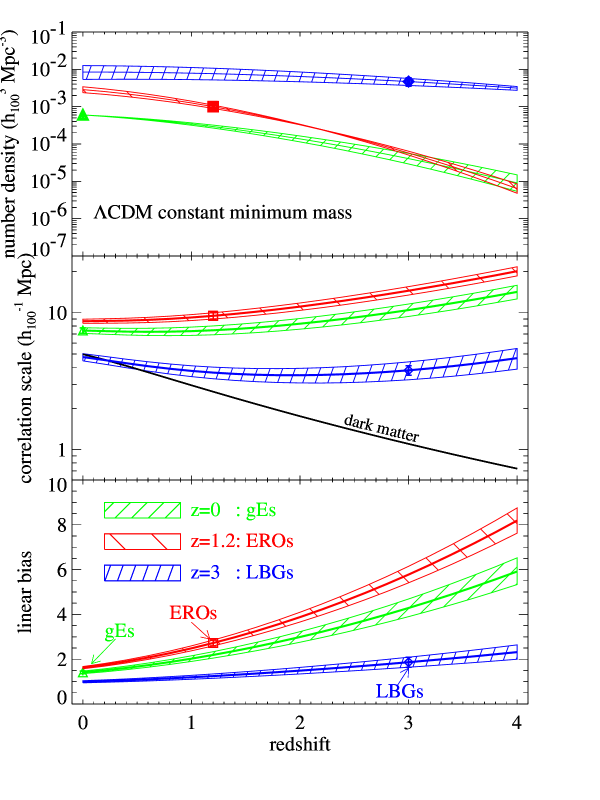
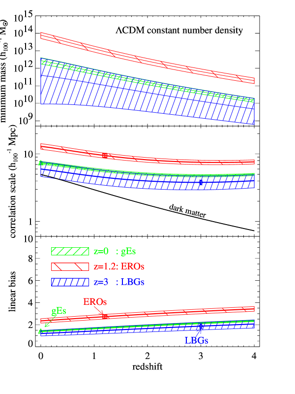
Figure 2: left: In the constant minimum mass model, the redshift evolution of the comoving number density (top panel); the comoving correlation scale $r_{0}$ (middle panel); and the linear bias (lower panel). Each filled region reflects the uncertainties in the values of the occupation function parameters (as shown graphically in the inversion figures of Fig. 1), propagated with redshift by the recipe presented in the text. right: In the constant number density model, the top panel shows the redshift evolution of ${\rm M}_{\rm min}$; the second and third panels are as in the left. The dark matter correlation scale (Eqn. A1) is shown as a solid dark line. These plots are computed for $\alpha=0.8$.

5.2 Hierarchical Merging models

We now use the hierarchical framework presented earlier to produce predictions for the clustering properties of populations selected at different redshifts in two different ways. In the first case, we select objects with a fixed mass threshold (constant minimum mass, “CMM”). Here, we assume that all parameters of the occupation function remain the same, and that halos above a fixed mass threshold (${\rm M}_{\rm min}$) may host galaxies, according to Eqn. 7. We use the occupation function parameters obtained in §4 for each of the three populations, and run these values forward and backward in time to predict clustering properties over a range of cosmological epochs. We also consider the properties of populations selected to have a fixed number density at all redshifts (constant number density, “CND”). Here, we assume that the slope and normalization of the occupation function remain constant over time, but that the minimum mass required to host a galaxy changes, such that the comoving number density of galaxies remains constant. This can be directly connected with observations. As discussed at the beginning of this section, we note again that neither of these models is meant to represent the actual evolution in time of a particular object. Instead, we represent the evolution of statistically defined samples, which may be related to similarly defined observed samples.

Fig. 2 shows how the number density or minimum mass, correlation length, and bias change with time for populations selected in these two ways. We have kept the occupation function slope fixed to $\alpha=0.8$, and we have assumed that the slope of the galaxy correlation function $\gamma_{g}$ is constant with redshift. In the constant mass case, because halos of a fixed mass represent rarer fluctuations in the density field at earlier times, the bias decreases rapidly with time. In the constant number density case, the required ${\rm M}_{\rm min}$ increases with time, so that the bias evolves much less rapidly, but still in the same sense.

In the CMM case, the mass-selected ERO-like population run forward in time are predicted to be slightly more numerous and more clustered than the $z=0$ gEs. This apparently contradictory result is due to the fact that we found that for $\alpha=0.8$, EROs occupy slightly more massive halos than gEs, but ${\rm M}_{1}$ was considerably larger because of the higher number density we adopted for EROs. Concurrent evolution in $\alpha$, ${\rm M}_{1}$, and/or $\gamma_{g}$ could change the details of this prediction; and moreover the value of the number density is quite uncertain. Generally though, this result supports the idea that EROs could be the already mostly assembled progenitors of $z=0$ luminous giant ellipticals. Conversely, the mass-selected LBG-like population is much more numerous and less clustered than either EROs or gEs when run forward in time to $z=0$, because of the relatively low-mass halos they occupy in our model. These results suggest that if LBGs are indeed the progenitors of gEs, they must undergo significant mass-growth through merging between $z=3$ and the present. More speculatively, this perhaps suggests that early type galaxies may have been mostly assembled by $z\sim 1$, but were in much smaller pieces at $z\sim 3$ (or else their progenitors are not associated with the LBGs).

In the CND case, the number-density selected ERO-like objects projected forward in time end up in much more massive halos, and therefore much more clustered, than $z=0$ gEs (but are much less massive and clustered than rich X-ray clusters). The masses and clustering properties of the number-density selected LBG-like objects projected to $z=0$ overlap those of the gEs. This may lead to the same conclusion as the above: that LBGs may evolve into gEs by $z=0$, but must grow in mass considerably.

6 Summary and Conclusions

Extremely Red Objects are an intriguing population which may be the $z\approx 1$ progenitors of giant ellipticals. Recent results from Wide-Field Near-IR selected surveys with multi-band photometry have made it possible to obtain angular clustering and photometric redshift estimates for these objects, allowing the number density and real-space correlation length to be derived from the angular clustering and surface density (Daddi et al. 2001; McCarthy et al. 2001; Firth et al. 2002). These data provide important clues about the nature of EROs by constraining the masses of halos that harbor them in a $\Lambda$CDM hierarchical model of structure formation. We have used an analytic model, combining a simple parameterization of the occupation function of dark matter halos with analytic approximations for halo number density and bias, to constrain the masses of halos harboring EROs. We apply the same approach to $z=0$ ellipticals and $z=3$ LBGs, and using this information, speculate on the connection between these populations and EROs. Our main conclusions may be summarized as follows:

• EROs at $z\sim 1.2$ occupy halos with minimum masses ${\rm M}_{\rm min}\simeq 10^{13}{\rm h}_{100}^{-1}{\rm M}_{\odot}$, with a galaxy-number weighted average halo mass of $\langle{\rm M}\rangle\simeq 5\times 10^{13}{\rm h}_{100}^{-1}{\rm M}_{\odot}$ — in other words, EROs are probably located in rich groups or clusters, at $z\approx 1$. These masses are lower limits for the subset of “old” EROs, if they are associated with larger correlation lengths. These results are rather insensitive to the assumed value of the slope of the occupation function $\alpha$.

• Elliptical galaxies at $z\sim 0$ with $L>L_{*}$ occupy halos with very similar masses to those harboring EROs, lending support to the hypothesis that EROs may be the already almost fully assembled progenitors of present day giant ellipticals.

• Recent results on the measured clustering of Lyman-break galaxies at $z\sim 3$ imply that they occupy much smaller mass halos than EROs or local ellipticals, with ${\rm M}_{\rm min}\approx 10^{10-11}{\rm h}_{100}^{-1}{\rm M}_{\odot}$ and $\langle{\rm M}\rangle\approx 10^{11-12}{\rm h}_{100}^{-1}{\rm M}_{\odot}$. This does not necessarily imply that LBGs are not the progenitors of present-day $L>L_{*}$ ellipticals, only that their halos must experience considerable mass growth via merging if indeed LBGs are to grow into giant ellipticals.

APPENDIX

The correlation function of the dark matter in our chosen cosmology has been computed directly from the GIF/VIRGO N-body $\Lambda$CDM simulation (Jenkins et al. 1998), and is shown in Fig. APPENDIX for several redshifts. Approximating the correlation function on linear scales with a power-law, we parametrize the comoving correlation length scale $r_{0}$ and the correlation function slope $\gamma$ as a function of redshift in a convenient analytic form:

$$\log_{10}({\rm h}_{100}^{-1}\,r_{0_{\rm DM}}) = \log_{10}(5.00)-0.00142-$$ (A1)

$$0.419\,\log_{10}(1+z)-$$

$$1.11\,\log_{10}(1+z)^{2},$$

$$\gamma_{0_{\rm DM}} = -1.74+0.169\,z.$$ (A2)

left: The spatial correlation function, $\xi_{\rm DM}(r)$, of dark matter based on the GIF/VIRGO $\Lambda$CDM simulation, computed directly at redshifts 0.0, 0.5, 1.0, 2.0, and 3.0. The correlation strength decreases with increasing redshift, as shown in the legend. Linear regressions are computed for $r_{\rm 0,DM}>2.5$ h${}_{100}^{-1}$ Mpc (to the right of the dotted line), and are shown as solid lines over the measurements. From these fits, relevant for the $r=8$ h${}_{100}^{-1}$ Mpc scale considered in this paper, the correlation length ($r_{\rm 0,DM}$) and power ($\gamma_{\rm DM}$) are computed. Best-fitting polynomial fits are given in Eqns. A1 and A2, and shown with the data in the right panel.

Table 1: Dark Matter Clustering Properties

Parameter	$z=0$	$z=1.2$	$z=3$
$\xi_{8,{\rm DM}}$	$\phantom{-}0.439$	$\phantom{-}0.173$	$\phantom{-}0.087$
$r_{0,{\rm DM}}\,({\rm h}_{100}^{-1}\,{\rm Mpc})$	$\phantom{-}4.981$	$\phantom{-}2.513$	$\phantom{-}1.101$
$\gamma_{\rm DM}$	$-1.736$	$-1.517$	$-1.229$

Table 2: Observational Values used for Analysis

Parameter	gEs	EROs	LBGs
	$z=0$	$z=1.2$	$z=3.0$
$n$ (h${}_{100}^{3}$ Mpc-3)	$6.0$ $\cdot{}$ 10-4	$\cdot{}$ 10-3($1.0\pm 0.1$) $\cdot{}$ 10-3	$\cdot{}$ 10-3($4.7\pm 1.0$) $\cdot{}$ 10-3
$r_{0,{\rm g}}\,\,({\rm h}_{100}^{-1}\,{\rm Mpc})$	$7.42\pm 0.33$	$\phantom{0.5}9.5\pm 0.5\phantom{9.5}$	$3.8\pm 0.3$
$\gamma_{\rm g}$	$-1.76\pm 0.04\phantom{-}$	$-1.8\phantom{\pm-1.8}$	$-1.60\pm 0.15\phantom{-}$
$\xi_{8,{g}}$	$0.88\pm 0.07$	$1.36\pm 0.13$	$0.30\pm 0.08$
b	$1.41\pm 0.06$	$2.7\pm 0.1$	$1.9\pm 0.2$

Table 3: Characteristic Population Masses

		$\alpha=0$		$\alpha=0.8$
Population	$z$	${\rm M}_{\rm min}$ (h${}_{100}^{-1}$ M⊙)		${\rm M}_{\rm min}$ (h${}_{100}^{-1}$ M⊙)	$M_{1}$ (h${}_{100}^{-1}$ M⊙)	$\langle{\rm M}\rangle$ (h${}_{100}^{-1}$ M⊙)
gEs	0.0	1.7 $\cdot{}$ $10^{13}$		2.7 $\cdot{}10^{12}$	4.4 $\cdot{}10^{13}$	8.9 $\cdot{}10^{13}$
EROs	1.2	1.6 $\cdot{}$ $10^{13}$		9.1 $\cdot{}10^{12}$	3.9 $\cdot{}10^{12}$	3.8 $\cdot{}10^{13}$
LBGs	3.0	7.0 $\cdot{}$ $10^{10}$		1.3 $\cdot{}10^{10}$	6.0 $\cdot{}10^{12}$	5.5 $\cdot{}10^{11}$

References

- Adelberger (2000) Adelberger, K. 2000, in ASP Conf. Ser. 200: Clustering at High Redshift, 13
- Adelberger et al. (1998) Adelberger, K. L., Steidel, C. C., Giavalisco, M., Dickinson, M., Pettini, M., & Kellogg, M. 1998, ApJ, 505, 18, (A98)
- Barger et al. (1999) Barger, A. J., Cowie, L. L., Trentham, N., Fulton, E., Hu, E. M., Songaila, A., & Hall, D. 1999, AJ, 117, 102
- Benson et al. (2000) Benson, A. J., Cole, S., Frenk, C. S., Baugh, C. M., & Lacey, C. G. 2000, MNRAS, 311, 793
- Benson et al. (2001) Benson, A. J., Pearce, F. R., Frenk, C. S., Baugh, C. M., & Jenkins, A. 2001, MNRAS, 320, 261
- Berlind & Weinberg (2001) Berlind, A. A. & Weinberg, D. H. 2001, ApJ, submitted (astro-ph/0109001)
- Brown et al. (2000) Brown, M. J. I., Webster, R. L., & Boyle, B. J. 2000, MNRAS, 317, 782
- Bullock et al. (2001) Bullock, J. S., Wechsler, R. H., & Somerville, R. S. 2001, MNRAS, 329, 246 (BWS02)
- Cabanac et al. (2000) Cabanac, R. A., de Lapparent, V., & Hickson, P. 2000, A&A, 364, 349
- Chen et al. (2002) Chen, H., et al. 2002, ApJ, 570, 54
- Cimatti et al. (2002) Cimatti, A., et al. 2002, A&A, 381, L68
- Cole et al. (2000) Cole, S., Lacey, C. G., Baugh, C. M., & Frenk, C. S. 2000, MNRAS, 319, 168
- Collins et al. (2000) Collins, C. A., et al. 2000, MNRAS, 319, 939
- Cowie et al. (1994) Cowie, L. L., Gardner, J. P., Hu, E. M., Songaila, A., Hodapp, K.-W., & Wainscoat, R. J. 1994, ApJ, 434, 114
- Daddi et al. (2001) Daddi, E., Broadhurst, T., Zamorani, G., Cimatti, A., Röttgering, H., & Renzini, A. 2001, A&A, 376, 825
- Daddi et al. (2002) Daddi, E., et al. 2002, A&A, 384, L1
- Daddi et al. (2000) Daddi, E., Cimatti, A., Pozzetti, L., Hoekstra, H., Röttgering, H. J. A., Renzini, A., Zamorani, G., & Mannucci, F. 2000, A&A, 361, 535
- Dunlop et al. (1996) Dunlop, J., Peacock, J., Spinrad, H., Dey, A., Jimenez, R., Stern, D., & Windhorst, R. 1996, Nature, 381, 581
- Eggen et al. (1962) Eggen, O. J., Lynden-Bell, D., & Sandage, A. R. 1962, ApJ, 136, 748
- Elston et al. (1988) Elston, R., Rieke, G. H., & Rieke, M. J. 1988, ApJ, 331, L77
- Elston et al. (1989) Elston, R., Rieke, M. J., & Rieke, G. H. 1989, ApJ, 341, 80
- Firth et al. (2002) Firth, A. E., et al. 2002, MNRAS, 332, 617
- Fry (1996) Fry, J. N. 1996, ApJ, 461, L65
- Giavalisco & Dickinson (2001) Giavalisco, M. & Dickinson, M. E. 2001, ApJ, 550, 177
- Giavalisco et al. (1998) Giavalisco, M., Steidel, C. C., Adelberger, K. L., Dickinson, M. E., Pettini, M., & Kellogg, M. 1998, ApJ, 503, 543
- Graham & Dey (1996) Graham, J. R. & Dey, A. 1996, ApJ, 471, 720
- Hermit et al. (1996) Hermit, S., Santiago, B. X., Lahav, O., Strauss, M. A., Davis, M., Dressler, A., & Huchra, J. P. 1996, MNRAS, 283, 709
- Hu & Ridgway (1994) Hu, E. M. & Ridgway, S. E. 1994, AJ, 107, 1303
- Jenkins et al. (1998) Jenkins, A., et al. 1998, ApJ, 499, 20
- Jenkins et al. (2001) Jenkins, A., Frenk, C. S., White, S. D. M., Colberg, J. M., Cole, S., Evrard, A. E., Couchman, H. M. P., & Yoshida, N. 2001, MNRAS, 321, 372
- Jing, Mo, & Börner (1998) Jing, Y. P., Mo, H. J., & Börner, G. 1998, ApJ, 494, 1
- Katz et al. (1999) Katz, N., Hernquist, L., & Weinberg, D. H. 1999, ApJ, 523, 463
- Kauffmann et al. (1999) Kauffmann, G., Colberg, J. M., Diaferio, A., & White, S. D. M. 1999, MNRAS, 307, 529
- Loveday et al. (1995) Loveday, J., Maddox, S. J., Efstathiou, G., & Peterson, B. A. 1995, ApJ, 442, 457
- Marinoni & Hudson (2002) Marinoni, C. & Hudson, M. J. 2002, ApJ, 569, 101
- Martini (2001) Martini, P. 2001, AJ, 121, 2301
- McCarthy et al. (2001) McCarthy, P. J., et al. 2001, ApJ, 560, L131
- McCarthy et al. (1992) McCarthy, P. J., Persson, S. E., & West, S. C. 1992, ApJ, 386, 52
- Mo & White (1996) Mo, H. J. & White, S. D. M. 1996, MNRAS, 282, 347
- Moriondo et al. (2000) Moriondo, G., Cimatti, A., & Daddi, E. 2000, A&A, 364, 26
- Moustakas et al. (1997) Moustakas, L. A., Davis, M., Graham, J. R., Silk, J., Peterson, B. A., & Yoshii, Y. 1997, ApJ, 475, 445
- Norberg et al. (2002) Norberg, P., et al. 2002, MNRAS, submitted, astro-ph/0112043
- Olding et al. (2002) Olding, E. J., Dalton, G. B., Moustakas, L. A., Booth, J., & Wegner, G. A. 2002, MNRAS, submitted
- Peacock & Smith (2000) Peacock, J. A. & Smith, R. E. 2000, MNRAS, 318, 1144
- Peebles (1980) Peebles, P. 1980, The Large-Scale Structure of the Universe (Princeton University Press)
- Pozzetti & Mannucci (2000) Pozzetti, L. & Mannucci, F. 2000, MNRAS, 317, L17
- Press & Schechter (1974) Press, W. H. & Schechter, P. 1974, ApJ, 187, 425
- Scoccimarro et al. (2001) Scoccimarro, R., Sheth, R. K., Hui, L., & Jain, B. 2001, ApJ, 546, 20
- Seljak (2001) Seljak, U. 2001, MNRAS, 325, 1359
- Sheth & Tormen (1999) Sheth, R. K. & Tormen, G. 1999, MNRAS, 308, 119
- Smail et al. (1999) Smail, I., Ivison, R. J., Kneib, J.-P., Cowie, L. L., Blain, A. W., Barger, A. J., Owen, F. N., & Morrison, G. 1999, MNRAS, 308, 1061
- Somerville et al. (2001a) Somerville, R. S., Lemson, G., Sigad, Y., Dekel, A., Kauffmann, G., & White, S. D. M. 2001a, MNRAS, 320, 289
- Somerville & Primack (1999) Somerville, R. S. & Primack, J. R. 1999, MNRAS, 310, 1087, (SP)
- Somerville et al. (2001b) Somerville, R. S., Primack, J. R., & Faber, S. M. 2001b, MNRAS, 320, 504
- Spinrad et al. (1997) Spinrad, H., Dey, A., Stern, D., Dunlop, J., Peacock, J., Jimenez, R., & Windhorst, R. 1997, ApJ, 484, 581
- Steidel et al. (1996) Steidel, C., Giavalisco, M., Pettini, M., Dickinson, M., & Adelberger, K. 1996, ApJ, 462, L17
- Steidel et al. (1999) Steidel, C. C., Adelberger, K. L., Giavalisco, M., Dickinson, M., & Pettini, M. 1999, ApJ, 519, 1
- Tegmark & Peebles (1998) Tegmark, M. & Peebles, P. J. E. 1998, ApJ, 500, L79
- Thompson et al. (1999) Thompson, D., et al. 1999, ApJ, 523, 100
- Wechsler et al. (2001) Wechsler, R. H., Somerville, R. S., Bullock, J. S., Kolatt, T. S., Primack, J. R., Blumenthal, G. R., & Dekel, A. 2001, ApJ, 554, 85
- White et al. (2001) White, M., Hernquist, L., & Springel, V. 2001, ApJ, 550, L129
- Willmer et al. (1998) Willmer, C. N. A., da Costa, L. N., & Pellegrini, P. S. 1998, AJ, 115, 869
- Zehavi et al. (2002) Zehavi, I., et al. 2002, ApJ, submitted, astro-ph/0106476