High-resolution H i Mapping of NGC 4038/9 (“The Antennae”) and its Tidal Dwarf Galaxy Candidates

Abstract

We present new VLA C+D-array H i observations and optical and NIR imaging of the well known interacting system NGC 4038/9, “The Antennae”. At low spatial resolution ($\sim 40^{\prime\prime}$), the radio data reach a limiting column density of $\sim 10^{19}$ cm${}^{-2}\,(2.5\sigma)$, providing significantly deeper mapping of the tidal features than afforded by earlier H i maps. At relatively high spatial resolution ($\sim 10^{\prime\prime}$), the radio data reveal a wealth of gaseous sub-structure both within the main bodies of the galaxies and along the tidal tails. In agreement with previous H i studies, we find that the northern tail has H i along its outer length, but none along its base. We suggest that the H i at the base of this tail has been ionized by massive stars in the disk of NGC 4038. The gas in the southern tail has a bifurcated structure, with one filament lying along the optical tail and another running parallel to it but with no optical counterpart. The two filaments join just before the location of several star forming regions near the end of the tail. The H i velocity field at the end of the tail is dominated by strong velocity gradients which suggest that at this location the tail is bending away from us. We delineate and examine two regions within the tail previously identified as possible sites of a so-called “tidal dwarf galaxy” condensing out of the expanding tidal material. The tail velocity gradients mask any clear kinematic signature of a self-gravitating condensation in this region. A dynamical analysis suggest that there is not enough mass in gas alone for either of these regions to be self-gravitating. Conversely, if they are bound they require a significant contribution to their dynamical mass from evolved stars or dark matter. Even if there are no distinct dynamical tidal entities, it is clear that there is a unique concentration of gas, stars and star forming regions within the southern tail: the H i channel maps show clear evidence for a significant condensation near the tail star forming regions, with the single-channel H i column densities higher than anywhere else in the system, including within the main disks. Finally, the data reveal H i emission associated with the edge-on “superthin” Scd galaxy ESO 572–G045 that lies just beyond the southern tidal tail of The Antennae, showing it to be a companion system.

1. Introduction

NGC 4038/9 (= Arp 244), aptly nicknamed “The Antennae”, is one of the best-studied examples a galactic collision. The long tails which distinguish this system are emblematic of violent tidal interactions between disk galaxies of similar mass (Toomre & Toomre 1972, Schweizer 1978). Tidal tails originate from the outer regions of galactic disks and are often rich in neutral atomic hydrogen. These features develop kinematically and their velocity fields bear the imprint of the encounter process, so they provide crucial information for dynamical modeling of interacting galaxies. We therefore targeted NGC 4038/9 for high-spatial and velocity resolution H i observations (full-width at half maximum, FWHM, as fine as $\sim 10^{\prime\prime};\Delta v\sim$ 5 km s^-1) in order to obtain the data needed to constrain future numerical simulations of this system.

NGC 4038/9 was the first major merger to be mapped in the 21-cm line of neutral hydrogen. The presence of significant quantities of neutral hydrogen within both the main bodies and the tails of NGC 4038/9 was established from single-dish measurements (Peterson & Shostak 1974, Huchtmeier & Bohnenstengel 1975). Subsequently, NGC 4038/9 has been the subject of H i synthesis mapping observations using the Westerbork Synthesis Radio Telescope (WSRT; van der Hulst 1979a), the Very Large Array (VLA; Mahoney, Burke & van der Hulst 1987) and the Australian Telescope Compact Array (ATCA; Gordon, Koribalski & Jones 2001). The observations reported in this paper provide a more detailed mapping of the tidal features than afforded by previously published H i maps, representing an improvement in spatial and velocity resolution by over a factor of two.

Other spectral line studies have mapped the kinematics of NGC 4038/9 using CO spectral lines (Stanford et al. 1990, Wilson et al. 2000, Gao et al.  2001, Zhu 2001) and optical emission lines (Burbidge & Burbidge 1966, Ruben, Ford & D’Odorico 1970, Amram et al. 1992). However, the molecular and ionized gas is confined to the inner disk regions, and their kinematics do not constrain the encounter geometry as well as that of the tidal tails.

At a heliocentric velocity of 1630 km s^-1 (corresponding to a velocity relative to the local group of 1440 km s^-1), The Antennae is one of the nearest on-going major mergers. To be consistent with the majority of the recent work on NGC 4038/9, we derive physical quantities by adopting a Hubble Constant of 75 km s^-1 Mpc^-1, yielding a distance of 19.2 Mpc. However, a recent analysis of $HST$ $VI$ photometry of individual stars within the southern tidal tail of NGC 4038/9 by Saviane, Rich & Hibbard (2001) suggests a much smaller distance of 13.8$\pm$0.5 Mpc. This distance is derived by identifying luminous red stars within the tail with the red giant branch of an old, metal poor population. There are some caveats to this derivation, for which we refer the reader to Saviane et al., so for the purposes of the present work, we will use the more commonly accepted value of 19.2 Mpc.

At this distance, the tidal tails of NGC 4038/9 extend some 65 kpc in radius and measure $\sim 110$ kpc from end to end. The bodies of the galaxies are sites of extensive star formation, producing an IR luminosity of $\log(L_{\rm IR})=10.76$ and an IR to blue luminosity ratio of $L_{\rm IR}/L_{\rm B}\simeq 6$. Long-wavelength studies from the NIR to Radio suggest that this luminosity is powered by an active system-wide starburst, with no indication of a significant contribution by an AGN (Hummel & van der Hulst 1986, Vigroux et al.  1996, Fischer et al.  1996, Kunze et al.  1996, Mirabel et al.  1998, Nikola, T. et al. 1998, Laurent et al. 2000, Haas et al. 2000, Xu et al. 2000, Neff & Ulvestad 2000, Mengel et al. 2001). While the IR luminosity is an order of magnitude lower than the most active star forming mergers (the so-called Ultraluminous Infrared Galaxies), it is still a factor of $\sim$5 higher than non-interacting galaxy pairs (e.g. Kennicutt et al. 1987, Bushouse 1987, Bushouse, Lamb & Werner 1988), with an inferred star formation rate (SFR) of $\sim 20\,M_{\odot}\,{\rm yr}^{-1}$ (Evans, Harper & Helou 1997; Zhang, Fall & Whitmore 2001).

NGC 4038/9 is the nearest system with an identified dwarf-galaxy sized concentration of gas, light and young stars embedded within a luminous tidal tail (Schweizer 1978, hereafter S78; Mirabel, Dottori, & Lutz 1992, hereafter MDL92). Such concentrations have been known for quite some time (e.g. Zwicky 1956), but have only recently received detailed attention. Several numerical studies lend support to the hypothesis that such systems are self-gravitating and may evolve into independent dwarf galaxies (Barnes & Hernquist 1992, Elmegreen, Kaufmann & Thomasson 1993), but the supporting observational evidence is primarily circumstantial. These observations show that the optical condensations within tidal tails contain many young stars (S78, MDL92, Hunsberger, Charlton, & Zaritsky 1998, Weilbacher et al. 2000, Iglesias-Páramo & Vílchez 2001, Saviane, Rich & Hibbard 2001) and have global properties, such as size, luminosity, H i mass, H i velocity dispersion, and CO content, in common with dwarf Irregular galaxies (Mirabel et al. 1992; Hibbard et al. 1994; Smith & Higdon 1994; Duc & Mirabel 1994, Duc et al. 1997, 2000; Smith & Struck 2001; Braine et al. 2000, 2001). Recently, some tidal dwarfs have even been found to harbor “Super Star Clusters” (Knierman et al. 2001). For these reasons, such concentrations are often referred to as “Tidal Dwarf Galaxies” (hereafter TDGs). However, strong kinematic evidence that these concentrations are indeed self-gravitating is lacking, and their evolution into dwarfs is therefore still in question (see Hibbard, Barnes, & van der Hulst 2001, hereafter Paper II, for more details). Another objective of the present observations is therefore to search for the kinematic signature of a self-gravitating mass in the vicinity of the putative TDG.

The paper is organized in the following manner. In §2 we present details on the observations and data reduction procedures. In §3 we describe in turn the morphology and kinematics of the tidal tails, sub-structure within the tails, the region in the vicinity of the TDG, the inner disks, and the companion galaxy. In §4 we try to explain various aspects of the H i tidal morphology, and look for evidence for a kinematically distinct entity at the end of the southern tail. Our conclusions are presented in §5.

2. Observations

2.1. VLA H i  Observations

The Antennae was observed in two separate array configuration of the VLA radio interferometer: the most compact configuration (1 km D-array) in June of 1996, and the hybrid CnB-array in June of 1997. For the hybrid array, the antennae along the E and W arms of the array are at the standard C-array (3 km) stations while those of the N arm are at the more extended B-array (9 km) stations. This compensates for the foreshortening of baselines to the north arm antennae that occurs for sources at low declination. The short baselines of the D-array provide the highest sensitivity to extended gas, while the longer baselines of the CnB-array allow resolutions as fine as $\sim 10^{\prime\prime}$. NGC 4038/9 was observed for a total of 3.5 hours in the D-array and 8 hours in the CnB-array. The details of these observations are tabulated in Table 1.

We observed using the 21-cm spectral line mode with the system tuned to a central frequency corresponding to a heliocentric velocity of 1630 km s^-1, the central velocity of the existing H i  synthesis observations (Mahoney et al.  1987). Since the atomic gas within tidal tails typically has narrow linewidths ($\sigma_{v}\sim$ 5—10 km s^-1; Hibbard et al.  1994, Hibbard & van Gorkom 1996), the correlator mode was chosen to give the smallest channel spacing while still covering the velocity spread of existing H i  observations (1360–1860 km s^-1; van der Hulst 1979a, Mahoney et al.  1987). New broader-bandwidth H i (Gordon et al. 2001) and CO (Gao et al. 2001) observations reveal that there is both atomic and molecular gas over the velocity range from 1340–1945 km s^-1. We discuss the implications of this result below.

Using on-line Hanning smoothing, the chosen set-up provides 127 independent velocity channels over the 3.125 MHz bandwidth, resulting in a channel spacing of 5.21 km s^-1. The pointing center was chosen to place the ends of the optical tails at equal distances from the phase center. This position is $2\farcm 5$ south of the main bodies, and places the ends of the optical tails at a radius of $\sim 10^{\prime}$, which is approximately the 75% sensitivity point of the primary beam (see Figure 1).

The data were calibrated, mapped, and “Cleaned” using standard techniques and procedures in the Astronomical Image Processing System (AIPS) (see e.g. Rupen 1999). The data from the separate arrays were calibrated and bandpass corrected independently, after which they were combined in the UV plane to produce the C+D dataset. This latter dataset is used exclusively throughout this paper. The final calibration of this dataset was achieved by three iterations of a phase-only self-calibration. The resulting continuum map is very similar to others that have appeared in the literature (e.g. Hummel & van der Hulst 1986; Neff & Ulvestad 2000, Gordon et al. 2001), and is not shown here.

The continuum was subtracted from the velocity cube by fitting a first-order polynomial to the visibilities from the line free channels on either end of the bandpass. This is done in an iterative manner in order to determine which channels are free of line emission. The resulting fit was made using channels 11–20 and 104–111 of the 127 channel cube, corresponding to the velocities 1859–1911 km s^-1 and 1386–1423 km s^-1. As mentioned above, cold gas has been found within both of these velocity ranges by Gordon et al. (2001) and Gao et al. (2001). The gas at these velocities is of low surface brightness and totally confined to either the disk of NGC 4039 or the disk overlap region. Therefore, using this continuum range will not affect any of the measured properties of the tidal tails, which is our primary interest in this paper. However, the H i flux we measure for the central region will underestimate the true flux, and the kinematics of this region will not be accurately mapped (although the fact that the line kinematics are weighted by intensity will somewhat mitigate the effects of the missing velocity information).

The continuum subtracted data were mapped using several values of the Robust weighting parameter, $R$ (Briggs 1995). This parameter can be varied to emphasize either the outer ($R<0$) or the inner ($R>0$) regions of the UV plane (i.e., either small or large spatial scales). In practical terms, a lower $R$ gives a finer spatial resolution at the expense of surface brightness sensitivity, while a larger $R$ gives a higher surface brightness sensitivity at a slightly coarser spatial resolution. A high resolution data cube was made with $R=-1$, providing a surface brightness rms sensitivity of 1.3 mJy beam^-1 at a resolution of $\theta_{FWHM}=11.4^{\prime\prime}\times 7.4^{\prime\prime}$. This corresponds to a single channel column density limit (2.5$\sigma$ per channel) of 2.2$\times 10^{20}\,{\rm cm}^{-2}$ averaged over the beam width of 1.1$\times$0.7 kpc². A more sensitive intermediate resolution data cube, made with $R=+1$, provides a resolution of $21^{\prime\prime}\times 15^{\prime\prime}$ (1.9$\times$1.4 kpc²) and a column density limit of 4$\times 10^{19}\,{\rm cm}^{-2}$. To further increase sensitivity to extended low column density gas, a low resolution data cube was made by convolving the $R=+1$ data cube to a resolution of $40^{\prime\prime}$ (3.7 kpc), reaching a detection limit of 1.2$\times 10^{19}\,{\rm cm}^{-2}$. These data will be referred to in the following as the high, intermediate, and low resolution data, respectively. These parameters are summarized in Table 1. The resulting per channel noise is close to theoretical once the higher system temperature due to the low declination of the source is taken into consideration.

Visualization of the resulting data cubes and inter-comparison with the optical and NIR data was greatly facilitated by using the Karma visualization package (Gooch 1995). Besides allowing multiple images to be interactively compared, this package also allows a full 3-dimensional rendering of datacubes, which is a particularly powerful tool for disturbed systems.

After a careful viewing, the data cubes were integrated over the velocity axis to produce the moment maps. In order to suppress the effects of noise, only data above a fixed threshold are used in the moment summation (the “cutoff technique” described by Bosma, 1981) using the AIPS task MOMNT. This task applies a user specified threshold to a version of the data cube smoothed in both space and velocity. If a pixel in the smoothed data cube passes the threshold, the corresponding pixel in the un-smoothed data is included in the moment analysis. This procedure favors low level emission that is extended in velocity and/or space over emission which is isolated. The output from this analysis is an integrated intensity map (zeroth moment), an intensity-weighted velocity map (first moment), and an intensity-weighted velocity dispersion map (second moment). It should be noted that the first and second moment maps give an accurate representation of the mean H i  velocity and line-of-sight velocity dispersion at a location only if the line profiles are single-peaked. The final zeroth moment maps were corrected for the primary beam attenuation before measuring H i  fluxes.

We measure H i fluxes from an integrated intensity map constructed to match the new ATCA H i observations of Gordon et al. (2001), since those authors were able to do a proper line-free continuum subtraction. For the moment analysis, this involved applying a threshold of 2.1 mJy beam^-1 to the data after smoothing with a 3$\times$3 pixel boxcar spatial filter and a five-channel Hanning filter. Our resulting flux measurements are given in Table 3. The errors attached to the flux measurements have been determined from the single channel noise by properly taking into account the number of independent channels and beams over which the flux was integrated. It should be noted that the error calculation does not include systematic errors, such as those introduced by poor continuum subtraction or incomplete cleaning.

2.2. Optical and NIR Observations

The supporting optical observations were obtained during two nights of broad-band $BVR$ imaging on the CTIO 0.9m with the Tek512 CCD in April of 1991 and one night of near-Infrared (NIR) $K^{\prime}$-band imaging on the UH $88^{\prime\prime}$ with the QUIRC detector in January of 1995. The details of these runs are given in Table 2. For the optical run the conditions were photometric and the seeing was $\sim 1^{\prime\prime}$. The f/13.5 re-imaging optics were used, giving a plate scale of $0.44^{\prime\prime}$ pixel^-1 and a field of view of 3.8^′. The data were calibrated via observations of standards in the Graham E-regions (Graham 1982) observed on the same nights, with zeropoint errors (1$\sigma$) of 0.04^m in $B$ and 0.02^m in both $V$ and $R$. For the NIR run, the data were obtained through a $K^{\prime}$ filter ($\lambda=2.11\mu$m, $\Delta\lambda=0.35\mu$m; Wainscoat & Cowie 1992; hereafter referred to simply as $K$). The f/10 re-imaging optics were used, resulting in a plate scale of $0.187^{\prime\prime}$ pixel^-1 and a field of view of 3$\farcm$2. The seeing was $\sim 1^{\prime\prime}$. These observations consist of three 120 sec target-sky pairs, with the CCD dithered by 1$\farcm$5 between on-source positions. The NIR data are uncalibrated.

The combined images were transformed to the World Coordinate System (and thereby to the same reference frame as the radio images) by registering to an image of the same area extracted from the Digitized Sky Survey (DSS). The registration was accomplished by referencing the location of $\sim$ 20 stars in common on both images using the koords program in the Karma package (Gooch 1995) to perform a non-linear least squares fit for the transformation equations. The plate solution so found is accurate to a fraction of a pixel, and the overall registration should be as good as that of the southern portion of the Guide Star Catalog, which is estimated to be $0\farcs 7$ (Taff et al. 1990).

Deep optical images were constructed by applying a 9$\times$9 pixel boxcar median to the pixels with the lowest light levels, achieving limiting surface brightnesses of $\mu_{B}$=27.0 mag arcsec^-2  and $\mu_{R}$=26.5 mag arcsec^-2. Color maps in $B-R$ and $B-K$ were made after convolving the images to a common resolution, and using only pixels with a signal-to-noise greater than five in both bands. These maps will be shown here, but a full color analysis is deferred to a later paper (Evans et al., in prep.). Finally, a smoothed $B$-band image was made by replacing stars with background values and convolving to the resolution of the intermediate resolution H i  data. This image is used to evaluate the H i  mass to blue light ratio ($M_{HI}/L_{B}$) of various regions.

3. Results

The large scale distribution of the H i  is shown in Figure 1, where the left panel shows the low resolution H i  contoured upon the DSS image, while the right panel shows the intermediate resolution H i in greyscales with contours from the smoothed $B$-band superimposed. Our new observations delineate the distribution of tidal H i much more clearly than earlier H i observations, showing that the gas in the northern tail extends further than previously known, and revealing a small H i-rich disk companion to The Antennae lying just beyond the southern tail. These results are confirmed by the ATCA observations by Gordon et al. (2001). Using the NASA Extragalactic Database (NED), this latter object is identified with the galaxy ESO 572–G045. We break the H i emission into four separate components: the southern tail, the northern tail, the inner disks, and the new dwarf companion ESO 572–G045. The H i properties of each of these components are listed in Table 3.

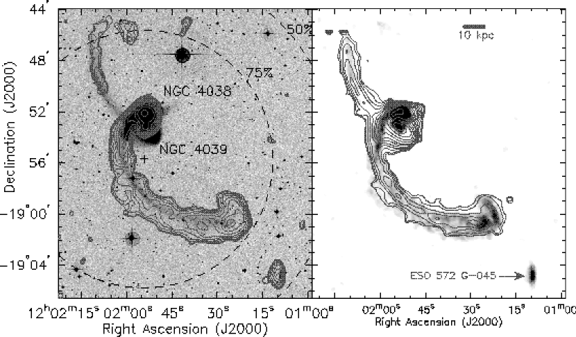
Figure 1.— Left: Integrated H i  emission contoured upon on a greyscale representation of the DSS image of “The Antennae”. The cross marks the phase center of the VLA observations, while the dashed circles represent the 75% and 50% response points of the VLA primary beam. The two main disks, NGC 4038 and NGC 4039, are labeled, as is the companion galaxy ESO 572 G–045. The contours are from the low resolution (40^′′) datacube, and are are drawn at flux levels of (5, 10, 20, …) $\times$14.49 mJy beam^-1 km s^-1, with the lowest contour corresponding to an H i column density of 5$\times 10^{19}\,{\rm cm}^{-2}$. Right: Greyscale representation of the intermediate resolution H i ($20.7^{\prime\prime}\times 15.4^{\prime\prime}$), with contours from the $B$-band image, after star subtraction and convolving to a resolution of $25^{\prime\prime}$. Optical contours are drawn from 27 mag arcsec^-2 to 20.5 mag arcsec^-2 in intervals of 0.5 mag arcsec^-2. The box-like optical contours to the northwest of the disk indicate the extent of the CCD frame in this direction. The scale bar indicates a length of 10 kpc for a distance of 19.2 Mpc.

The large scale distribution and kinematics of the H i  derived from the intermediate resolution data are shown in Figure 2. The upper left panel shows a false color representation of the data, with the H i  shown in blue and starlight in green and white. The upper right panel of Fig. 2 shows the $B-R$ color map with $B$-band surface brightness contours superimposed. The lower left panel shows a color representation of the intensity weighted H i velocity field with iso-velocity contours superimposed. Finally, the lower right panel shows a color representation of the H i  velocity dispersion, again with H i  column density contours superimposed.

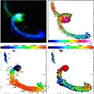
Figure 2.— Large scale distribution of the H i  and optical light in NGC 4038/9. The upper left panel shows a false color representation of the intermediate resolution H i data (blue), and the CTIO $B+V+R$ combined image in green and white. The upper right panel of shows the $B-R$ color map, where colors have been determined for pixels with a S/N $>$ 5 ($\mu_{B}<$ 26.4 mag arcsec^-2). Blue colors correspond to $[B-R<0.5]$, light blue/cyan to $[0.5<B-R<0.7]$, green to $[0.7<B-R<0.9]$, yellow/orange to $[0.9<B-R<1.1]$, red to $[1.1<B-R<1.3]$, magenta to $[1.3<B-R<1.5]$, and white to $[B-R>1.5]$. Surface brightness contours from the star-subtracted $B$-band image convolved to 25^′′ resolution are drawn at intervals of (26.5, 26, 25.5, …, 20.5) mag arcsec^-2. The lower left panel shows the intensity weighted H i velocities (green indicates velocities close to systemic, and red and blue indicate redshifted and blueshifted velocities, respectively) with isovelocity contours drawn at 10 km s^-1 intervals. The lower right panel maps the H i velocity dispersion with the intermediate H i column density contours superimposed. In this panel blue/cyan corresponds to [$\sigma_{HI}<5.0$ km s^-1], green to [$5.0<\sigma_{HI}<9.0$ km s^-1], yellow/orange to [$9.0<\sigma_{HI}<13.0$ km s^-1], and red to [$\sigma_{HI}>13.0$ km s^-1]. H i column densities are drawn at levels of (1, 2, 4, 8, …) $\times$28.88 mJy beam^-1 km s^-1, where the lowest contour corresponds to 1$\times 10^{20}\,{\rm cm}^{-2}$.

As revealed by the WSRT observations of van der Hulst (1979a), the majority of the H i is associated with NGC 4038 and the southern tail, with much less gas directly associated with NGC 4039 and the northern tail. We detect tidal H i emission over a velocity range of 1420 – 1850 km s^-1, similar to that found in the synthesis observations of Mahoney et al. (1987), but less than found in the broader bandwidth observations of Gordon et al. (2001). We measure a total H i flux of at least 54.5$\pm$0.5 Jy km s^-1 for NGC 4038/9, corresponding to a H i mass of $>$4.7$\times 10^{9}M_{\odot}$ (Table 3). This is not very different from the total flux measurement of 57.1 Jy km s^-1 measured at the ATCA by Gordon et al. (2001). However, when we divide the emission among the different components we do find differences. We measure a total flux of 49.7 Jy km s^-1 associated with the main disks and southern tail, compared to the 55.1 Jy km s^-1 measured by Gordon et al.. Examining the channel maps of Gordon et al., we find a mean flux level of $\sim$ 10 mJy beam^-1 (for a 40^′′ beam) over the velocity range which we used for continuum subtraction. This suggest that, due to our improper continuum subtraction, we miss a total of 6 Jy km s^-1 over the entire 600 km s^-1 velocity range mapped by Gordon et al., which explains the different disk flux measurements. We also find differences for the northern tail and companion galaxy, where we recover over twice the flux found by Gordon et al..

We next present details of the observations for each of the components individually, as well as for the tidal dwarf candidate(s) within the southern tail.

3.1. Southern Tail Morphology

The majority of the the tidal gas is associated with the southern tail. This tail extends to a projected radius of $11\farcm 6$ (65 kpc), and contains 2.8$\times 10^{9}M_{\odot}$ of H i along its entire length. The column density slowly decreases with increasing distance along the tail, reaches a minimum, and increases again near its end. Perpendicular to the tail, the gas is distributed more broadly than the optical light, with a notable extension running along the outer (southern) edge of the tail. There is no optical counterpart to this outer extension at our limiting surface brightness of $\mu_{B}<$ 27 mag arcsec^-2 (see Fig. 1), with a resulting H i gas-to-light ratio of $M_{HI}/L_{B}$$>$ 1.5 $M_{\odot}\,L_{\odot}^{-1}$, compared to $\sim$0.5 $M_{\odot}\,L_{\odot}^{-1}$ on the optical tail.

The gas within the southern tail shows considerable structure on the scale of one beamwidth ($\sim$ 1–2 kpc). This is further illustrated in Figure 3, which displays three orthogonal projections of the intermediate resolution H i  datacube. The upper left panel shows the sky view, $I(\alpha,\delta)$, and to either side of this are the two orthogonal position-velocity profiles, $I(\alpha,V_{z})$ (bottom) and $I(V_{z},\delta)$ (right). The $(\alpha,\delta)$ view is displayed using a “maximum voxel” function. This function assigns to each pixel the maximum intensity found along the velocity axis. The position-velocity plots are constructed in the more traditional manner, summing the emission along one of the spatial dimensions of the datacube, either right ascension or declination. We will use these plots below when examining the tail kinematics (§3.3)

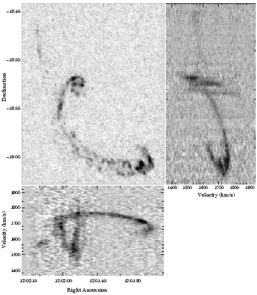
Figure 3.— Three orthogonal projections of the the intermediate resolution H i datacube. The upper left panel shows the sky view, $I(\alpha,\delta)$, and to either side of this are the two orthogonal position-velocity profiles, $I(\alpha,V_{z})$ (bottom) and $I(V_{z},\delta)$ (right). The $(\alpha,\delta)$ view is displayed using a “maximum voxel” function, which displays the value of the brightest pixel along the third ($V_{z}$) dimension (see text). The $I(\alpha,V_{z})$ and $I(V_{z},\delta)$ projections are constructed by summing the emission along one of the spatial dimensions of the datacube, either right ascension or declination. These panels clearly show the well-behaved kinematic structure of the tidal features, as well as the wealth of gaseous sub-structure within the tails and disk.

The maximum voxel display emphasizes regions where the H i  is cold and dense (maximum number of H i  atoms per unit velocity). As a result, it emphasizes the dynamically cold tidal tails. Note especially how the disk H i, which has the highest integrated H i column density, appears fainter in Fig. 3 than in the zeroth moment maps (Fig. 1). This is because the disk gas is spread over a very broad range of velocities. Fig. 3 reveals a number of dense knots within the southern tail, especially toward its end. The maximum voxel display ensures that this is not due to a line-of-sight integration effect where the tail bends back along our line-of-sight. Notice also that similar dense knots are not found within the northern tail. The southern tail also exhibits an interesting parallel or “bifurcated” structure that starts where the southern tail begins to bend westward, and joins back together just before the location of the star forming regions identified by Mirabel et al. (see Fig. 6 for the precise location of the star forming regions).

The tail structure and kinematics are further illustrated in the channel maps, shown in Figure 4 (low resolution data after Hanning smoothing by a factor of two in velocity to $\Delta v$=10.6 km s^-1, contoured upon the optical) and Figure 5 (intermediate resolution data; $\Delta v$=5.2 km s^-1, shown as a greyscale). Only channels containing emission from the tidal tails are shown in these figures, as the disk emission is spread over a much broader range of velocities and are shown separately below (§3.5). Fig. 4 gives a more complete mapping of the gas within the tidal tails and shows its relationship to the underlying starlight, while Fig. 5 allows a more detailed view of the structure of the gas within the tails.

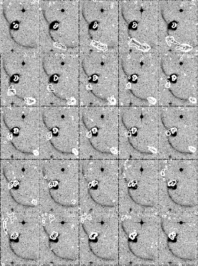
Figure 4.— H i  channel maps of the tidal regions of NGC 4038/9 contoured upon the blue DSS image. The more sensitive low resolution H i cube is used after smoothing by a factor of two in velocity (to a 10.6 km s^-1 channel width). The 40^′′ beam size is indicated in the lower left hand corner of the first panel, and each panel is labeled with its heliocentric velocity. Contours are drawn at levels of (3, 6, 12, 24, …) $\times$1.1 mJy beam^-1, where 1.1 mJy beam^-1 is the single channel noise level, corresponding to a column density of 8$\times 10^{18}\,{\rm cm}^{-2}$. Only channels showing H i emission from the tails are shown.

The greyscale representation of the channel maps in Fig. 5 clearly shows the “bifurcated” morphology of the southern tail mentioned above. The bifurcation is particularly apparent in the channels between 1760 and 1734 km s^-1. The two filaments merge together in a sideways “V” shape in the vicinity of the star forming regions identified by MDL92 (panel at 1734 km s^-1 in Fig. 5). The outer (southern) filament is associated with the previously described high $M_{HI}/L_{B}$ material that lies off of the optical tail (see also panels at 1729 – 1772 km s^-1 in Fig. 4). The inner (northern) filament projects onto the optical tail and has a higher characteristic column density.

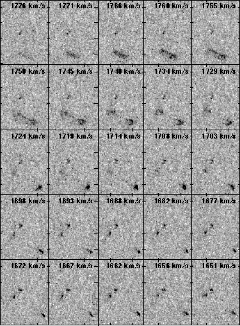
Figure 5.— A greyscale representation of the intermediate resolution H i channel maps of the tidal regions of NGC 4038/9. The greyscales are saturated at 1.1$\times 10^{20}\,{\rm cm}^{-2}$. Each panel is labeled with its heliocentric velocity. Only channels showing H i emission from the tails are shown. This figure emphasizes the wealth of gaseous structure present in the tidal regions.

3.2. Northern Tail Morphology

The low resolution moment map (Fig. 1) shows that the northern H i  tail extends beyond the end of the optical tail, to a projected radius of 7$\farcm$3 (40 kpc) from the center of NGC 4039. This extension is confirmed by the ATCA observations of Gordon et al.  (2001). We detect a total of 4.2$\times 10^{8}M_{\odot}$ of H i  associated with the northern tail, which is much more than found in any of the previous observations. The northern tail is redder (Fig. 2b), less luminous, and has a lower relative H i content than the southern tail (Table 3).

We also notice that the gas in the northern tail is relegated to the outer half of the optical tail and in a purely gaseous extension beyond this. In particular, there is a distinct gap in the H i distribution from a projected radius of 25 kpc back to where the tail connects onto NGC 4039. The difference in the H i  content of the tails appears to be mirrored in the quantities of H i  within the disks associated with either tail (with NGC 4038 being gas rich and NGC 4039 being gas poor; see §3.5 below). These differences and the lack of H i  at the base of the northern tail were already noted by van der Hulst (1979a), who attributed them to a difference in the H i  content of the parent galaxies. We will return to this point in §4.1

3.3. Global Tail Kinematics

Velocities along the northern tail show a regular gradient from 1610 km s^-1  at the base of the H i  to 1540 km s^-1  at the end of optical tail, while the velocities along the southern tail range from 1590, where the tail connects onto the northern disk, to a peak of 1770 km s^-1  midway along the tail, declining to 1610 km s^-1  toward the tip. This kinematic continuity is convincingly illustrated in the position-velocity plots in Fig. 3, which also demonstrates that the tidal gas is quite dynamically cold. The smooth run of velocities along the tails is already apparent from the Westerbork data of van der Hulst (1979a), and is expected from tidal interaction models (e.g. Barnes 1988, Hibbard & Mihos 1995).

The well-behaved kinematics enable us to infer the approximate tail geometry. For example, along the southern tail the H i column density is lowest at the regions of the most extreme redshift, and increases to either side of this. This indicates that this region of the tail lies perpendicular to our line-of-sight, with its motion directed most nearly toward us. At this location, the tail has a minimum projected thickness and hence lowest H i column density. To either side of this the tail curves toward our line-of-sight, resulting in a larger pathlength through the gas-rich tidal material and hence a higher projected column density. The sharper velocity gradients to either side reflect the slewing of the velocity vectors as the tail bends away from us. Similarly, the sharp up-turn at the end of the southern tail in both space and velocity suggests that this region curves away from us. We will address the implications of this geometry for any embedded tidal dwarf galaxy in §3.4.

Since tails are kinematically expanding structures (Toomre & Toomre 1972, Barnes 1988), the relative velocities of the two tails indicate that the southern tail is moving away from us and connects back to NGC 4038 from behind while the northern tail is swinging slightly toward us and connects back to NGC 4039 from the front. This geometry is supported by the lack of a dust absorption feature associated with the southern tail as it crosses from the south back to NGC 4038. In fact, the optical colors of these regions are quite blue (Fig. 2b), whereas we would expect red colors from dust absorption if this gas-rich material lies between us and the disk. As shown directly by van der Hulst (1979a), these kinematics are consistent with the prograde spin geometry derived by the early numerical models of this system by Toomre & Toomre (1972; see also Barnes 1988; Mihos, Bothun & Richstone 1993).

Following the southern tail kinematics back to its progenitor disk (NGC 4038, to the north), we see that the velocities become blueshifted toward the base of the tail (Fig. 3). Since the predominantly redshifted velocities of the tail constrain it to be swinging away from us and connect back to the disk of NGC 4038 from behind, the blueshifted velocities at the base indicate material that is streaming back toward the disk from the tidal tail (Hibbard et al.  1994). Such streaming is a natural consequence of such encounters (e.g. Barnes 1988, Hernquist & Spergel 1992, Hibbard & Mihos 1995), and arises because the tail material at smaller radii is more tightly bound than material further out. As a result, this material reaches its orbital apocenter more quickly and subsequently falls back toward the inner regions.

We can use the maximum projected tail length of 65 kpc and the disk rotation speed inferred from the Fabry-Perot observations of Amram et al.  1992 (155 km s^-1, corrected for disk inclination), to infer an interaction age (measured from orbital periapse, when the tails were launched) of 420 Myr. This is in excellent agreement with the best-match time of 450 Myr from the numerical model of NGC 4038/9 run by Barnes (1988). It is also remarkably close to the age of the population of 500 Myr old globular clusters found by Whitmore et al. (1999; see also Fritze-v.Alvensleben 1998), supporting the hypothesis that this GC population formed around the time when the tails were first ejected (Whitmore et al. 1999).

From Fig. 2d we note that the velocity dispersion within the tidal tails is actually quite low: except for the base of the southern tail, the H i dispersion is less than 16 km s^-1, and the mean of 7 km s^-1 is typical of values measured in undisturbed disk galaxies. This is true of long-tailed mergers in general (Hibbard & van Gorkom 1996, Hibbard & Yun 1999a). The dispersion near the base of the southern tail has higher characteristic values of 13–25 km s^-1. These regions likely lie along a steeper gradient in the potential, and are also regions where the line-of-sight velocities are changing rapidly (Fig. 2c). These effects will lead to larger real and apparent velocity gradients, increasing the single-beam dispersion.

3.4. The Tidal Dwarf Galaxy Candidates

The improved resolution of the VLA observations allows us to directly address the behavior of the atomic gas in the vicinity of the putative tidal dwarf galaxy(s) identified near the end of the southern tail of The Antennae. We show a close-up of this area in Figure 6, which has the same arrangement as the panels in Fig. 2.

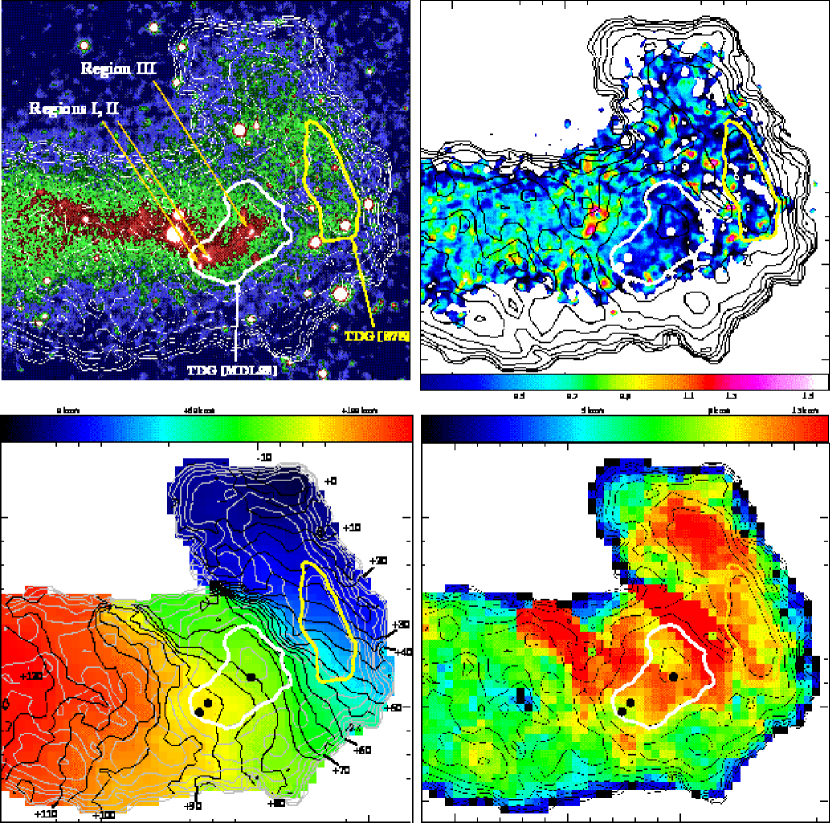
Figure 6.— Four-panel mosaic of the region of the putative Tidal Dwarf Galaxy. The upper left panel shows the optical image in false color, with contours from the intermediate resolution H i data drawn at levels of 14.44 Jy km s^-1 (5$\times 10^{19}\,{\rm cm}^{-2}$) $\times 1.5^{n}$, $n=1-9$. These contours are repeated in all panels. The three star forming regions identified by Mirabel et al. (1992) are labeled in the upper left panel, and are indicated by black or white dots in subsequent panels. Solid heavy contours delineate the approximate half-light level around the Tidal Dwarf candidates identified by Mirabel et al. 1992 (heavy white contour labeled TDG [MDL92]) and by Schweizer 1978 (heavy yellow contour labeled TDG [S78]). The upper right panel shows a color representation of the $B-R$ color map, with the same color mapping as in Fig. 2b. The lower left panel shows the intensity weighted H i velocities with isovelocity contours drawn in black at 5 km s^-1 intervals. The lower right panel maps the H i velocity dispersion, with the same color mapping as in Fig. 2d.

Schweizer (1978) was the first to identify four H ii regions and blue $UBV$ colors associated with the end of the southern tail. He also identified a patch of low surface brightness material bending sharply to the north after the end of the optical tail, which he suggested was a separate dwarf stellar system. We indicate the approximate location of this candidate TDG in Fig. 6 using a thick yellow contour drawn at approximately one half of the local peak H i column density after background subtraction and labeled TDG [S78]. Schweizer noted that in the low-resolution H i map of van der Hulst (1979), the H i appears to be more closely concentrated in the low surface brightness extension of the tail, and hypothesized that the dwarf may have been created during the interaction, as envisioned by Zwicky (1956).

The end of the tail was subsequently studied by Mirabel et al. (1992), who concentrated on what they called a “detached condensation of gas and stars at the tip of a tidal tail”, consisting of a twisted stellar bar embedded in an envelope of diffuse optical emission and containing three emission line complexes. We indicate the approximate location of this candidate TDG in Fig. 6 using a thick white contour drawn at approximately one half of the local peak H i column density after background subtraction and labeled TDG [MDL92]. The three star forming regions identified by MDL92 are labeled as Regions i–iii in Fig. 6a, and are represented by black or white dots in the remaining panels.

While all subsequent observers have referred to the region identified by MDL92 when discussing the putative TDG, we will address the dynamical nature of both of these regions. This is not a trivial task, as the precise boundaries of the TDG candidates have never been explicitly defined.

Our H i observations (as well as those by Mahoney et al. 1987 and Gordon et al. 2001) are a vast improvement on the observations of van der Hulst (1979), and show that the tail is a continuous kinematic structure. Specifically, there is no “detached” region which can readily be identified as a distinct entity. Further, the velocity field varies smoothly through the region containing the high gas column densities and star forming regions without a significant twist or kink. The strongest velocity gradient corresponds with the region where the tail turns abruptly to the north (compressed contours near the center of the map in Fig. 6c, with a similar gradient just to the east of this). This smooth gradient suggests that the velocity field in this region is dominated by projection effects, with the tail bending away from us back into the plane of the sky; as a result the velocity vector slews from pointing toward us to pointing away from us. Therefore, we find no clear kinematic evidence in the velocity field for any dynamically distinct entities. It is possible that the strong tidal gradient may mask the kinematic signature of any mass concentration.

Since there are no well defined boundaries to the dwarf candidates, we calculate the H i mass and blue luminosity in their vicinity by summing the emission within successive circular apertures centered on the local H i column density peaks. The maximum aperture radius is set by the half-width of the tail. A mean background is subtracted, and the H i flux is summed within each aperture of radius $R$. The optical luminosity is measured from the smoothed star-subtracted $B$-band within the same apertures.

The results of these calculations are shown in Fig. 7. The left panel shows the result for TDG [MDL92] and the right panel shows the result for TDG [S78]. In these plots, the solid and dashed lines show how the H i mass and blue luminosity grow as a function of the aperture radius $R$. In Table 4 we list the total H i mass and optical luminosity measured by these curves for each dwarf candidate, but since there are no distinct boundaries for either region, these values should be considered very rough guides.

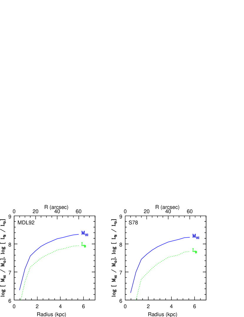
Figure 7.— Results of luminous mass calculation for the candidate Tidal Dwarfs identified by Schweizer 1978 (right panels, labeled TDG [S78]) and by Mirabel et al. 1992 (left panels, labeled TDG [MDL92]). On both cases, the origin is taken to be the peak gas surface density in the integrated intensity map (see Fig. 6). The two curves show the enclosed H i mass (solid curve) and optical luminosity (dashed curve) as a function of the circular aperture radius $R$.

The strong velocity gradients mentioned above give rise to the regions with the highest H i velocity dispersions in Fig. 6d, as gas with different space velocities fall within the same beam. Aside from these regions, there are other local peaks in the gas velocity dispersion which might provide possible evidence for a mass concentration: between Regions i & ii and Region iii the H i velocity dispersion increases to $\sim$12 km s^-1 vs. an average of 6–7 km s^-1 along the tail. Similar signatures are seen at the location of tidal dwarf candidates within the optical tails of the merger remnants NGC 7252 (Hibbard et al. 1994) and NGC 3921 (Hibbard & van Gorkom 1993, 1996). However, it is noteworthy that the three H ii regions actually fall on the edges of H i maxima. Similar signatures are seen near giant H ii regions in dwarf galaxies (e.g. Stewart et al. 2000, Walter & Brinks 1999), where the increased H i linewidth is due instead to kinetic agitation of the gas from energy deposited by young stars, SNe and stellar winds (e.g. Stewart et al. 2000, Yang et al. 1996, Tenorio-Tagle & Bodenheimer 1988 and references therein) rather than the gravitational effects of a mass concentration.

There is also an increased dispersion to the north of TDG [S78] (dispersion increases to 15.6 km s^-1 over the surrounding value of 11 km s^-1). However, an examination of the line profiles shows that the increased dispersion comes from low-level emission spread over many channels. Adjacent regions have this broad low-level component, but also have a brighter narrower component which leads to a lower intensity-weighted line-width. So we do not believe that this is a signature of a mass concentration at this location.

Since the moment maps are susceptible to line-of-sight integration effects, we turn to the velocity cubes directly for further insight. From the channel maps, we find that the gas near the TDG obtains the highest gaseous phase-space densities in this system (i.e. density enhancements localized in space and velocity). In fact, this region has a higher H i column density per unit km s^-1 than any other region in this system, including regions within the disk or overlap region (see also Fig. 3a). The peak of 21 mJy beam^-1 in a single velocity channel of width 5.2 km s^-1 corresponds to a single channel column density of 3.8$\times 10^{20}\,{\rm cm}^{-2}$, and the integrated column density of 1.3$\times 10^{21}\,{\rm cm}^{-2}$ represents an enhancement of 6 over the mean tail density. The high-resolution data shows an even higher single-channel peak of 6.4$\times 10^{20}\,{\rm cm}^{-2}$.

A closer examination shows that there are actually two dense knots in this region. These are seen in the channel maps from the intermediate resolution datacube, plotted at full velocity resolution in Fig. 8. The densest concentration appears at $V$=1708 km s^-1  and lies just north of star forming Region iii. The second concentration encompasses star forming Regions i & ii and appears at $V$=1719–1729 km s^-1. Such concentrations suggest regions of gaseous dissipation. While this is not unequivocal evidence of a self-gravitating dwarf-sized object, since increased gaseous dissipation is expected in regions of recent star formation, it does indicate that there is something unique about this region of the tail.

Figure 8.— H i  channel maps of the region around the putative Tidal Dwarf Galaxy within the southern tail of NGC 4038/9 contoured upon a greyscale representation of the $B$-band image. The greyscales range from $\mu_{B}$=28.5 mag arcsec^-2  (white) to 25 mag arcsec^-2  (black). The intermediate resolution H i  cube is used at its full velocity resolution (5.2 km s^-1  channel width). Contours are drawn at levels of 2.8 mJy beam${}^{-1}\times 1.5^{n},n=0-4$, where 2.8 mJy beam^-1 corresponds to a single channel column density of 5$\times 10^{19}\,{\rm cm}^{-2}$.

The channel maps also show the bifurcated structure mentioned in §3.1. It is very interesting that the two parallel filaments join just east of the location of the star forming regions associated with the TDG (the “V”-shaped feature seen in the panel at 1734 km s^-1 of Fig. 8). Again, these observations suggest that there is something special about the gas and tail geometry at the location of the star forming regions.

The parallel filaments can be seen separately in the channels from V=1755–1724 km s^-1. The northern filament quite clearly lies along the optical tail, while the southern filament is displaced by about 8 kpc to the south. The density peaks are of similar magnitude in either filament, but only at the location of the putative TDG is there a corresponding increase seen in the optical light underlying the gas peaks. The gas concentration associated with Region iii appears to lie within the northern filament, while it is difficult to say whether the concentration associated with Regions i & ii are associated with one filament or the other. At velocities below 1693 km s^-1, it appears that only the southern filament continues on to the gas rich “hook” at the end of the tail.

Fig. 2b shows that the blue tail colors discovered by S78 are not restricted just to the high column density gas near either TDG, but represents a trend of increasing blueness with distance along the tail. We find that while the outer disks and southern tail have similar $B-R$ colors, the end of the southern tail is bluer in $V-R$ than $B-V$ while the reverse holds for the outer disks. This suggests that the tail material is younger and/or more metal poor than the outer disk material (Schombert et al. 1990, Weilbacher et al. 2000), although we postpone to a later paper a full color analysis (Evans et al. 2001).

3.5. Disk Morphology and Kinematics

Fig. 9 shows an overlay of the high resolution H i contours upon a false-color representation of the $B$-band image (Fig. 9a), of the $B-K$ color map (Fig. 9b), of the H i velocity dispersion map (Fig. 9d), and of the NIR $K$-band image (Fig. 9e). In Fig. 9c we show a color representation of the H i velocity field with isovelocity contours drawn at intervals of 5 km s^-1. Finally, in Fig. 9f we show the integrated CO map of Wilson et al. (2000) contoured in green upon a greyscale representation of the H i column density. The latter image gives a better idea of the local minima and maxima in the H i distribution, as these are not always self-evident in the contour map. In this panel red crosses indicate the location of the “Super Star Clusters” (SSCs) identified in the HST image of Whitmore et al. (1995, from their Table 1).

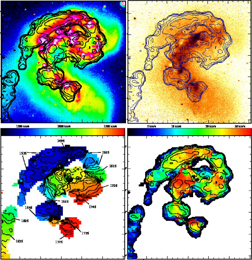
Figure 9.— Details of the H i  emission within the disks of NGC 4038/9. The upper left panel shows contours from the high resolution H i  datacube ($11.4^{\prime\prime}\times 7.4^{\prime\prime}$) upon a false-color representation of the $B$-band image. Contours are drawn at levels of (1, 2, 4, 8, …) $\times$7.74 mJy beam^-1 km s^-1, where the lowest contour corresponds to a column density of 1$\times 10^{20}\,{\rm cm}^{-2}$. The upper right panel shows the same H i contours upon the $B-K$ color map, where lighter shades indicate bluer colors and darker shades represent redder colors. The middle two panels show the intensity weighted H i velocities with isovelocity contours drawn at 5 km s^-1 intervals (left) and the H i velocity dispersion with the same H i contours as in the first panel (right). The next two panels shows $K$-band image with the H i contours superimposed on the left, and the a greyscale representation of the H i image on the right, with the CO contours of Wilson et al. (2001) superimposed and red crosses marking the location of the Super Star Clusters identified by Whitmore & Schweizer (their Table 4).

In Fig. 9b dark regions represent the reddest $B-K$ colors, generally indicating regions of high dust extinction, while light regions represent the bluest colors, generally indicating unobscured massive young stars. Comparison of Figs. 9b & f shows that the CO is closely associated with the red features in the $B-K$ map, so that the CO traces the dust distribution.

Figs. 9b & f show that on a global scale, the H i distribution traces both the regions containing the most star clusters and the regions with the highest dust content, e.g. the star forming ring in NGC 4038 and the star forming half of the disk of NGC 4039 (to the northeast of the nucleus), and the dusty region between the two galaxies and to the southwest of NGC 4039. On finer scales (i.e. of order a few kpc), the H i is not particularly associated with the bluest star clusters or reddest dust concentrations. Most of the SSCs in Fig. 9f actually appear to lie along steep gradients in the H i and CO distributions. The molecular gas peaks are often displaced from the $N_{HI}$ peaks and many of the SSCs actually lie in the transition zone between the two gas phases. Where there are no displaced CO peaks, the SSCs still lie predominantly along steep gradients in the H i distribution.

The NIR image in Figs. 9b does not show additional light peaks in the regions of highest H i column density (recall that dust extinction is 10 times weaker in the NIR compared to the optical), so we conclude that the occurrence of SSCs along gradients in the H i distribution is not due to dust associated with the H i  obscuring clusters at the regions of highest H i  column density. Rather, we suspect that it is due to young stars ionizing or sweeping the H i  on the one hand, and the conversion of H i  to molecular form on the other. We refer the reader to Zhang, Fall & Whitmore (2001) for a much more thorough discussion of the relationship between SSC’s of various ages and the H i, Radio continuum, CO, X-ray, FIR, MIR, $H\alpha$ and optical morphology and the H i and CO kinematics.

The lower H i contours in Fig. 9 are very close together, with the H i column density falling off sharply below 4$\times 10^{20}\,{\rm cm}^{-2}$. The western part of the disk of NGC 4038 is largely devoid of H i, as is most of the extended disk of NGC 4039. Examination of the lower resolution H i maps (Figs. 1, 2a) shows that this is true even at lower H i column densities. Probably not coincidently, these regions lack current star forming regions.

The intensity weighted H i velocities of NGC 4038/9 (Fig. 9c) shows a very disturbed velocity field, similar to those mapped in H i (Gordon et al. 2001) H$\alpha$ (Burbidge & Burbidge 1966, Rubin et al. 1970, Amram et al. 1992) and in CO (Stanford et al. 1990, Wilson et al. 2000, Zhu 2001). In particular, the disk of NGC 4038 has a north-south gradient spanning $\sim$ 250 km s^-1, while NGC 4039 has a northeast-southwest gradient spanning a similar range (see also Fig. 3). The general sense of motion — north blueshifted, south redshifted — agrees with the sense of rotation inferred from the tidal tail. However, because of the extremely disturbed nature of both disks, the kinematics of these regions are not simply rotational. It is likely that there are strong streaming motions along the star forming loop and along the overlap region connecting the two disks.

In Figure 10 we present the disk channel maps, made from the intermediate resolution data after Hanning smoothing by a factor of four in velocity ($\Delta v$=20.4 km s^-1). Instead of a normal rotational pattern, the redshifted gas concentration to the SW of NGC 4039 shows very little spatial gradient over the velocity range V=1836–1708 km s^-1, while the blueshifted gas to the northeast of NGC 4039 has very little spatial gradient over the velocity range V=1579–1472 km s^-1. The gas not associated with either of these two regions appears to flow from the NE at V=1558 km s^-1 to the SW at V=1665 km s^-1. This is likely material which is flowing along the overlap region between the two galaxies. The H i in the northeast part of NGC 4039 may be material which is being accreted from NGC 4038 along the bridge connecting the two systems. We also notice that the disk gas connects smoothly to the gas associated with the base of the southern tail (channels at V=1472–1686 km s^-1). From the tail kinematics (§3.3) we concluded that the blueshifted velocities associated with the base of the tail require that this gas streams back onto the outer disk of NGC 4038 from the tail. In Fig. 9d we find a region of high velocity dispersion along the northern loop of gas (dispersion of 28 km s^-1 vs 22 km s^-1 at adjacent regions). We suggest that this increase is associated with gas falling back from the tail mixing along the line-of-sight with gas associated with the disk.

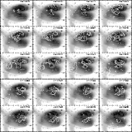
Figure 10.— H i  channel maps of the disk regions of NGC 4038/9 contoured upon the CTIO $B$-band image. The intermediate resolution H i cube is used after smoothing by a factor of four in velocity (to a 21 km s^-1 channel width). Each panel is labeled with its heliocentric velocity. Contours are drawn at levels of (-3, 3, 6, 12, 24, …) $\times$0.4 mJy beam^-1, where 0.4 mJy beam^-1 is the rebinned channel noise level, corresponding to a column density of 3$\times 10^{19}\,{\rm cm}^{-2}$. These maps show the entire velocity spread of the present observations, and the reader should refer to Gordon et al. (2001) for H i emission from the disk regions that falls outside of our bandpass.

3.6. The Nearby Dwarf Galaxy ESO 572–G045

As part of this observation we also detect H i  associated with the Scd dwarf galaxy ESO 572–G045 just to the southwest of the tip of the southern tail (5.7^′ or 32 kpc from the TDG). This system lies at a projected distance of 90 kpc from The Antennae. This galaxy is very flattened, with an axis ratio near 10, associating it with the class of “superthin” galaxies (Goad & Roberts 1981), and qualifying it for membership in the “Flat Galaxy Catalogue” of Karachentsev et al. (1993). It is curious that a similar superthin galaxy was also serendipitously discovered by Duc et al. (2000) in their HI mapping of the interacting system NGC 2992/3, another interacting pair with a candidate Tidal Dwarf within a gas-rich tidal tail.

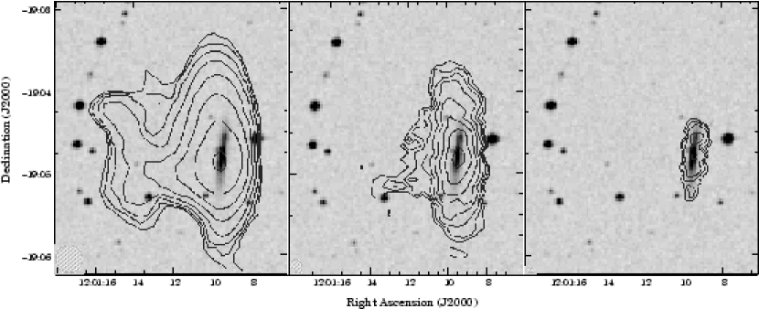
Figure 11.— Contours of the integrated H i  emission of the small superthin galaxy ESO 572–G045 overlaid on the DSS image. These panels show the H i  data from the low– (left), intermediate– (middle) and high– (right) resolution datacubes, with the beam size of each dataset drawn in the lower left corner. Contours are drawn at levels of [144.9 Jy km s^-1 $\times$$2^{n/2}$, 57.75 Jy km s^-1 $\times$$2^{n/2}$, 18.1 Jy km s^-1 $\times$$2^{n}$] ($n=0,1,2...$), for the low, intermediate and high-resolution data, respectively. The lowest contour corresponds to a column density of [1$\times 10^{20}\,{\rm cm}^{-2}$, 1$\times 10^{20}\,{\rm cm}^{-2}$, 4$\times 10^{20}\,{\rm cm}^{-2}$], respectively. Notice the gaseous extensions extending to the east in the intermediate and low resolution maps.

Contours of the H i column density from the various resolution data cubes are shown on the optical image from the DSS in Figure 11. We detect a total 3.7$\times 10^{8}M_{\odot}$ of H i spread over 100 km s^-1 and extending to a radius of 6 kpc (i.e., twice as far as the optical light). The galaxy is nearly edge-on and shows a linear velocity gradient. Assuming an edge-on orientation and circular velocities (with $V_{circ}$ = 50 km s^-1), this suggests a dynamical mass ($M_{dyn}$) of 3.5$\times 10^{9}M_{\odot}$ out to 6 kpc. Using the optical properties given in NED (major and minor axis of $1.01^{\prime}\times 0.11^{\prime}$ and $m_{B}=$16.70 mag), we derive dimensions of 5.9 kpc $\times$ 0.6 kpc and a luminosity of $L_{B}=1.9\times 10^{8}L_{\odot}$. This system is quite gas rich ($M_{HI}/M_{dyn}=0.11,M_{HI}/L_{B}=1.9$), with global properties similar to those of other superthin galaxies (Matthews et al. 1999).

The low resolution H i map in Fig. 11a clearly shows some low column density gas extending to the east. Since this extension is one-sided in nature, it is more indicative of ram pressure effects than tidal effects. The very thin and flat disk of ESO 572–G045 also argues against significant tidal forces acting on it. This suggests that there may be an extended warm or hot gaseous halo around NGC 4038/9 that is affecting the diffuse cold ISM of ESO 572–G045 (e.g. Moore & Davies 1994).

4. Discussion

The wealth of information provided by these observations is a testament to the utility of H i  spectral line mapping of disturbed systems. While in some sense the present data are just the beginning point of many more involved investigations, particularly for dynamical modeling of this system, they also lead to many interesting results on their own, which we discuss in this section.

4.1. The lack of H i  at the base of the Northern Tail

The difference between the northern and southern tail in both optical structure and H i  content was already noted by van der Hulst (1979a), who attributed it to a difference in the H i  content of the parent galaxies. The lack of H i  within the main disk NGC 4039 (i.e. the progenitor of the northern tail) was seen as support for this interpretation. However, we now feel that the observations are at odds with this explanation. For while it is true that the outermost regions of tidal tails should originate from the outermost regions of the progenitor disks, it is not true that the outermost regions of the progenitor disks end up only at the outermost regions of tidal tails. In fact, this gas rich material should extend all the way back to the host system. This fact is apparent already in the simple models and illustrations of Toomre & Toomre 1972 (see their Fig. 2). This reflects the fact that tails are not linear structures, but actually two dimensional “ribbons” twisting through space, with the outer disk material forming a “sheath” around the inner disk material (Mihos 2001). As a result, the gas rich outer regions should extend along the entire length of the tidal feature back toward the progenitor disk. It therefore seems that a low H i  gas content alone cannot explain the gas-rich outer tail and gas-poor inner tail.

In a recent paper, Mihos (2001) describes a kinematically decoupling between the gaseous and stellar components of a tail that occur during tail formation. However, this decoupling leads to a displacement between the gaseous and stellar tidal features, and does not totally remove large quantities of gas from along radial segments of the tail. It is unlikely, therefore, that this mechanism explains the present observations.

Hibbard, Vacca & Yun (2000) investigate several possible mechanisms for creating differences between H i and optical tidal morphologies. Two plausible mechanisms are ram-pressure stripping of the tidal gas from an expanding superwind and ionization of the gas by UV photons escaping from the starburst. While there is some evidence for a nuclear outflow in NGC 4038/9 (Read, Ponman, & Wolstencroft 1995, Sansom et al. 1996, Fabbiano, Schweizer & Mackie 1997, Lipari et al. 2001, Fabbiano, Zezas & Murray 2001), the soft X-ray morphology (Read et al. 1995, Fabbiano et al. 2001) does not suggest that this wind is directed toward the northern tail, so we concentrate instead on possible ionization effects.

The situation explored by Hibbard et al.  (2000) is that the starburst has cleared enough dust and gas from the inner regions to provide direct unobscured sightlines to the tails. By equating the surface ionization rate with the recombination rate, they find that the gas should be ionized out to a distance given by:

$$R_{ionized} \leq 25\,{\rm kpc}\,\left({f_{esc}\over 0.05}\right)^{1/2}\left({L_{IR}\over 6\times 10^{10}L_{\odot}}\right)^{1/2}$$ (1)

$$\times \left({2\times 10^{20}{\rm cm}^{-2}\over N_{HI}}\right)\left({dL\over 5\,{\rm kpc}}\right)^{1/2}$$

Where $N_{HI}$ and $dL$ are the column density and thickness of the H i layer being ionized, $f_{esc}$ is the fraction of ionized photons emerging from the starburst, and we have made the standard assumption that most of the starburst luminosity is emitted in the far infrared (see Hibbard et al.  2000 for details).

The fiducial values used in eqn. 1 are appropriate for NGC 4038/9, and we thus find that the starburst may well be capable of ionizing gas out to the H i base of the northern tail (25 kpc projected radius), providing the tail has a clear sightline to the ionizing stars and that $f_{esc}$ is not much smaller than 0.05. Evidence that $f_{esc}$ is at least as large as this is provided by numerical work by Dove, Shull & Ferrara (2000), who derive $f_{esc}\sim 0.1$ for normal galaxies, and suggest that starbursts should have significantly higher values. Hurwitz, Jelinsky, & Dixon (1997) find upper limits to the escape fraction of $UV$ photons of 3–57% for four IR luminous starbursts, while Bland-Hawthorn & Maloney (1999) calculate $f_{esc}=0.06$ for the Milky Way (see discussion in Bland-Hawthorn & Putman 2001).

So the question becomes, is it likely that the northern tail of NGC 4039 has a relatively clear view of the star-forming disk, while the southern tail does not? We believe the answer to this question is yes. The majority of the unobscured massive star forming regions in NGC 4038/9 are associated with the disk of NGC 4038 and the material along the bridge (Whitmore & Schweizer 1995, Whitmore et al. 1999). Since tidal tails are spun off close to the spin plane of the progenitor (Toomre & Toomre 1972), the southern tail will not have a clear view to the star forming regions located within the disk NGC 4038, and the body of NGC 4039 would block ionization originating from the bridge star forming regions. The body of NGC 4039, on the other hand, appears to have a perfect view of the star forming disk of NGC 4038 and the northern tail should have a view to the backside of this disk. This prediction can be tested by numerical models to constrain the space geometry of the tail.

We suggest that NGC 4039 had a normal H i  distribution, but that much of this gas has been photoionized by the starburst. We believe a similar effect is responsible for the lack of H i  at smaller radii in the otherwise gas-rich tidal tails of the NGC 7252, Arp 105, and Arp 299 systems (Hibbard, Vacca & Yun 2000). If this is indeed the case, then the ionized gas should be visible via its recombination radiation. Using the equation given in Hibbard et al. (2000), the expected emission measure of this radiation should be $EM=0.8\,{\rm cm^{-6}\,pc}$ for a gas column density of 2$\times 10^{20}\,{\rm cm}^{-2}$ and thickness of 5 kpc. This is within the capabilities of modern CCD detectors (e.g.  Donahue et al.  1995; Hoopes, Walterbos & Rand 1999).

4.2. The Bifurcation of the Southern Tail

As mentioned above, tails are two dimensional “ribbons” twisting through space. It is possible that a lateral twist may cause the outer edge of the ribbon to lie in a different plane from the inner regions, i.e. for the most gas-rich (highest $M_{HI}/L_{B}$) regions to appear in a different plane from the less gas-rich but optically brighter regions (Mihos 2001). In Hibbard & Yun (1999a) we suggest that this this effect may be exacerbated by a pre-existing warp in the progenitor disk, providing even more marked offsets. This provides a simple explanation for the gas-rich but optically faint outer edge of the southern tail. Similar bifurcated tails are seen in several systems (e.g. M81, van der Hulst 1979b, Yun et al.  1994; NGC 3921, Hibbard & van Gorkom 1996; NGC 2535/6, Kaufman et al.  1997; Arp 299 Hibbard & Yun 1999a).

What is intriguing is that the two filaments appear to join back together just at the location of the star forming regions associated with the candidate tidal dwarf TDG [MDL92] (the “V”-shape seen in Figs. 5 & 8 and discussed in §3.1 & §3.4). We do not know whether this is a coincidence or an important clue. Further insight into this question will have to await a more detailed numerical study of this system.

4.3. The Formation of the Tidal Dwarf Galaxy

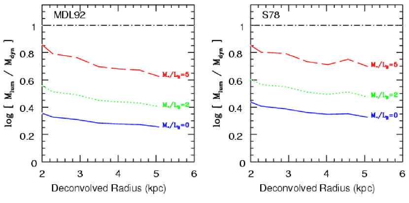
Figure 12.— Results of dynamical analysis for the candidate Tidal Dwarfs identified by Schweizer 1978 (right panels, labeled TDG [S78]) and by Mirabel et al. 1992 (left panels, labeled TDG [MDL92]). On both cases, the origin is taken to be the peak gas surface density in the integrated intensity map (see Fig. 6). We plot $M_{lum}/M_{dyn}$ as a function of the deconvolved aperture radius $r$. Three curves are drawn, each one representing a different stellar mass-to-light ratio: the thick solid curve shows the result for $M_{*}/L_{B}=0$ $M_{\odot}\,L_{\odot}^{-1}$, the dotted curve shows the results for $M_{*}/L_{B}=2$ $M_{\odot}\,L_{\odot}^{-1}$, and the dashed line shows the results for $M_{*}/L_{B}=5$ $M_{\odot}\,L_{\odot}^{-1}$.

We wish to take advantage of the higher spatial and velocity resolution of our H i observations to examine the dynamical nature of material in the vicinity of the TDG candidates. This is a difficult task, since there are no distinct objects which can be defined unambiguously. Further, if there are objects within the tail, they are clearly not in isolation, and the kinematics may not be due to the local mass concentration. All of these factors make a clear dynamical analysis fraught with uncertainties. Still, the present data are the best available, in terms of both spatial and kinematic resolution, and this is the nearest system with a candidate tidal dwarf, so we will proceed with all due caution.

The first hypothesis we will test is whether there are concentrations of gas and light centered on the gas peaks with enough mass in luminous matter alone to account for the measured H i line-width. To this end, we compare the virial mass inferred from the H i linewidth ($M_{vir}$) to the total luminous mass inferred from the H i flux and the optical luminosity ($M_{lum}$). A value of $M_{lum}/M_{vir}=0.5$ is sufficient for a region to be bound, while a value of $M_{lum}/M_{vir}=1$ is required for the region to be virialized.

To calculate the virial mass, we must make some assumptions about the 3-dimensional structure of any mass concentration. For the sake of simplicity, we assume that there is an isotropic spherical mass concentration of constant density. For this situation, the virial mass is given by $M_{vir}=3\sigma^{2}\times ar_{h}/G$, where $G$ is the gravitational constant, $\sigma$ is the one-dimensional velocity dispersion, $r_{h}$ is the projected half-light radius, and $a$ is a geometric factor (Binney & Tremaine 1987) $\simeq 2.74$ for the adopted geometry. We take the velocity dispersion at the location of the peak column density, and use the deconvolved half-light radius found from fitting a Gaussian plus constant background to the H i mass distribution.

The luminous mass is calculated from the observed mass and optical luminosity following the prescription given in Paper II. In particular, the possible contribution to the luminous mass by stars is estimated by adopting a range of stellar mass-to-light ratios ($M_{*}/L_{B}$) representing different star formation histories (SFHs). The gas mass is derived from the H i mass by multiplying by a factor of 1.36 to take into account a primordial abundance of Helium. No correction is made for the presence of molecular gas since recent CO observations at the location of the TDG by Gao et al. (2001) and Braine et al. (2001) find only trace amounts of molecular gas in the vicinity of the tidal dwarf (4$\times 10^{6}M_{\odot}$).

We evaluate three different stellar mass-to-light ratios, which span a range of star formation histories. We evaluate $M_{*}/L_{B}=$ 0 $M_{\odot}\,L_{\odot}^{-1}$ (i.e., $M_{lum}=M_{gas}$, also appropriate for a young instantaneous burst); $M_{*}/L_{B}=$ 2 $M_{\odot}\,L_{\odot}^{-1}$, corresponding to a constant SFH at an age of 10 Gyr, and $M_{*}/L_{B}=$ 5 $M_{\odot}\,L_{\odot}^{-1}$, representing an exponentially decreasing SFH with a time constant of 4 Gyr at an age of 10 Gyr (see Paper II for more details). The results of the luminous to virial mass calculation are given in Table 4.

The ratios of the luminous to virial mass given in Table 4 are less than one, suggesting that neither mass concentration is virialized. However, they do not rule out the presence of a bound object. They do imply that there is not a sufficient gas density for the regions to be bound by gas alone (i.e., $M_{lum}/M_{vir}\,<\,0.5$ for $M_{*}/L_{B}=$ 0 $M_{\odot}\,L_{\odot}^{-1}$). This contradicts the conclusion reached for this same region by Braine et al. (2001). The reason for this discrepancy is that Braine et al. use the much narrow CO linewidth to calculate a dynamical mass, yet include both H i and stellar light in their luminous mass calculation (as mentioned above, the mass in molecular mass inferred from the CO line flux is negligible compared to the H i). The fact that the H i linewidth is much broader than the CO linewidth argues that a much larger mass concentration is required to bind it, and the Braine analysis is inappropriate. This point is discussed in more detail in Paper II.

A further conclusion from the above analysis is that if the dwarf candidates are bound, they require a significant contribution to the total mass from evolved stars, or they are bound by dark matter. In this case, the calculated values of $M_{lum}/M_{vir}$ are valid only if the H i line-width also characterizes the motion of the stars (and/or dark matter). This is probably not the case, since in normal disks the older stellar populations (i.e., those with higher $M_{*}/L_{B}$ ratios) have a significantly higher dispersion than the gas, by factors of 2–3 (van der Kruit 1988), which would lead to a virial mass estimate a factor of 4–10 higher and $M_{lum}/M_{vir}$ ratios correspondingly smaller. Young stellar populations have a velocity dispersions similar to the cold gas, but also have smaller $M_{*}/L_{B}$ ratios. A measurement of the stellar kinematics and a better estimate of the stellar mass-to-light ratio is needed to be more conclusive. Finally, we note that the expected circular velocity given by $V_{c}^{2}=GM_{lum}/R$ is 20–30 km s^-1. Fig. 6c shows no sign of rotation at this level. We conclude that either TDG candidate may be, but need not be, self-gravitating.

This virial analysis includes many caveats. Primarily, the above analysis implies that we know the ratio $M_{lum}/M_{vir}$ to within a factor of two, and in truth we do not know either quantity to this precision. Further, unless the bound regions are much smaller than the width of the tail, the geometry is unlikely to be spherical, and the velocities are unlikely to be isotropic. Finally, any entrained objects are clearly not in isolation, complicating the virial analysis. We will be addressing these uncertainties using simulated observations of bound objects within N-body tails (Kohring, Hibbard & Barnes, in preparation).

The above analysis depends on a specific geometry and the details of the Gaussian fit to the gas distribution. A more common but even less clear analysis uses a dynamical mass indicator $M_{dyn}\sim\Delta V^{2}\times R/G$, where $\Delta V$ is the FWHM linewidth, $R$ is a radius, and $G$ is the gravitational constant (e.g. Braine et al. 2001). This quantity has the dimensions of mass, but it is not obvious what mass it defines, especially when the radius used is not physically motivated. However, we can use the quantity to see how taking larger or smaller region in the vicinity of either dwarf candidate might affect our conclusions. Specifically, we evaluate how the ratio of the luminous mass to this dynamical mass indicator changes with radius using the circular apertures defined in §3.4 and the light curves given in Fig. 7. In this case, $\Delta V$ is 2.35 times the one-dimensional velocity dispersion, and $R$ is the deconvolved aperture radius. The luminous mass is calculated from the H i mass and optical luminosity as above.

The results of this exercise is shown in Fig. 12. Three curves are drawn, each one representing a different stellar mass-to-light ratio: the solid curve shows the result for $M_{*}/L_{B}=0$ $M_{\odot}\,L_{\odot}^{-1}$, the dotted curve shows the results for $M_{*}/L_{B}=2$ $M_{\odot}\,L_{\odot}^{-1}$, and the dashed line shows the results for $M_{*}/L_{B}=5$ $M_{\odot}\,L_{\odot}^{-1}$. We see that this ratio decreases with larger apertures. Therefore, taking a larger radius will not change the conclusions reached above. Taking a smaller radius might turn up objects with a larger luminous to dynamical mass, but in this case they would have a much smaller mass scale than is usually assumed.

In conclusion, we find no kinematic signature of a distinct dynamical entity within the southern tail, but any signature might be masked by the strong geometric velocity gradients in this region. If there are bound mass concentrations, they require a significant contribution from either evolved stars or dark matter to bind them.

If the lower distance of 13.8 Mpc suggested by Saviane et al. (2001) is correct, then the luminous mass decreases by a factor of 2 while the virial mass decreases by a factor of 1.4, so the luminous to virial mass estimates all decrease by a factor of 1.4, making it less likely that either TDG candidate is a bound object. Additionally, if there are bound regions, the mass scale would be more typical of dwarf Spheroidal galaxies than dwarf Irregulars, and the gaseous concentrations may have more relevance to remnant streams around galaxies than the formation of dwarf irregulars (Kroupa 1998).

If there are dwarf-galaxy sized concentrations forming within the tail, then the present observations appear inconsistent with the tidal dwarf formation scenario suggested by Elmegreen, Kaufmann & Thomasson (1992). In their scenario the velocity dispersion of tidal gas is increased over the pre-encounter value due to the interaction, increasing the Jeans mass in the tidal gas and leading to the formation of dwarf Irr sized objects. As noted in §3.3, the velocity dispersion within the tidal tails of NGC 4038/9 is typical of values measured in undisturbed disk galaxies. This is true of long-tailed mergers in general (Hibbard & van Gorkom 1996, Hibbard & Yun 1999a) and agrees with the expectation from numerical models. The tails form from the dynamically coldest material on the side of the disk opposite orbital periapses, and expand kinematically thereafter. Tails, particularly those of low-inclination prograde encounters, should not and appear not to be significantly kinematically heated by the encounter. And while it is true that an increased velocity dispersion will suppress the formation of low mass objects, it does not follow that it should lead to the collapse of higher mass objects; it simply means that a higher mass is required in order for the concentration to collapse. Therefore, the model of tidal dwarf formation suggested by Elmegreen, Kaufmann & Thomasson (1992) does not appear to apply here.

4.4. Expected Signature of Merger Remnant

A last point that we wish to make is that NGC 4038/9 is clearly an on-going merger experiencing a massive young starburst which is spread throughout the disk of NGC 4038 and the overlap region. And yet, the long tails of NGC 4038/9 suggest that the interaction began in earnest of order 400 Myr previously. This is very similar to the situation in the infrared luminous merger Arp 299 (Hibbard & Yun 1999a). Additionally, the proximity of NGC 4038/9 have allowed the identification of a population of SSCs with ages of $\sim$ 500 Myr (Whitmore et al. 1999) spread throughout the disk region. Clearly, then, merger induced extra-nuclear star-formation began around the time that the tails were launched, has continued until today, and will likely continue until the merger is complete. Therefore, the merger induced “burst” population will be broadly spread throughout the remnant, both spatially and temporarily. While a significant amount of the present gas supply may find its way into the innermost regions of the remnant, it is not clear how much of this gas will be converted into stars. Much of this gas may be expelled in starburst driven superwind (Heckman et al. 1999, Hibbard & Yun 1999b).

Either way, the expected signature of the evolved merger remnant will not be as pronounced as is often assumed (e.g., Mihos & Hernquist 1994, Bekki & Shioya 1997, Silva & Bothun 1998a,b). Instead of a single epoch metal-enriched population confined to the innermost radii of the remnant and surrounded by a uniformly-old metal poor population, there will be stars with an age range of $\sim$ 1 Gyr spread throughout remnant body, with perhaps an inner population of stars formed from whatever gas is not blown out.

5. Conclusions

• We have mapped the H i  in the classical double-tailed merger, NGC 4038/9, “The Antennae”, with unprecedented spatial and velocity resolution. In agreement with other observers (van der Hulst 1979a, Mahoney et al. 1987, Gordon et al. 2001), we find the northern tail to be gas-rich at its tip but gas-poor at its base, the southern tail to be gas rich along its entire length and with a significant enhancement in the gas concentration in the vicinity of the TDG. The tail kinematics are broadly consistent with the interaction geometry inferred from numerical simulations.

• We suggest that the lack of H i  at the base of the northern tail is due to photoionization by UV photons escaping the disk starburst region. If so, the ionized gas should be readily detectable, with and expected emission measure of order 0.8 cm^-6 pc.

• The H i velocity field at the end of the southern tail is dominated by strong velocity gradients which suggest that at this location the tail is bending away from us. The tail velocity gradients may mask the kinematic signature of any self-gravitating condensation in this region.

• It is not clear whether the TDG candidates identified by Schweizer (1978) and Mirabel et al. (1992) are self-gravitating. The observed kinematics suggest that there is not enough mass in gas alone to account for the H i linewidths of the regions we have delineated. Further insight requires a measurement of the stellar velocity dispersion and tighter constraints on the stellar mass-to-light ratio.

• Whether or not the TDG candidate identified by Mirabel et al. (1992) is a self-gravitating entity, it is clear that this concentration of gas, stars, and star forming regions in the tail is unique. At this location the H i column densities per channel are higher than anywhere else in the system, including within the main disks. We believe a clue to the origin of this concentration is that it occurs just after the the “V”-shape where the two filaments connect back to each other occurs just before the location of of the TDG.

• These observations reveal that the “superthin” galaxy ESO 572–G045 is a companion to NGC 4038/9. Our low resolution data show a low column density H i  extension to the east, suggesting that this system may be experiencing ram pressure as it orbits NGC 4038/9.

Table 1VLA Observing Parameters.

Date		1996 Jun 3	1997 Jun 9
Array		D	CnB
Time on Source (hrs)		2.5	6.5
Phase Center ($\alpha$, $\delta$, J2000)		12h 01m 52s	–18∘ 55′ 40′′
Central Velocity (Heliocentric)		1630 km s-1
Primary Beam (FWHM)		30′
Phase Calibrator		1130–148
Flux Calibrator		3C286
Correlator Mode		1A, on-line Hanning
Bandwidth (MHz)		3.125
Number of Channels		128
Channel Separation (km s-1)		5.21
Data set	High Resolution	Medium Resolution	Low Resolution
“Robust”a parameter	-1	+1	+1, Convolved to 40′′
Synthesized Beam
— Major Axis $\times$  Minor Axis (FWHM)	$11.4^{\prime\prime}\times 7.4^{\prime\prime}$	$20.7^{\prime\prime}\times 15.4^{\prime\prime}$	$40^{\prime\prime}\times 40^{\prime\prime}$
— Position angle (east of north)	76∘	24∘	0∘
Noise Level (1$\sigma$)
— Flux Density (mJy beam-1)	1.3	0.9	1.3
— Column Density ($\times 10^{19}\,{\rm cm}^{-2}$ beam-1 ch-1)	8.8	1.6	0.47
— Brightness Temperature (K beam-1)	9.3	1.7	0.49

Table 2CTIO/UH Observing Parameters.

Date	1991 Apr 17/18	1995 Jan 22
Telescope	CTIO 0.9m	UH 88′′
Camera	Tek 512	QUIRC
Readout Mode	unbinned	unbinned
Focal Ratio	f/13.5	f/7.5
Field of View:
— Single CCD frame	$3\farcm 8\times 3\farcm 8$	$3\farcm 2\times 3\farcm 2$
— Final Image	17′$\times$17′	4′$\times$4′
Pixel Size	$0\farcs 439$	$0\farcs 189$
Filters	$B,\,V,\,R$	$K^{\prime}$ (2.15 $\mu$m)
Seeing	$1\farcs 8$	$0\farcs 6$
Sky Brightness (mag arcsec-2)	22.1, 21.3, 20.6	—
$1\sigma$ Sky Noise, binning 1$\times$1 (mag arcsec-2)	25.5, 25.3, 25.0	—
$3\sigma$ Surface Brightness limit, binning 9$\times$9 (mag arcsec-2)	27.0, 26.8, 26.5	—
Effective Exposure Time	$\sim$2$\times$600 s	3$\times$120 s

Table 3Global Properties of NGC 4038/9.

Region	$\int S_{HI}dv$	$M_{HI}^{a}$	Velocity Rangeb	$\Delta\ R^{c}$	$L_{B}$	$M_{HI}/L_{B}$
	(Jy km s-1)	($M_{\odot}$)	(km s-1)	(kpc)	($L_{\odot}$)	($M_{\odot}\ L_{\odot}^{-1}$)
Diskd	$>$17.2$\pm$0.16	$>1.5\times 10^{9}$	$>$1420–1850	9	$2.4\times 10^{10}$	$>$0.06
S tail	32.5$\pm$0.23	$2.8\times 10^{9}$	1590–1770	65	$3.6\times 10^{9~{}}$	0.8
N tail	4.8$\pm$0.10	$4.2\times 10^{8}$	1540–1600	40	$1.3\times 10^{9~{}}$	0.3
Total NGC 4038/9	$>$54.5$\pm$0.49	$>4.7\times 10^{9}$	$>$1420–1850	110	$2.9\times 10^{10}$	$>$0.2
ESO 572–G045	4.3$\pm$0.10	$3.7\times 10^{8}$	1640–1755	88	$1.9\times 10^{8~{}}$	1.9

Table 4Dynamical Analysis of TDG Candidates

Parameter	TDG [MDL92]	TDG [S78]
Right Ascensiona	12h 01m 25.7s	12h 01m 22.1s
Declinationa	–19∘ 00′ 42′′	–19∘ 00′ 12′′
Backgrounda
$N_{HI}$ (atoms cm-2)	3.8$\times 10^{20}\,{\rm cm}^{-2}$	2.9$\times 10^{20}\,{\rm cm}^{-2}$
$\mu_{B}$ (mag arcsec-2	26.0	26.3
Half-light Radiusa, $r_{h}$ (deconvolved)	3.2 kpc	3.5 kpc
H i velocity dispersionb, $\sigma$	13.4 km s-1	10.5 km s-1
$M_{HI}^{c}$	2.4$\times 10^{8}M_{\odot}$	1.7$\times 10^{8}M_{\odot}$
$L_{B}^{c}$	8.7$\times 10^{7}M_{\odot}$	5.3$\times 10^{7}M_{\odot}$
$M_{vir}$	1.1$\times 10^{9}M_{\odot}$	7.4$\times 10^{8}M_{\odot}$
$M_{lum}/M_{vir}\ [M_{*}/L_{B}=0]$	0.3	0.3
$M_{lum}/M_{vir}\ [M_{*}/L_{B}=2]$	0.4	0.5
$M_{lum}/M_{vir}\ [M_{*}/L_{B}=5]$	0.7	0.7

References

- (1) Amram, P., Marcelin, M., Boulesteix, J., & le Coarer, E. 1992, A&A, 266, 106
- (2) Barnes, J.E. 1988, ApJ, 331, 699
- (3) Barnes, J. E., & Hernquist, L. 1992, Nature, 360, 715
- (4) Bekki, K., & Shioya, Y. 1997, ApJ, 478, L17
- (5) Binney, J., & Tremaine S. 1987, “Galactic Dynamics”, (Princeton: Princeton University Press).
- (6) Bland-Hawthorn, J., & Maloney, P.R. 1999, ApJ, 510, 33
- (7) Bland-Hawthorn, J., & Putman, M. 2001, in ASP Conf. Ser. 240, Gas and Galaxy Evolution, eds. J.E. Hibbard, M.P. Rupen & J.H. van Gorkom (ASP, San Francisco), 369
- (8) Bosma, A. 1981, AJ, 86, 1791
- (9) **Braine, J., Duc, P.-A., Lisenfeld, U., Leon, S., Vallejo, O., Charmandaris, V. & Brinks, E. 2001, A&A, in press.
- (10) Braine, J., Lisenfeld, U., Duc, P.-A., & Leon, S., 2000, Nature, 403, 867
- (11) Briggs, D. 1995, PhD Thesis, NMIMT
- (12) Burbidge, E. M., & Burbidge, G. R. 1966, ApJ, 145, 661
- (13) Bushouse, H. A. 1987, ApJ, 320, 49
- (14) Bushouse, H. A., Lamb, S. A., & Werner, M. W. 1988, ApJ, 335, 74
- (15) Dove, J. B. & Shull, J. M. & Ferrara, A. 2000, ApJ, 531, 846
- (16) Donahue, M., Aldering, G., & Stocke, J. T. 1995, ApJ, 450, L45
- (17) Duc, P. -A., Mirabel, I. F. 1994, A&A, 289, 83
- (18) Duc, P. -A., Brinks, E., Wink, J. E., & Mirabel, I. F. 1997, A&A, 326, 537
- (19) Duc, P. -A., Brinks, E., Springel, V., Pichardo, B., Weilbacher, P., & Mirabel, I.F., 2000, AJ, 120, 1238
- (20) Elmegreen, B., Kaufmann, M., & Thomasson, M. 1993, ApJ, 412, 90
- (21) Evans, R., Harper, A., & Helou, G. 1997, in Extragalactic Astronomy in the Infrared, eds. G.A. Mamon, T.X. Thuan & J.T. Thanh Van. (Paris: Ed. Frontieres), 143
- (22) ***Evans, R. et al. 2001, in preparation
- (23) Fabbiano, G., Schweizer, F., & Mackie, G. 1997, ApJ, 478, 542
- (24) Fabbiano, G., Zezas, A., & Murray, S.S. 2001, ApJ, 554, 1035
- (25) Fischer, J. et al. 1996, A&A, 315, L97
- (26) Fritze-v.Alvensleben, U. 1998, A&A, 336, 83
- (27) Gao, Y., Lo, K. Y., Lee, S.-W., & Lee, T.-H. 2001, ApJ, 548, 172
- (28) Goad, J. W., & Roberts, M. S. 1981, ApJ, 250, 79
- (29) Gooch, R.E., 1995, in ASP Conf. Series vol. 101, Astronomical Data Analysis Software and Systems V, eds G.H. Jacoby & J. Barnes (ASP, SF), 80
- (30) Gordon, S., Koribalski, B., & Jones, K. 2001, MNRAS, 326, 578
- (31) Graham, J. A. 1982, PASP, 94, 244
- (32) Haas, M., Klaas, U., Coulson, I., Thommes, E., & Xu, C. 2000, A&A, 356, L83
- (33) Heckman, T. M., Armus, L., Weaver, K. & Wang, J. 1999, ApJ, 517, 130
- (34) Hernquist, L., & Spergel, D. N. 1992, ApJ, 399, L117
- (35) Hibbard, J. E., & van Gorkom, J. H. 1996, AJ, 111, 655
- (36) Hibbard, J. E., & van Gorkom, J. H. 1993, in ASP conf. series, Vol. 48, The Globular Cluster–Galaxy Connection, eds. G. H. Smith and J. P. Brodie (ASP, San Francisco), 619
- (37) Hibbard, J. E., Guhathakurta, P., van Gorkom, J. H., & Schweizer, F. 1994, AJ, 107, 67
- (38) Hibbard, J.E., & Mihos, J.C. 1995, AJ, 110, 140.
- (39) Hibbard, J. E., Vacca, W. D., & Yun, M. S. 2000, AJ, 119, 1130.
- (40) Hibbard, J. E., & Yun, M. S. 1999a, AJ, 118, 162
- (41) Hibbard, J. E., & Yun, M. S. 1999b, ApJ, 522, L93
- (42) Hoopes, C., Walterbos, R. & Rand, R. 1999, ApJ, 522, 669
- (43) Huchtmeier, W. K., & Bohnenstengel, H.-D. 1975, A&A, 41, 477
- (44) Hummel, E., & van der Hulst, J. M. 1986, A&A, 155, 151
- (45) Hunsberger, S., Charlton, J., & Zaritsky, D. 1996, ApJ, 462, 50
- (46) Hunsberger, S., Charlton, J., & Zaritsky, D. 1998, ApJ, 505, 536
- (47) Hurwitz, M., Jelinsky, P., & Dixon, W. 1997, ApJ, 481, L31
- (48) Iglesias-Páramo, J., & Vílchez, J. M. 2001, ApJ, 550, 204
- (49) Karachentsev, I. D., Karachentseva, V. E., & Parnovskij, S. L. 1993, Astronomische Nachrichten, 314, 97
- (50) Kaufman, M., Brinks, E., Elmegreen, D. M., Thomasson, M., Elmegreen, B. G., Struck, C. & Klaric, M. 1997, AJ, 114, 2323
- (51) Kennicutt, R. C. Jr. 1989. ApJ, 344, 685
- (52) Kennicutt, R. C. Jr., Keel, W. C., van der Hulst, J. M., Hummel, E., Roettiger, K. A., 1987, AJ, 93, 1011
- (53) **Knierman, K. A., Gallagher, S. C., Charlton, J. C., Hunsberger, S. D., Whitmore, B., Kundu, A., Hibbard, J. E., & Zaritsky, D. 2001, AJ, in press
- (54) Kroupa, P. 1998, MNRAS, 300, 200
- (55) Kunze, D. et al. 1996, A&A, 315, L101
- (56) Laurent, O., Mirabel, I.F., Charmandaris, V., Gallais, P., Madden, S.C., Sauvage, M., Vigroux, L., & Cesarsky, C. 2000, A&A, 359, 887
- (57) **Lipari, S., Sanders, D., Terlevich, R., Veilleux, S., Diaz, R., Taniguchi, Y., Zheng, W., Kim, D., Tsvetanov, Z., Carranza, G., & Dottori, H. 2001, ApJ, submitted (astro-ph/0007316)
- (58) Mahoney, J. M., Burke, B. F., van der Hulst, J. M. 1987, in IAU Symp. No. 117, Dark Matter in the Universe, eds. J. Kormendy, G.R. Knapp (Reidel, Dordrecht), 94
- (59) Matthews, L. D., Gallagher, J. S. III, & van Driel, W. 1999, AJ, 118, 2751 (superthins)
- (60) Mengel, S., Lehnert, M. D., Thatte, N., Tacconi-Garman, L. E., & Genzel, R. 2001, ApJ, 550, 280
- (61) Mihos, J. C. 2001, ApJ, 550, 94
- (62) Mihos, J. C., Bothun, G. D., Richstone, D. O. 1993, ApJ, 418, 82
- (63) Mihos, J. C., Hernquist, L. 1994, ApJ, 437, L47
- (64) Mirabel, I. F., Dottori, H., & Lutz, D. 1992, A&A, 256, L19
- (65) Mirabel, I. F., Vigroux, L., Charmandaris, V., Sauvage, M., Gallais, P., Tran, D., Cesarsky, C., Madden, S. C., & Duc, P.-A. 1998, A&A, 333, L1
- (66) Moore, B., & Davis, M. 1994, MNRAS, 270, 209
- (67) Neff & Ulvestad 2000, AJ, 120, 670
- (68) Nikola, T., Genzel, R., Herrmann, F., Madden, S.C., Poglitsch, A., Geis, N., Townes, C.H., & Stacey, G.J. 1998, ApJ, 504, 749
- (69) Peterson, S. D., & Shostak, G. S. 1974, AJ, 79, 767
- (70) Read, A. M., Ponman, T. J., & Wolstencroft 1995, MNRAS, 277, 397
- (71) Rubin, V. C., Ford, W. K. Jr, & D’Odorico, S. 1970, ApJ, 160, 801
- (72) Rupen, M. P. 1999, in Synthesis Imaging in Radio Astronomy, ASP Conf. Series vol. 180, ed. G. B. Taylor, C. L. Carilli and R. A. Perley (ASP, San Francisco), 229
- (73) Sansom, A. E., Dotani, T., Okada, K., Yamashita, A., & Fabbiano, G. 1996, MNRAS, 281, 48
- (74) ***Saviane, I., Rich, R.M.R., & Hibbard, J.E. 2001, in preparation
- (75) Schombert, J. M., Wallin, J. F., & Struck-Marcell, C. 1990, AJ, 99, 497
- (76) Schweizer, F. 1978, The Structure and Properties of Nearby Galaxies, IAU Symp. No. 77, edited by E. M. Berkhuijsen and R. Wielebinski (Reidel, Dordrecht), 279
- (77) Schweizer, F. 1998, in Saas-Fee Advanced Course No. 26, Galaxies: Interactions and Induced Star Formation, R. C. Kennicutt Jr., F. Schweizer and J. E. Barnes (Springer, Berlin), 105
- (78) Silva, D. R., & Bothun, G. D. 1998a, AJ, 116, 85
- (79) Silva, D. R., & Bothun, G. D. 1998b, AJ, 116, 2793
- (80) Smith, B. J., & Higdon, J. L. 1994, AJ, 108, 837
- (81) Smith, B. J., & Struck, C. 2001, ApJ, 121, 710
- (82) Stanford, S. A., Sargent, A. I., Sanders, D. B., & Scoville, N. Z. 1990, ApJ, 349, 492
- (83) Stewart, S. G., Fanelli, M. N., Byrd, G. G., Hill, J. K., Westpfahl, D. J., Cheng, K.-P., O’Connell, R. W., Roberts, M. S., Neff, S. G., Smith, A. M., & Stecher, T. P. 2000, ApJ, 529, 201
- (84) Taff, L. G., Lattanzi, M. G., Bucciarelli, B., Gilmozzi, R., McLean, B. J., Jenkner, H., Laidler, V. G., Lasker, B. M., Shara, M. M., & Sturch, C. R. 1990, ApJ, 353, L45
- (85) Tenorio-Tagle, G., Bodenheimer, P. 1988, ARA&A, 26, 145
- (86) Toomre, A., & Toomre, J. 1972, ApJ, 178, 623
- (87) van der Hulst, J. M. 1979a, A&A, 155, 151
- (88) van der Hulst, J. M. 1979b, A&A, 75, 97
- (89) van der Kruit, P. C. 1988, A&A, 192, 117
- (90) Vigroux, L. et al. 1996, A&A, 314, L93
- (91) Wainscoat, R. J., & Cowie, L. L. 1992, AJ, 103, 332
- (92) Walter, F., & Brinks, E. 1999, AJ, 118, 273
- (93) Weilbacher, P. M., Duc, P.-A., Fritze-v.Alvensleben, U., Martin, P., & Fricke, K. J. 2000, A&A, 358, 819
- (94) Whitmore, B. C., & Schweizer, F. 1995, AJ, 109, 960
- (95) Whitmore, B. C., Zhang, Q., Leitherer, C., Fall, S. M., Schweizer, F., Miller, B. W., 1999, AJ, 118, 1551
- (96) Wilson, C. D., Scoville, N., Madden, S. C., & Charmandaris, V. 2000, ApJ, 542, 120
- (97) Xu, C., Gao, Y., Mazzarella, J., Lu, N., Sulentic, J. W., & Domingue, D.L. 2000, ApJ, 546, 644
- (98) Yang, H., Chu, Y.-H., Skillman, E. D., & Terlevich, R., 1996, AJ, 112, 146
- (99) Yun, M. S. 1999, in IAU Symp. No. 186, Galaxy Interactions at Low and High Redshift, ed. D. Sanders & J. Barnes (City: Publisher), 81
- (100) Yun, M. S., Ho, P. T. P., & Lo, K. Y. 1994, Nature, 372, 530
- (101) **Zhang, Q., Fall, S. M., & Whitmore 2001, ApJ, in press (astro-ph/0105174)
- (102) Zhu, M. 2001, Ph.D. Thesis, University of Toronto
- (103) Zwicky, F. 1956, Ergebnisse der Exakten Naturwissenschaften, 29, 344