A search for starlight reflected from $\upsilon$ And’s innermost planet

Abstract

In data from three clear nights of a WHT/UES run in 2000 Oct/Nov, and using improved Doppler tomographic signal-analysis techniques, we have carried out a deep search for starlight reflected from the innermost of $\upsilon$ (upsilon) And’s three planets. We place upper limits on the planet’s radius $R_{p}$ as functions of its projected orbital velocity $K_{p}\approx 139\sin{i}$ km s^-1 for various assumptions about the wavelength-dependent geometric albedo spectrum $p(\lambda)$ of its atmosphere. For a grey albedo $p$ we find $R_{p}\sqrt{p}<0.98~{}R_{J}$ with 0.1% false-alarm probability (4-$\sigma$). For a ? Class V model atmosphere, the mean albedo in our 380-676 nm bandpass is $\left<p\right>\sim 0.42$, requiring $R_{p}<1.51~{}R_{J}$, while an (isolated) Class IV model with $\left<p\right>\sim 0.19$ requires $R_{p}<2.23~{}R_{J}$. The star’s $v_{rot}\sin{i}\sim 10$ km s^-1 and estimated rotation period $P_{rot}\sim 10$d suggest a high orbital inclination $i\sim 70-80^{\circ}$. We also develop methods for assessing the false-alarm probabilities of faint candidate detections, and for extracting information about the albedo spectrum and other planetary parameters from faint reflected-light signals.

1 Introduction

The discovery of “hot Jupiters” – giant exoplanets in 3 to 5-day orbits about their parent stars (?; ?) – has overturned conventional theories of planetary-system formation. Theorists working to explain the solar system had posited that Jupiters could form only outside 5 AU, where planetesimals retain ice mantles. Inward migration was considered possible, but deemed unlikely since the planets would then be swallowed up by the parent star. Hot Jupiters have now revived the idea of inward migration, but require mechanisms that halt some of the planets near 0.05 AU.

Theoretical studies of the structure and evolution of exoplanets are yielding testable predictions. Gas-giant models yield planet radii $R_{p}\sim 1.0-1.7~{}R_{Jup}$ for $1<M_{p}/M_{Jup}<10$ (?; ?; ?). Hot Jupiters have fully-convective interiors, so the core entropy fixes the radius at a given mass (?). Isolated Jupiters will therefore cool and contract to about Jupiter’s size in a few Gyr, but strongly irradiated giant planets find it harder to cool. Consequently the mass-radius-age relation for hot Jupiters is determined largely by (1) the age at which they arrived in their present close orbits, and (2) their atmospheric albedos, which control the atmospheric temperature-pressure gradient and hence the rate of cooling (?).

The discovery of transits of the planet orbiting HD 209458 (?) provided conclusive proof of the existence and gas-giant nature of the “hot Jupiters”. Ultra-precise HST/STIS photometry of HD 209458 b’s transit profile yields a radius about 1.35 $R_{Jup}$ (?), although the planet has a mass only 0.63 $M_{Jup}$. The next crucial step will be to measure albedos directly.

Spectral models(?; ?; ?) include thermal emission in the infrared and scattered starlight in the optical. The albedo is very sensitive to the depth of cloud formation. At the expected temperatures ($T_{\rm eff}\sim 1400$K) and gravities ($g\geq 36$ m s^-2) of massive planets such as $\tau$ Boo b, possible cloud condensates include upper cloud decks of MgSiO₃ (enstatite) and Al₂O₃ (corundum) at pressures $\sim 5$ to 10 bar, and a deeper layer of Fe grains at pressures a factor 2 or so higher. If silicate cloud decks form this deep in the atmosphere or are absent, much of the incident starlight is absorbed in pressure-broadened absorption lines of neutral sodium and potassium, leaving only a weak Rayleigh-scattered reflection signature at blue wavelengths. ? predict this “Class IV” albedo spectrum for planets with high surface gravities. At the lower surface gravities $g\simeq 10$ m s^-2 expected of lower-mass planets like $\upsilon$ And b and HD 209458 b, “Class V” models predict silicate cloud decks forming higher in the atmosphere at pressures around 0.3 bar, giving a geometric albedo about 60% that of Jupiter throughout most of the optical spectrum (Fig.1).

Figure 1: Geometric albedo spectra for the Class V (solid line), isolated (dashed) and irradiated (dot-dashed) Class IV models of ?, plotted over the wavelength range we observed. Together with a grey model having $p=0.42$, the Class V and isolated Class IV models were used to probe the wavelength dependence of candidate reflected-light signals. The absorption features near 0.404 and 0.589 $\mu$m are due to potassium and sodium respectively. The geometric albedo spectrum of Jupiter (short dashes) is shown for comparison, including methane absorption bands at 0.54 and 0.62 $\mu$m. The lower panel shows the wavelength sensitivity of our detection method, expressed as the deficit of detected photons $N_{\lambda}$ per unit wavelength due to known absorption lines in the stellar spectrum. $N_{\lambda}$ is expressed in units of $10^{11}$ photons per $\mu$m, and gives the total photon deficit for a typical group of 4 exposures.

Recent attempts to detect starlight reflected from $\tau$ Boo b have produced deep upper limits on the planet’s albedo. ? established an upper limit on the fully-illuminated planet/star flux ratio $\epsilon_{0}\simeq 10^{-4}$. ? claimed a detection with an average $\epsilon_{0}=7.5\times 10^{-5}$ from data secured in 1998 and 1999. The radius inferred for the planet was, however, implausibly large. Deeper observations made early in 2000 (?) did not confirm this candidate detection, but produced a more stringent upper limit, $\epsilon_{0}<3.5\times 10^{-5}$ between 387.4 and 586.3 nm. The apparent tidal synchronisation of $\tau$ Boo with the planet’s orbit suggests a low inclination of order 40^∘. At this inclination, the combined 1998-2000 WHT observations yielded a 99.9% upper limit on the geometric albedo $p\leq 0.22$, assuming a planet radius $1.2R_{Jup}$ as predicted by ?. This appears to rule out the presence of a high cloud deck with the high reflectivity of the Class V models, which would give $p\simeq 0.4$ over most of the visible spectrum.

Here we report results from a programme of observations designed to detect the spectroscopic signature of starlight reflected from the innermost of the three giant planets orbiting $\upsilon$ And (?). In Section 2 we use the measured system parameters to determine the a priori probabilities for the planet’s orbital velocity amplitude and the fraction of the star’s light that it intercepts. In Section 2.4 we discuss the expected albedo and phase function that the planet might display. In Sections 3 and 4 we describe the acquisition and extraction of the echelle spectra. The methods used to remove the direct-starlight signature from the data, and to extract the planetary signal by combining the profiles of the thousands of photospheric lines recorded in each echellogram, are presented in Section 5. A matched-filter method for measuring the strength of the reflected-light signal is described in Section 6. Finally in Section 6 we determine upper limits on the planet’s radius for three different models of the planet’s albedo spectrum, and discuss the plausibility of a candidate reflected-light signal that appears in the data at the most probable velocity amplitude and signal strength.

2 System parameters

Table 1: Physical parameters for $\upsilon And$ and its innermost planet.

Parameter	Value (Uncertainty)	References
Star:
Spectral type	F8V	?; ?; ?
$T_{\rm eff}$	6100 (80)	?; ?; ?
$M_{\star}$ ($M_{\odot}$)	1.3 (0.1)	?; ?
$R_{\star}$ ($R_{\odot}$)	1.63 (0.06)	?; ?
$\log g$	4.0	?; ?; ?
$[$Fe/H$]$	0.09 to 0.17	?; ?; ?
$\pi$ (mas)	74.25 (0.70)	?
$v\sin i$ (km s-1)	9.5 (0.8)	?
$\log P_{rot}$ (days)	1.08 (0.08)	?; ?; ?
Age (Gyr)	2.6 to 4.8	?; ?
Planet:
Orbital period $P_{orb}$ (days)	4.61707 (0.00003)	Marcy, personal communication
Transit epoch $T_{0}$ (JD)	2451821.457 (0.012)	Marcy, personal communication
$K_{\star}$ (m s-1)	74.5 (2.3)	?
a (AU)	0.059 (0.002)	? (revised value derived in this paper)
$M_{p}\sin i$ ($M_{Jup}$)	0.73 (0.04)	? (revised value derived in this paper)

$\upsilon$ And (HR 458, HD 9826) is a late-F main-sequence star with parameters as listed in Table 1. High-precision radial-velocity studies have shown it to have a system of 3 planets (?). For the purposes of this paper we are concerned only with the innermost of these planets, whose properties (as determined directly from radial-velocity studies or inferred using the estimated stellar parameters) are also summarised in Table 1.

Starlight reflected from the orbiting planet’s atmosphere leaves a detectable signature in observed spectra in the form of faint copies of each of the stellar absorption lines, Doppler shifted by the planet’s orbital motion, and greatly diminished in brightness because the planet intercepts only a fraction $(1/4)(R_{p}/a)^{2}\sim 10^{-4}$ of the starlight and only part of that is reflected back into space.

By detecting and characterizing the planetary reflected light signal, we in effect observe the planet/star flux ratio $eps\equiv f_{p}/f_{\star}$ as a function of orbital phase $\phi$ and wavelength $\lambda$. The information we aim to obtain (in order of increasing difficulty) comprises:

1. $K_{p}$, the planet’s projected orbital velocity. From this we learn the orbital inclination $i$ and hence the planet mass $M_{p}$, since $M_{p}\sin{i}$ is known from the star’s Doppler wobble.

2. $\epsilon_{0}$, the maximum strength of the reflected starlight. From this we constrain the planet’s radius since $\epsilon_{0}=R_{p}/a\sqrt{p}$, where $p$ is the geometric albedo.

3. $p(\lambda)$, the albedo spectrum, which depends on the composition and structure of the planetary atmosphere.

4. $g(\alpha,\lambda)$, the phase function describing the dependence of the amount of light reflected toward the observer on the star-planet-observer angle $\alpha$.

5. $\Delta$, the velocity width of lines in the reflected starlight. This depends mainly on the star’s rotation in the frame of the orbiting planet, and to a lesser extent on the planet’s rotation and surface winds.

At this stage of the subject, our primary goal is to achieve detections of the planetary reflected light signal, thereby reaching step (2) in the above list – measuring $K_{p}$ and $\epsilon_{0}$ and hence $R_{p}$ for an assumed albedo $p$. With sufficient data we can measure $epsilon(\lambda)$ and hence $p(\lambda)$, but with present data the best we can do is to adopt $p(\lambda)$ for various planetary atmospheric models and for each one measure or place an upper limit on the planet radius $R_{p}/a$. To optimize the sensitivity for detection, we restrict observations to gibbous phases of the planetary orbit, thus sacrificing information about the phase function $g(\alpha,\lambda)$. We elaborate these issues in more detail below.

2.1 Radial velocity amplitude

The radial velocity curve of the reflected light at orbital phase $\phi$ is

$$V_{p}(\phi)=K_{p}\sin 2\pi\phi,$$ (1)

The orbital phase at time $t$ is given by $\phi=(t-T_{0})/P_{orb}$, using the values of $P_{orb}$ and $T_{0}$ given in Table 1.

The mass ratio $q=M_{p}/M_{\star}$ is determined from the observed amplitude $K_{\star}$ of the star’s reflex orbital velocity via:

$$\frac{q}{1+q} = \frac{K_{\star}}{\sin i}\frac{P_{orb}}{2\pi a}$$ (2)

$$= \frac{5.339\times 10^{-4}}{\sin i}\left(\frac{K_{\star}}{74.5\mbox{ m s}^{-1}}\right)\left(\frac{M_{\star}}{1.3M_{\odot}}\right)^{-1/3}.$$

The apparent radial velocity amplitude $K_{p}$ of the planet about the system’s centre of mass is

$$K_{p}=\frac{2\pi a}{P_{orb}}\frac{\sin{i}}{1+q}=139\frac{\sin{i}}{(1+q)^{2/3}}\left(\frac{M_{\star}}{1.3M_{\odot}}\right)^{1/3}{\rm km~{}s}^{-1}.$$ (3)

Kepler’s third law gives

$$a=0.0592\left(\frac{M_{\star}}{1.3M_{\odot}}\right)^{1/3}\mbox{ AU}.$$ (4)

The orbital inclination $i$ is, according to the usual convention, the angle between the orbital angular momentum vector and the line of sight. For all but the lowest inclinations, the planet’s orbital velocity amplitude is considerably greater than the typical widths of the star’s photospheric absorption lines. Lines in the planet’s reflected-light spectrum should therefore be Doppler-shifted well clear of their stellar counterparts, allowing clean spectral separation for most of the orbit.

2.2 Orbital inclination

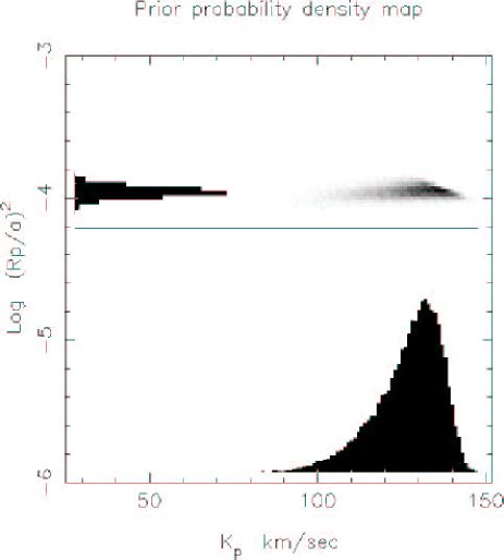
Figure 2: The greyscale shows the prior joint probability density function (PDF) for projected orbital velocity $K_{p}$ and the squared ratio $(R_{p}/a)^{2}$ of the planet radius to the orbit radius, based on the measured system parameters. Darker shades in the greyscale denote greater probabilities of the planet having the corresponding combination of $(R_{p}/a)^{2}$ and $K_{p}$. The one-dimensional projections of the PDF on to the two axes are shown as histograms. They show that the planet is most likely to have $K_{p}\simeq 135$ km s^-1 and $(R_{p}/a)^{2}\simeq 10^{-4}$. The horizontal line shows the value of $(R_{p}/a)^{2}$ for a 1 $R_{Jup}$ planet in the same orbit.

Orbital inclinations $i>80^{\circ}$ or so are ruled out by the absence of transits in high-precision photometry (?). The minimum inclination at which grazing transits occur is given by

$$\cos i_{min}=\frac{R_{\star}+R_{p}}{a}.$$ (5)

Low inclinations are also ruled out by the star’s chromospheric activity levels. The stellar radius and $v\sin i$ suggest an axial rotation period of 9 days. A $12\pm 2$ day period was estimated by Baliunas et al. (1997) based on four Ca ii H and K flux measurements and the period-activity-colour relation of Noyes et al. (1984). A more comprehensive study by ?, based on an additional 212 Ca ii H and K flux measurements in the 1996, 1997 and 1998 observing seasons shows the long-term average Ca ii H and K flux level to be almost identical to the original estimate by Baliunas et al. The rms scatter in the 30-day means is 4.7% of the long-term mean flux level. The 20% uncertainty in the 11.7-day period estimated from the long-term mean chromospheric flux is therefore dominated by the intrinsic scatter in of about 0.08 dex in the Noyes et al. (1984) calibration. Significantly faster axial rotation is needed to match the observed $v\sin i$ at orbital inclinations less than 60^∘, but is hard to reconcile with the observed chromospheric activity level. Henry et al. also point out that frequency analyses of the short-term variability in the 1996 and 1998 seasons yielded possible low-amplitude rotational modulation signals with periods of 11 and 19 days respectively, although both were classified as “weak”.

These rather loose constraints on $i$ require a Monte Carlo simulation to express our knowledge of the system parameters. For this we first generate a distribution of $\sin i$ values

$$\sin i=\frac{P_{CaII}.v\sin i}{2\pi R_{\star}}$$ (6)

computed from randomly-chosen values of the stellar rotation period, radius and $v\sin i$ and rejecting those combinations that yielded $\sin i>1$. We assume gaussian distributions for the log of the rotation period, the measured stellar mass and radius, and the stellar reflex velocity $K_{\star}$.

High inclinations are then eliminated by the observed absence of eclipses. Low $i$ are then given a reduced probability consistent with the measured $V_{rot}\sin{i}=9.5$ km s^-1 and estimate of its rotation period $P_{rot}\sim 12\pm 2$d, which together favour a relatively high $i$. The lower histogram in Fig. 2 shows the resulting probability distribution for $K_{p}$ (equivalent to $i$).

2.3 Rotational broadening

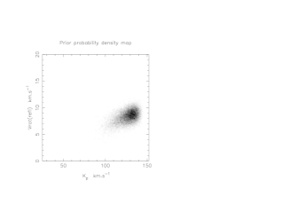
Figure 3: A Monte Carlo simulation shows how the apparent stellar equatorial rotation speed $v_{e,refl}$ in the starlight incident on the planet is expected to vary with the projected orbital velocity amplitude $K_{p}$. The system parameters are defined as in Section 2. The median rotational broadening of the reflected starlight is 8.4 km s^-1, somewhat less than the $v\sin i=9.5$ km s^-1 of the direct starlight.

The matched-filter analysis used to search for the reflected-light signal requires an a priori estimate of the rotational broadening of the spectral-line profiles in starlight reflected from the planet’s atmosphere.

The Earth-bound observer sees stellar aborption lines that are rotationally broadened by

$$v_{\star}\sin{i}=\frac{2\pi R_{\star}\sin{i}}{P_{rot,*}}=9.5\pm 0.8{\rm km~{}s}^{-1}\ .$$ (7)

We assume that the planet orbits in the same direction as the stellar rotation and that the orbital plane and stellar equator are coincident. The light received by the orbiting planet, and subsequently reflected toward an observer in any direction, then has a rotational broadening

$$v_{refl}=2\pi R_{\star}\left(\frac{1}{P_{rot,*}}-\frac{1}{P_{orb}}\right)\ .$$ (8)

The Monte Carlo simulation gives the resulting relationship between the broadening $v_{refl}$ of the reflected starlight and $K_{p}$, as shown in Fig. 3. The distribution of the predicted rotational broadening of the reflected starlight has a mean 8.3 km s^-1, $\sigma=1.1$ km s^-1, and median 8.4 km s^-1. The planet line widths are reduced at lower orbital inclinations, because the difference between the orbital and stellar rotation frequencies is reduced.

2.4 Albedo spectrum

The quantity that we observe is the ratio $f_{p}/f_{\star}$ of the spectral-line strengths in the planet’s light to those in the direct stellar spectrum as a function of wavelength:

$$\epsilon(\alpha,\lambda)\equiv\frac{f_{p}(\alpha,\lambda)}{f_{\star}(\lambda)}=p(\lambda)g(\alpha,\lambda)\frac{R_{p}^{2}}{a^{2}}=\epsilon_{0}(\lambda)g(\alpha,\lambda).$$ (9)

This depends on the fraction $(R_{p}/2a)^{2}$ of the star’s light intercepted by the planet, and the fraction of this light that is reflected towards the observer.

The monochromatic stellar flux illuminating the planet, orbiting at distance $a$, is

$$F_{\rm incident}(\lambda)=\frac{L_{\star}(\lambda)}{4\pi a^{2}}.$$ (10)

The geometric albedo $p(\lambda)$ is defined at $\alpha=0$

$$p(\lambda)=\frac{F_{\rm reflected}(0,\lambda)}{F_{\rm incident}(\lambda)}.$$ (11)

Here $F_{\rm reflected}(0,\lambda)=\pi I_{\rm reflected}(0,\lambda)$ is the disc-averaged flux of the starlight reflected from the planet directly back toward the star, also measured at the planet’s surface.

As the planet orbits the star, the observed flux varies with the star-planet-observer “phase angle” $\alpha$ as the product of the geometric albedo $p(\lambda)$ and a “phase function” $g(\alpha,\lambda)$ which is normalised to $g(0,\lambda)=1$.

The flux received from the planet at Earth, is therefore

$$f_{p}(\alpha,\lambda)=p(\lambda)g(\alpha,\lambda)F_{\rm incident}(\lambda)\frac{R_{p}^{2}}{D^{2}}.$$ (12)

Since the stellar flux received at Earth, a distance $D$ away, is

$$f_{\star}(\lambda)=\frac{L_{\star}(\lambda)}{4\pi D^{2}},$$ (13)

eq. 9 follows.

2.5 Phase function

Figure 4: Brightness variation of model planet with orbital phase assuming a Venus-like phase function (solid) or a Lambert sphere (dashed) for orbit inclinations $i=0,30,60,90^{\circ}$. In both cases, flux is measured relative to the value for illumination phase angle $\alpha=0$. The horizontal lines show the $i=0^{\circ}$ case, while $i=90^{\circ}$ gives the greatest amplitude.

The phase angle $\alpha$ depends on the orbital inclination $i$ and the orbital phase $\phi$ (measured from transit or inferior conjunction):

$$\cos\alpha=-\sin i.\cos 2\pi\phi.$$ (14)

The observations measure $\epsilon(\alpha,\lambda)$ over some range of orbital phases $\phi$ and hence phase angles $\alpha$. However, the signal-to-noise ratio and orbital phase coverage of the observations is not yet adequate to define the shape of the phase function. Accordingly, current practice is to adopt a specific phase function in order to express the results in terms of the planet/star flux ratio that would be seen at phase angle zero:

$$\epsilon_{0}(\lambda)=p(\lambda)\frac{R_{p}^{2}}{a^{2}}.$$ (15)

Since $a$ is tightly constrained through Kepler’s third law, given the period $P$ and the star mass $M_{\star}$, the measurements of $\epsilon_{0}(\lambda)$ measure the product $R_{p}\sqrt{p(\lambda)}$.

In this paper we adopt an empirical phase function similar to that of Venus and Jupiter. The expressions given in Appendix D.1 (eqs. 29 and and Eq. 31 for the phase function of a Lambert sphere and Venus respecively) yield the phase-dependent flux correction factors plotted in Fig. 4.

2.6 Planet radius and surface gravity

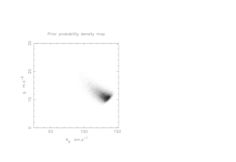
Figure 5: A Monte Carlo simulation shows how the gravitational acceleration $g$ at the planet’s surface is expected to vary with the projected orbital velocity amplitude $K_{p}$. The system parameters are defined as in Section 2. For comparison, $g_{Jup}=26.5$ m s^-2.

Because the surface gravity appears to play an important role in determining the height of the cloud deck and hence the albedo, we plot the relationship between $g$ and $K_{p}$ derived from the Monte Carlo simulations, in Fig. 5. The planet’s mass can be determined once the orbital inclination is known. Our a priori knowledge of the radius, however, comes only from structural models for close-orbiting giant planets.

In these models, the planet radius evolves with time and depends on the planet mass. For our purposes, theoretical mass-radius-age relations define a range of plausible radii at each possible value of the planet mass. The range of possible planet radii was computed specifically for $\upsilon$ And b by ?, allowing for uncertainties in the orbital inclination and hence the planet’s mass. Their radiative-convective gas giant models predict a radius between 1.2 and 1.7 $R_{\rm Jup}$ for $M_{p}=0.6M_{\rm Jup}$, to between 1.15 and 1.3 $R_{\rm Jup}$ for $M_{p}=1.15M_{\rm Jup}$.

When this mass-radius relation and its associated uncertainty are incorporated in the Monte Carlo model, we find that as the inclination decreases, the planet mass increases and the radius decreases. The lowest values of $g$ are therefore found when the orbit is, as is most probable, nearly edge-on to the line of sight (Fig. 5). The median predicted value, $g=11.6$ ms^-2, is close to the $\sim 10$ m s^-2 limit below which the Class V albedo models of ?) are applicable.

If Class V models apply, we can use them to estimate the planet’s brightness. Viewed fully illuminated, the reflected light from a planet with $(R_{p}/a)^{2}\simeq 10^{-4}$ and Class V albedo $p\simeq 0.42$ (cf. the Class V models of ?) is expected to be 24000 times fainter than the direct stellar spectrum in the visual band around 550 nm. At a phase angle of 60^∘, however, the reflected spectrum will be a factor two fainter than this (Fig.4).

3 Observations

Table 2: Journal of observations. The UTC mid-times and orbital phases are shown for the first and last groups of four spectra secured on each night of observation. The number of groups is given in the final column.

UTC start	Phase	UTC End	Phase	Number
				of groups
2001 Oct 09 22:27:51	0.296	2001 Oct 10 06:20:26	0.366	18
2001 Nov 06 19:43:04	0.335	2001 Nov 07 04:27:15	0.413	16
2001 Nov 07 19:25:48	0.549	2001 Nov 08 04:29:30	0.630	15

The strong dependence of the flux ratio on phase angle indicates that the best chance of a detection occurs shortly before and after superior conjunction. We observed $\upsilon$ And with the Utrecht Echelle Spectrograph on the 4.2-m William Herschel Telescope at the Roque de los Muchachos Observatory on La Palma, on the nights of 2000 Oct 10, Nov 6 and Nov 7. These nights were chosen to cover orbital phase ranges when the planet is on the far side of the star and well-illuminated, and its spectral signature is Doppler-shifted well clear of the wings of the stellar profile. The third night was partially affected by drifting cirrus cloud. Two further nights were also lost to cloud.

The detector was an array of two EEV CCDs, each with $2048\times 4096$ 13.5-$\mu$m pixels. The CCD was centred at 459.6 nm in order 124 of the 31 g mm^-1 echelle grating, giving complete wavelength coverage from 381.3 nm to 675.8 nm with minimal vignetting. The average pixel spacing was close to 1.6 km s^-1, and the full width at half maximum intensity of the thorium-argon arc calibration spectra was 3.5 pixels, giving an effective resolving power $R=53000$.

Table 2 lists the journal of observations for the three nights that contributed to the analysis presented in this paper. The stellar spectra were exposed for between 300 and 500 seconds, depending upon seeing, in order to expose the CCD to a peak count of 40000 ADU per pixel in the brightest parts of the image. A 450-s exposure yielded about $1.2\times 10^{6}$ electrons per pixel step in wavelength in the brightest orders in typical (1 arcsec) seeing after extraction. We achieve this with the help of an autoguider procedure, which improves efficiency in good seeing by trailing the stellar image up and down the slit by $\pm 2$ arcsec during the exposure to accumulate the maximum S:N per frame attainable without risk of saturation. Note that the 450-s exposure time compares favourably with the 53-s readout time for the dual EEV CCD in terms of observing efficiency – the fraction of the time spent collecting photons is above $90$ percent. Following extraction, the S:N in the continuum of the brightest orders is typically 1000 per pixel.

4 Spectrum extraction

One-dimensional spectra were extracted from the CCD frames using an automated pipeline reduction system built around the Starlink ECHOMOP and FIGARO packages. Nightly flat-field frames were summed from 50 to 100 frames taken at the start and end of each night, using an algorithm that identified and rejected cosmic rays and other non-repeatable defects by comparing successive frames. The nightly flat fields were then added to make a master flat-field for the entire year’s observations.

The initial tracing of the echelle orders on the CCD frames was performed manually on the spectrum of $\upsilon$ And itself, using exposures taken for this purpose without dithering the star up and down the slit. The automated extraction procedure then subtracted the bias from each frame, cropped the frame, determined the form and location of the stellar profile on each image relative to the trace, subtracted a linear fit to the scattered-light background across the spatial profile, and performed an optimal (profile and inverse variance-weighted) extraction (?; ?) of the orders across the full spatial extent of the object-plus-sky region. Flat-field balance factors were applied in the process. In all, 62 orders were extracted from each exposure. The blue CCD recorded orders 148 in the blue to 125 in the red, giving full spectral coverage from 380.7 to 461.0 nm with considerable wavelength overlap between adjacent orders. Orders 122 to 85 were recorded on the red CCD, covering the range 461.9 to 677.3 nm with good overlap. Orders 123 and 124 fell on the gap between the CCDs, but the loss in wavelength coverage was minimal.

5 Starlight-subtracted velocity-phase maps

The maximum expected flux of starlight scattered from $\upsilon$ And $b$ is, as we have seen, of order one part in 24000 of the flux received directly from $\upsilon$ And itself. In order to detect the planet signal, we first subtract the direct stellar component from the observed spectrum, leaving the planet signal embedded in the residual noise pattern.

To achieve this, we make a model of the direct starlight by aligning and summing all the spectra of the target from all nights of the run. The contribution of the planet to this summed spectrum is blurred by the planet’s orbital motion, so that to first order the planet’s spectrum is eliminated from the composite “template” spectrum. We then scale and distort this template spectrum to give the closest possible fit to each individual spectrum, using the spline-modulated Taylor-series method described in Appendix A.

When the aligned template is subtracted from each spectrum, we find that the residual spectrum contains a spatially fixed but temporally varying pattern of ripples, superimposed on random noise. The ripples are attributable to a combination of time-dependent changes in the detector’s sensitivity, thermal flexure in the spectrograph causing faint ghost reflections to shift slightly on the detector, and changes in the strength and velocity of telluric-line absorption features in some orders. We map the form of the ripple pattern using principal-component analysis, as described in Appendix B. After subtracting this map, we are left with a planet signal consisting of faint Doppler-shifted copies of thousands of stellar absorption lines, deeply buried in noise.

The positions and identifications of most of these thousands of lines are well-documented. We use the Vienna atomic-line database (VALD; ?) to compile a list of the wavelengths and relative central depths of the 3450 strongest lines falling in the observed wavelength range, for a model atmosphere appropriate to the spectral type and surface gravity of the star. We then use least-squares deconvolution (LSD; see Appendix C) to compute a composite profile which, when convolved with the line pattern, yields an optimal fit to the residual noise spectrum. This procedure is similar to cross-correlation in terms of the gain in S:N from the weighted summation of thousands of line profiles, but has the additional advantage of eliminating sidelobes caused by crosstalk with neighbouring lines.

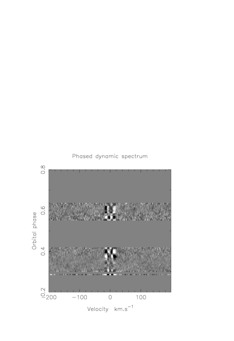
Figure 6: Velocity-phase map of deconvolved residual profiles derived from WHT spectra secured on 2000 Oct 09, Nov 06 and Nov 07. The line weights in the deconvolution were defined assuming a grey albedo spectrum. The greyscale runs from black at $-10^{-4}$ times the mean stellar continuum level, to white at $+10^{-4}$. The velocity scale is in the reference frame of the star.

The resulting devonvolved residual profiles are presented in greyscale form as a two-dimensional “velocity-phase” map in Fig. 6. This representation of the data shows a strong pattern of distortions in the residual stellar profiles within $\pm 20$ km s^-1 of the stellar velocity. These undulations in the deconvolved profiles appear to be caused by high-order mismatches in the spectrum subtraction procedure. Their amplitude is typically a few parts in $10^{4}$ of the average continuum level. They vary too rapidly during the night to be attributable to, e.g. stellar surface features causing time-dependent distortion of the stellar rotation profile. A more likely explanation is that the spatial profile produced by the telescope dithering procedure was not exactly repeatable from one frame to the next. Given that the slit image is slightly tilted with respect to the columns of the detector, this could give rise to small changes in the detailed shape of the line profile from one exposure to the next. Fortunately these ripples only affect a range of velocities at which the planet signature would in any case be indistinguishable from that of the star. We deliberately avoided observing between phases 0.45 and 0.55 for this reason.

Outside the residual line profile, we would expect to see a planet signature as a dark streak following a sinusoidal path that crosses the profile from positive to negative velocity at phase 0.5. No obvious planet signature is, however, visible in Fig. 6.

Figure 7: As for Fig. 6, with a simulated planet signature added at an orbital inclination of 80^∘. The model planet has a grey albedo spectrum with $p=0.42$ and a radius twice that of Jupiter, and its signature appears as a dark streak crossing from positive to negative velocity at phase 0.5.

We verified that a faint planetary signal is preserved through the analysis in the presence of realistic noise levels, by adding a simulated planetary signal to the observed spectra and performing the same sequence of operations described above. The simulation procedure simply consisted of shifting and scaling the spectrum of $\upsilon$ And according to the phase function, co-multiplying it by an appropriate geometric albedo spectrum, and adding it to the observed data.

To ensure a strong signal we assumed the planet to have a radius 2.0 times that of Jupiter, giving $(R_{p}/a)^{2}=2.57\times 10^{-4}$. Initially we used a wavelength-independent geometric albedo with $p=0.42$, which was chosen to match the continuum albedo of a Class V model unaffected by alkali-metal absorption. When viewed at zero phase angle, the planet-to-star flux ratio should thus be $\epsilon_{0}=f_{p}/f_{*}=1.08\times 10^{-4}$. We assumed an orbital inclination of 80^∘, giving an orbital velocity amplitude $K_{p}=137$ km s^-1 and a rotational broadening of the reflected starlight, $v_{e,refl}=8\pm 1$ km s^-1. We are therefore justified in using the spectrum of $\upsilon$ And itself, without any modification of the rotational broadening, to approximate the reflected-light spectrum.

The injected planet signal is clearly visible as a dark streak in Fig. 7. Given that no similar signal is easily seen in Fig 6, we can conclude that the planet in $\upsilon$ And is fainter than this one.

6 Extracting the planet signature

The form of the expected planet signature in the velocity-phase diagram can be represented accurately as a travelling Gaussian of characteristic width $\Delta v_{p}$ whose velocity varies sinusoidally around the orbit and whose strength is modulated according to the phase function $g(\alpha,\lambda)$ (see Appendix D.1). The value of $\Delta v_{p}$ is adjusted to match the expected rotational broadening of the reflected starlight. The amplitude $K_{p}$ of the velocity variation and the form of the phase function both depend on the orbital inclination $i$.

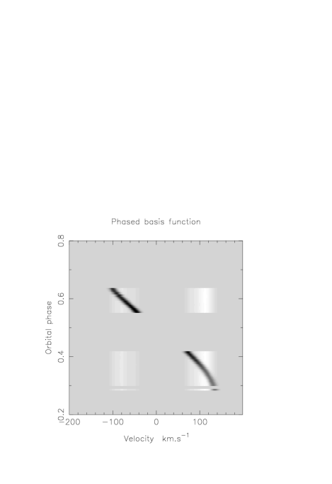
Figure 8: As for Fig. 6, but showing the matched filter function used to measure $(R_{p}/a)^{2}$ at $K_{p}=137$ km s^-1. The grey scale runs from -0.05 (black) to 0.01(white). Scaling this function to fit Fig. 6 (and others like it) yields the strength of the planet signal for a given value of $K_{p}$.

Fig. 8 shows the form of this model signal at an orbital inclination $i=80^{\circ}$. The weakening of the simulated planetary signature near quadrature (phases 0.25 and 0.75) is mostly the effect of the phase function. In some cases the signal may be further attenuated near quadrature by the way in which the templates are computed: since the planet signature is nearly stationary in this part of the orbit, some of the signal will be removed along with the stellar profile if many observations are made in this part of the orbit. The planet is detectable on a given night because its velocity changes while those of the stellar lines do not. Thus observations at quadrature are less helpful. In the present dataset, few observations were made near quadrature so this problem does not arise.

The travelling gaussian in this image has nonetheless been modified to give an even closer match to the observed planet signal, by subtracting its own flux-weighted average. This procedure mimics the attenuation of the planet signal that occurs when the template spectrum is subtracted from the individual spectra. The main effect of the template subtraction is to produce the bright vertical zones seen centred at $v\simeq-70$ km s^-1 and $v\simeq+100$ km s^-1 in Fig. 8.

Figure 9: The upper panel shows the optimal scaling factor $(R_{p}/a)^{2}$ plotted against orbital velocity amplitude $K_{p}$, assuming a grey albedo spectrum with $p=0.42$. The lower panel shows the associated reduction in $\chi^{2}$ measured relative to the fit obtained in the absence of any planet signal, i.e. for $(R_{p}/a)^{2}=0$. Note that only positive values of $(R_{p}/a)^{2}$ are physically plausible, so the middle peak in the $\Delta\chi^{2}$ plot is unambiguously a noise feature.

Figure 10: Relative probability map of model parameters $K_{p}$ and $\log(\epsilon_{0}/p)=\log(R_{p}/a)^{2}$, derived from the WHT/UES observations of $\upsilon$ And, assuming a grey albedo spectrum with $p=0.42$. The greyscale denotes the probability relative to the best-fit model, increasing from 0 for white to 1 for black. From bottom to top, the contours show the 1, 2, 3 and 4$\sigma$ upper limits limits on the signal strength derived from the bootstrap trials The uppermost contour, for example, represents the value of $\log(R_{p}/a)^{2}$ that was only exceeded in 3 of 3000 bootstrap trials at each $K_{p}$. It gives a robust empirical estimate of the upper limit on the planet radius allowed by the data for the grey albedo model with $p=0.42$ assumed here.

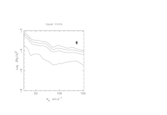
Figure 11: Relative probability map of model parameters $K_{p}$ and $\log(\epsilon_{0}/p)=\log(R_{p}/a)^{2}$ for a simulated planet signature with grey albedo $p=0.42$, $K_{p}=137$ km s^-1, and $R_{p}=2R_{Jup}$. The greyscale and contours are defined as in Fig. 10. The synthetic planet signature is detected well above the 4$\sigma$ upper limit on the strength of noise features in the absence of a planet signal.

7 Probability maps for $K_{p}$ and $R_{p}/a$

We use a sequence of such models for different values of $K_{p}$ as matched filters to measure the strengths and velocity amplitudes of possible faint planet signals of the expected form in the velocity-phase maps. At each of a sequence of trial values of $K_{p}$ we construct a model $H_{ij}(K_{p})$ like that shown in Fig. 8 and scale it to give an optimal fit to the residual velocity-phase map $D_{ij}$ using the methods presented in Appendix D. For an assumed albedo spectrum $p(\lambda)$ and orbital velocity amplitude $K_{p}$, the fit of the matched filter to the data measures $(R_{p}/a)^{2}$.

The badness-of-fit statistic $\chi^{2}$ gives a relative measure of the probability that any signal detected could have arisen by chance, and is quantified by

$$\chi^{2}=\sum_{i,j}\frac{(D_{ij}-(R_{p}/a)^{2}H_{ij}(K_{p}))^{2}}{\sigma^{2}_{ij}}.$$ (16)

Here $\sigma^{2}_{ij}$ is the variance associated with $D_{ij}$, computed from the photon statistics of the original image and propagated through the deconvolution (see Appendix C).

In Fig. 9 we plot the optimum scale factor and the associated improvement in $\chi^{2}$ measured relative to the no-planet model. For a noise-dominated signal, the estimated value of $(R_{p}/a)^{2}$ will be negative about as often as it is positive, and Fig. 9 bears this out. Three candidate peaks are seen in the lower panel, of which only the first and the third correspond to positive (and therefore physically plausible) reflected-light fluxes. The third (positive) peak gives the greatest improvement in $\chi^{2}$ and is therefore the most probable, but only by a narrow margin.

The relative probabilities of the fits to the data for different values of the free parameters $R_{p}/a$ and $K_{p}$, given by

$$P(K_{p},(R_{p}/a)^{2})=\exp(-\chi^{2}/2),$$ (17)

are shown in Fig. 10. To make this figure, a planet signal pattern as in Fig. 8 was computed for many different $K_{p}$, and each one was scaled by $(R_{p}/a)^{2}$ to fit the residuals in Fig 6. The greyscale is defined such that white represents the probability of a model fit where no planet signal is present, while black represents the most probable solution in the map. The curves give 1, 2, 3 and 4$\sigma$ detection thresholds derived from the bootstrap procedure discussed below.

To set an upper limit on the strength of the planet signal, or to assess the likelihood that a candidate detection is spurious, we need to compute the probability of obtaining such an improvement in $\chi^{2}$ by chance alone. In principle this could be done using the $\chi^{2}$ distribution for 2 degrees of freedom. In practice, however, the distribution of pixel values in the deconvolved difference profiles has extended non-gaussian tails that demand a more cautious approach.

Rather than relying solely on formal variances derived from photon statistics, we use a “bootstrap” procedure to construct empirical distributions for confidence testing, using the data themselves. The bootstrap procedure, detailed in Appendix E, interchanges at random the order of the nights, and rearranges at random the order of spectra in each night, thereby scrambling planet signals while retaining the same pattern of systematic errors, phase sampling, and statistical noise as in the actual data.

The 68.4%, 95.4%,99.0% and 99.9% percentage points of the resulting bootstrap distribution of $(R_{p}/a)^{2}$ at each $K_{p}$ are shown as contours in Fig. 10 and Fig. 11. From bottom to top, the contours give the 1, 2, 3, and 4$\sigma$ bootstrap upper limits on the strength of the planet signal. They represent the signal strengths at which spurious detections occur with 32, 5, 1, and 0.1% false alarm probability respectively, for each fixed value of $K_{p}$.

Table 3: Upper limits on planet dimensions for various albedo models. The upper limits are quoted for an assumed $K_{p}\simeq 135$ km s^-1, near the peak of the prior probability distribution for $K_{p}$. Note that the results for the grey albedo model are quoted for unit geometric albedo. To obtain the radii for grey models with other values of $p$, the radii in Column 4 should be divided by $\sqrt{p}$.

Albedo	False-alarm	$(R_{p}/a)^{2}$	$R_{p}/R_{Jup}$
model	probability
Grey	0.1%	0.58E-04	0.98
($p=1.00$)	1.0%	0.45E-04	0.86
	4.6%	0.34E-04	0.75
Class V	0.1%	1.42E-04	1.53
	1.0%	1.11E-04	1.35
	4.6%	0.87E-04	1.19
Class IV	0.1%	3.02E-04	2.23
(Isolated)	1.0%	2.20E-04	1.90
	4.6%	1.68E-04	1.66

7.1 Grey albedo model

At the most probable values around $K_{p}\simeq 135$ km s^-1, the grey albedo model yields a 0.1% bootstrap upper limit on the planet/star flux ratio $\epsilon_{0}<5.84\times 10^{-5}$. Adopting a grey albedo model with unit geometric albedo, we find that the 0.1%, 1.0% and 4.6% upper limits on $\epsilon_{0}$ at this velocity correspond to upper limits on the planet radius as listed in Table 3. If the orbital inclination is lower, the planet radius is less strongly constrained.

Table 4: Orbital velocity amplitude, signal strength, planet radius, $\Delta\chi^{2}$ and false-alarm probabilities (FAP) for possible planet signals. The FAP is computed for two different priors. The first prior is uniform in $K_{p}$ from 44 to 152 km s^-1. The second weights $K_{p}$ in proportion to the prior probability based on Caii H & K emission and $v\sin i$ constraints and the absence of eclipses. In the latter case, the false-alarm probability for the $K_{p}=132$ km s^-1 candidate is found to be between 9 and 10 percent.

Albedo	$K_{p}$	$(R_{p}/a)^{2}$	$R_{p}/R_{Jup}$	$\Delta\chi^{2}$	FAP	FAP
model	(km s-1)	($\times 10^{-4}$)			(uniform weight)	($K_{p}$ prior)
Grey	54	$0.87\pm 0.25$	$1.20\pm 0.17$	11.93	0.324	0.975
($p=1.00$)	132	$0.39\pm 0.11$	$0.80\pm 0.11$	13.61	0.259	0.094
Class V	50	$2.08\pm 0.64$	$1.85\pm 0.29$	10.39	0.423	0.983
	132	$1.09\pm 0.28$	$1.34\pm 0.17$	14.61	0.240	0.087
Class IV	49	$3.39\pm 1.31$	$2.36\pm 0.47$	6.66	0.534	0.995
	132	$1.73\pm 0.52$	$1.68\pm 0.25$	10.78	0.285	0.099

Two possible planet signals of comparable likelihood are seen. Their properties are listed in Table 4. The stronger, at $K_{p}\simeq 132$ km s^-1 ($i\simeq 80^{\circ}$), yields an improvement $\Delta\chi^{2}=13.61$ over the model fit obtained assuming no planet signal is present. If this feature represents a genuine planet signal, its velocity amplitude $K_{p}=132$ km s^-1 implies a planet mass $M_{p}=0.74M_{Jup}$ and (for $p=0.42$) a planet radius $R_{p}=1.24\pm 0.17R_{Jup}$. The weaker candidate has $K_{p}\simeq 54$ km s^-1 ($i=22^{\circ}$) and $\Delta\chi^{2}=11.86$, and gives a larger planet radius.

We used the bootstrap simulations to determine the probability that a spurious detection with $\Delta\chi^{2}>13.61$ could be produced by a chance alignment of noise features in the absence of a genuine planet signal. It is important to note that the location of the “blob” between the 2$\sigma$ and 3$\sigma$ bootstrap contours in Fig. 10 does not imply a false-alarm probability of $\sim 3$%. These contours give the false-alarm probability only if the value of $K_{p}$ is known in advance, which is not the case here. The true false-alarm probability is greater, being the frequency with which spurious peaks at any plausible value of $K_{p}$ can exceed the $\Delta\chi^{2}$ of the candidate. If we assume that all values of $K_{p}$ are equally likely in the range 44 km s${}^{-1}<K_{p}<152$ km s^-1 over which our phase coverage allows signals to be detected, the false-alarm probability is found to be 26% via the method described in Appendix E.

In practice, however, we are more likely to be fooled into believing that a candidate detection near the peak of the a priori probability distribution for $K_{p}$ is genuine, than would be the case if the candidate appeared at a velocity that was physically implausible given our existing knowledge of the system parameters. We can therefore refine the search range in $K_{p}$ using our knowledge of the a priori probability distribution for $K_{p}$, via the method presented in Appendix E. The last two columns of Table 4 show clearly that, while the unweighted false alarm probabilities for the features near $K_{p}=132$ and $K_{p}=54$ km s^-1 are comparable, the latter is almost certainly spurious. The false-alarm probability for the $K_{p}=132$ km s^-1 feature drops to 9.4% when prior knowledge of $K_{p}$ is accounted for, while that for the 54 km s^-1 feature approaches unity.

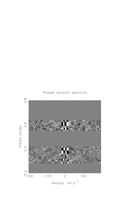
Figure 12: As for Fig. 6, showing the time-series of deconvolved profiles derived from the original observations assuming the albedo spectrum to be that of a Class V roaster.

Figure 13: As for Fig.9, showing the optimal scaling factor $(R_{p}/a)^{2}$ and the associated improvement in $\chi^{2}$ plotted against orbital velocity amplitude $K_{p}$, assuming a Class V albedo spectrum.

Figure 14: Relative probability map of model parameters $K_{p}$ and $\log(\epsilon_{0}/p)=\log(R_{p}/a)^{2}$, derived from the WHT/UES observations of $\upsilon$ And, assuming the albedo spectrum to be that of a Class V roaster. The greyscale and contours are defined as in Fig. 10.

For comparison, we show in Fig 11 a probability map derived by subtracting Fig. 6 from Fig. 7 to isolate the injected planet signal, then performing the matched-filter analysis. The injected planet is clearly detected as a compact, dark feature with its correct amplitude $\log(R_{p}/a)^{2}=2.57\times 10^{-4}$ and orbital velocity amplitude velocity $K_{p}=137$ km s^-1. This most probable combination of orbital velocity and planet radius yields an improvement $\Delta\chi^{2}=98.6$ with respect to the value obtained assuming no planet is present (i.e. $R_{p}=0$). This is far greater than the greatest $\Delta\chi^{2}=55.3$ produced at any value of $K_{p}$ in any of the bootstrap trials. The false-alarm probability for this simulated signal is substantially less than one part in 3000, and the “detection” is secure.

We note that the calibration of the $(R_{p}/a)^{2}$ scale in Fig. 10 depends on the value $p=0.42$ assumed for the geometric albedo. In the next sections, we explore the relative ability of non-grey albedo models to fit the data.

7.2 Class V roaster model

The “Class V roaster” is the most highly reflective of the models computed by ?. This model is characteristic of planets with $T_{eff}\geq 1500$ K and/or surface gravities lower than $\sim 10$ m s^-2, and has a silicate cloud deck located high enough in the atmosphere that the overlying column density of gaseous alkali metals is low, allowing a substantial fraction of incoming photons at most optical wavelengths to be scattered back into space. There remains, however, a substantial absorption feature around the Na I D lines, as shown in Fig. 1. If $\upsilon$ And b has a mass and radius close to the values at the peak of the prior probability distribution, its surface gravity is close to the critical limit (Fig. 5).

We carried out the deconvolution using the same line list as for the grey model, but with the line strengths attenuated using the Class V albedo spectrum (see Appendix C). We back-projected the resulting time series of deconvolved profiles (Fig. 12) as described above. We calibrated the signal strength as described in Appendix D.4, by injecting an artificial planet signature consisting of the spectrum of $\upsilon$ And, attenuated by the Class V albedo spectrum and scaled to the signal strength expected for a planet with $R_{p}=2R_{jup}$. For the observations we used $\Delta v_{p}=8$ km s^-1 which again yielded the best fit, with scale factors and improvements in $\chi^{2}$ as plotted in Fig. 13. The probability map for the observed signals is shown in Fig. 14.

The form of the Class V probability map is similar to that encountered for the grey albedo spectrum. The resulting upper limits on the planet radius are listed in Table 3. The local probability maxima near $K_{p}=52$ and 132 km s^-1 are also present with this albedo model. As in the grey case, the feature at $K_{p}=132$ is the most probable, this time by a slightly wider margin. Their signal strengths and false-alarm probabilities are given in Table 4.

Figure 15: As for Fig. 6, showing the time-series of deconvolved profiles derived from the original observations assuming the albedo spectrum to be that of an “isolated” Class IV roaster.

Figure 16: As for Fig.9, showing the optimal scaling factor $(R_{p}/a)^{2}$ and the associated improvement in $\chi^{2}$ plotted against orbital velocity amplitude $K_{p}$, assuming an isolated Class IV albedo spectrum.

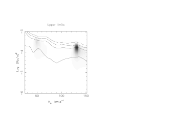
Figure 17: Relative probability map of model parameters $K_{p}$ and $\log(\epsilon_{0}/p)=\log(R_{p}/a)^{2}$, derived from the WHT/UES observations of $\upsilon$ And, assuming the albedo spectrum to be that of an “isolated” Class IV roaster. The greyscale and contours are defined as in Fig. 10.

7.3 Isolated Class IV model

The Class IV roaster models of ? have a more deeply-buried cloud deck than the Class V models. The resonance lines of Na I and KI are strongly saturated, with broad wings due to collisions with H₂ extending over much of the optical spectrum (Fig. 1).

We used the procedures described above to deconvolve and back-project the data assuming an “isolated” Class IV spectrum. Although this model does not take full account of the effects of irradiation of the atmospheric temperature-pressure structure, it is a useful compromise between the Class V models and the very low albedos found with irradiated Class IV models. The resulting time-series of deconvolved spectra (Fig. 15) is noisier than the Class V and grey-albedo versions, because lines redward of 500 nm contribute little to the deconvolution. Consequently, the derived upper limits on the planet radius (Table 3) are higher than for the Class V albedo model.

The plots of $(R_{p}/a)^{2}$ and $\Delta\chi^{2}$ versus $K_{p}$ show the same mix of positive and negative signal amplitudes encountered with the grey and class V spectral models. The back-projected probability map (Fig.17) nonetheless shows the $K_{p}=132$ km s^-1 probability maximum to be present and again stronger than the 49 km/sec feature. The fit to the data is, however, poorer than in the grey and Class V cases, giving an improvement of only $\Delta\chi^{2}=10.8$ over the no-planet hypothesis and a planetary radius $R_{p}=1.68\pm 0.25R_{Jup}$ (Table 4). This is 25% larger than the radius estimated with the Class V albedo model. The bootstrap test gives a false-alarm probability of 10%.

This relatively large radius and poor fit appear to arise from a mismatch between the wavelength dependence of the putative planet signal and the Class IV model. We tested this notion by deconvolving and back-projecting a synthetic Class V model using the Class IV line weights and flux calibration. The radius of the planet was over-estimated by 27% in this experiment. This occurs because the least-squares deconvolution is attempting to fit a set of lines at all wavelengths, with a deconvolution mask in which the lines at red wavelengths are too weak to fit the data properly. The best compromise is achieved (in the least-squares sense) by over-estimating the depth of the deconvolved profile in order to boost the strengths of the weakened lines.

We conclude that the faint signals that contribute to the $K_{p}=132$ km s^-1 feature are distributed in wavelength in a way that resembles more closely a grey or a Class V spectrum than a strongly-absorbed Class IV spectrum in which only blue light is present.

7.4 Plausibility of candidate signals

Comparison of Figs.10, 14 and 17 with the joint prior probability distribution in Fig. 2 shows that the feature near $K_{p}=50$ km s^-1 yields a value of $(R_{p}/a)^{2}$ that is considerably greater than the radius predicted by ?. The feature at $K_{p}=132\pm 3$ km s^-1, however, has $\epsilon_{0}=4.6\times 10^{-5}$. A plausible geometric albedo $p=0.42$ then gives $(R_{p}/a)^{2}=(1.09\pm 0.30)\times 10^{-4}$, which places it very close to the peak of the joint prior probability distribution.

We probed the rotational broadening of the candidate features by performing a series of backprojections using values of the gaussian width parameter in the range $6.4<\Delta v_{p}<10$ km s^-1, corresponding to $0<v_{e,refl}<11.3$ km s^-1. The feature at 132 km s^-1 yields the greatest improvement in $\chi^{2}$ when $\Delta v_{p}=8\pm 1$ km s^-1, or $v_{e,refl}=7.0\pm 2$ km s^-1. The 52 km s^-1 feature, however, grows less significant as $v_{e,refl}$ is decreased to the (retrograde) 5 km s^-1 or so expected at the corresponding orbital inclination. The rotational broadening of the 132 km s^-1 feature is therefore consistent with the value predicted in Fig. 3.

We explored the region of parameter space around both features, by carrying out back-projections on a grid of orbital periods and epochs of zero phase around the values given in Table 1, taking the epoch of transit to be near the middle of the data train to ensure that the period and epoch were uncorrelated. The local minimum in $\chi^{2}$ was found to be centred at $K_{p}=133\pm 3$ km s^-1, $P=4.621\pm 0.005$ d, and $T_{0}=2451853.770\pm 0.025$. The radial-velocity ephemeris gives $P=4.61707\pm 0.00003$ d and $T_{0}=2451853.777\pm 0.012$, well within the 1$\sigma$ error bars derived from the back-projection. The 52 km s^-1 feature, on the other hand, is part of a more extended structure whose peak is located at $K_{p}=67\pm 3$ km s^-1, $P=4.651\pm 0.006$ d, and $T_{0}=2451853.81\pm 0.02$. This bears little relation to the radial-velocity solution, suggesting a spurious origin.

We conclude that the candidate feature at $K_{p}=132$ km s^-1 corresponds to a local minimum of $\chi^{2}$ with respect to the parameters of interest, whose rotational broadening, phasing and velocity amplitude are consistent with those expected of a reflected-light signature from a planet whose orbital inclination is near the most probable value. We cannot easily dismiss this feature as being merely an extension of a larger, spurious noise-induced structure.

8 Conclusions

The observations of $\upsilon$ And presented here rule out radii for the innermost planet greater than $R_{p}>0.98R_{jup}/\sqrt{p}$ with 0.1% false-alarm probability if a grey albedo spectrum is assumed. We derive upper limits also with 0.1% false-alarm probability on the planet’s radius of 1.53 $R_{jup}$ assuming the albedo spectrum of a Class V roaster (low gravity, high cloud deck, ?), or 2.23 $R_{jup}$ for an isolated Class IV model with saturated Na I D absorption from 550 nm to the red limit of our spectra. We cannot, however, rule out the possibility that the planet has an albedo spectrum as bright as a Class V roaster (?) if its radius is comparable to that of HD 209458 b. The evidence for a reflected-light signature in the observations reported here, at a projected orbital velocity amplitude $K_{p}=132\pm 3$ km s^-1, is marginal but encouraging. If the orbital inclination is as close to edge-on as we infer from previously-measured system parameters, the mass and radius of the planet yield a surface gravity low enough for a Class V atmosphere to be plausible. If future observations confirm this signal, it gives a radius $R_{p}=1.34\pm 0.17R_{Jup}$ if a Class V spectrum is assumed. This is comparable to the radius of HD 209458 b inferred from HST transit photometry (?).

We have explored the spectral properties of the candidate detection via the relative probabilities of the fits to the data. The Class V roaster model gives a slightly better fit to the data than a grey albedo model. Both yield planet radii and orbital velocity amplitudes close to the peak of the prior probablility density function. The isolated Class IV albedo model gives a significantly poorer fit to the data.

While the possible detection discussed here gives believable physical properties for the innermost planet, it remains too marginal for us to claim a bona fide detection of reflected starlight. Our bootstrap analysis suggests a 7% to 10% likelihood that the feature could be a spurious noise feature. There is clearly a strong case for a deeper reflected-light search to be made in the $\upsilon$ And system.

Appendix A Removal of direct starlight

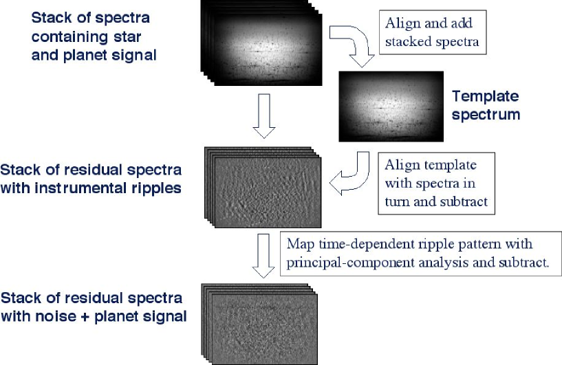
Figure 18: Schematic illustration of the main steps in the construction and subtraction of the template spectrum, and the subsequent fixed-pattern noise removal.

In this appendix we describe the procedure we use to subtract the stellar spectrum without introducing substantial noise and also without subtracting the planet signal. The intrinsic spectrum of the star was modelled as the co-aligned sum of all the spectra of $\upsilon$ And secured during the run.

We began by removing cosmic-ray hits from the individual frames. Within each night’s data, each frame was divided by its predecessor and the result was median smoothed with a box covering 21 pixels in the dispersion direction and 5 adjacent orders. This smoothed frame was used to scale the predecessor frame, which was then subtracted from the frame under consideration. The difference frame was divided by the square root of the frame under consideration, to yield deviates in units of the local Poissonian noise amplitude. All pixels whose deviates were more than 7 sigma in excess of their counterparts in the scaled predecessor frame were assumed to be cosmic ray hits. Their values were replaced with values taken from the corresponding pixels in the scaled predecessor frame. The result was re-scaled and added to the scaled predecessor frame to restore the original frame with all major cosmic-ray hits removed. The cleaned frames were then shifted to co-align the stellar absorption lines to the nearest integer pixel. Finally the cleaned frames were summed to make the template frame (step 1 in Fig. 18).

The individual cleaned frames were co-added in groups of four for the next stage in the procedure, which involved scaling, shifting and blurring (or sharpening) the template frame prior to subtraction from each group. The first and second derivatives of the template frame were computed from the template values $t_{j}$ in each order as a function of pixel number $x_{j}$ in the dispersion direction:

$$t^{\prime}_{j}=\frac{t_{j+1}-t_{j-1}}{x_{j+1}-x_{j-1}}$$ (18)

and

$$t^{\prime\prime}_{j}=2\frac{(t_{j+1}-t_{j})/(x_{j+1}-x_{j})-(t_{j}-t_{j-1})/(x_{j}-x_{j-1})}{x_{j+1}-x_{j-1}}.$$ (19)

The third and fourth derivatives were computed by applying the same operations to $\mbox{\boldmath${t}$}^{\prime\prime}$, for use in correcting frame-to-frame changes in the higher moments of the PSF and seeing profile.

The vector ${f}$ of all observed spectrum values within each extracted echelle order was then modelled by scaling the template ${t}$ along each order, the scale factors varying as a function of position ${x}$ approximated by a 34-knot least-squares spline. The use of such a high-order spline was demanded by vignetting near the edges of each order, which produced an abrupt and time-variable change in the slope of the stellar continuum towards the end of each order. The derivative frames were scaled in a similar fashion, using 6-knot splines to define the scale factors. An additional 6-knot spline was added to the fit to provide a smooth background correction for any inconsistencies in the scattered-light subtraction during the extraction process. The scaled, aligned, distorted template spectrum thus had the form

$$g_{j}=\alpha_{j}t_{j}+\beta_{j}t^{\prime}_{j}+\gamma_{j}t^{\prime\prime}_{j}+\delta_{j}t^{\prime\prime\prime}_{j}+\epsilon_{j}t^{\prime\prime\prime\prime}_{j}+\eta_{j}$$ (20)

where $\alpha_{j}$ is the value at $x_{j}$ of the 34-knot spline and $\beta_{j}$, $\gamma_{j}$, $\delta_{j}$, $\epsilon_{j}$ and $\eta_{j}$ are the values of the corresponding 6-knot splines used to scale the derivatives and correct the background. The knot values for the various splines were determined by the method of least squares using singular-value decomposition to ensure that spurious fluctuations were suppressed in those parts of the spectrum where few lines were present.

When the planet velocity is sufficient to shift the absorption lines in the reflected starlight well away from those in the direct starlight, then the residual spectrum $\mbox{\boldmath${r}$}=\mbox{\boldmath${f}$}-\mbox{\boldmath${g}$}$ is expected to retain the reflected starlight signal, Doppler shifted and deeply buried in Poissonian noise, once step 2 in Fig. 18 is complete.

Appendix B Residual fixed-pattern noise

In this appendix we describe the principal-component analysis method used to correct the spatially fixed but time-dependent ripples found in the residual spectra following subtraction of the template.

Typically the grouped spectra contained $4\times 10^{6}$ or more photons per pixel over most of the recorded spectrum. The scatter of the pixel values in the residual spectrum was compared with expectations from photon statistics, by dividing each grouped spectrum through by the square root of its computed variance. The distribution of the pixel deviates calculated over the 62 orders used for the deconvolution (see Appendix C below) was found typically to contain a few hundred extreme outliers, mostly caused by systematic errors in the polynomial fits in half a dozen regions affected by defects on the CCD. Despite clipping at $\pm 4$ times the expected local root-mean-square (rms) photon noise amplitude, we found that the distribution of the remaining values was Gaussian with an rms error between 1.4 and 1.6 times the expected value. We found a significant correlation between pixel values in successive difference frames, indicating that some fixed-pattern noise sources had not been eliminated fully by the template alignment and subtraction. The residuals were correlated over a few hours in time. The residuals in pairs of frames taken several hours apart or on different nights were also found to be correlated, though in some instances the slope of the correlation was reduced or even reversed. The fixed-pattern noise is visible as ripples in the example frame shown following step 2 in Fig. 18.

We mapped these spatially fixed but time-varying patterns in the difference spectra using principal-component analysis (PCA). We start with a set of $M$ spectra, each of length $N$ pixels. The $i$th spectrum thus has elements $\mbox{\boldmath${s}$}_{i}=\{s_{i1},s_{i2},\ldots,s_{iN}\}$ and associated variances $\mbox{\boldmath${\sigma^{2}}$}_{i}=\{\sigma^{2}_{i1},\sigma^{2}_{i2},\ldots,\sigma^{2}_{iN}\}$. The spatial correlation matrix of the time variations in the individual spectral bins of this set of spectra is a real symmetric matrix of dimensions $N\times N$, whose elements are given by:

$$H_{jk}=\sum_{i=1}^{M}\frac{(s_{ij}-\hat{s}_{j})(s_{ik}-\hat{s}_{k})}{\sigma_{ij}\sigma_{ik}}.$$

Note that we subtract the inverse variance weighted mean spectrum $\hat{s}$ before computing the correlation matrix. The $j$th spectral bin of $\hat{s}$ is given by:

$$\hat{s}_{j}=\frac{\sum_{i=1}^{M}s_{ij}/\sigma^{2}_{ij}}{\sum_{i=1}^{M}1/\sigma^{2}_{ij}}.$$

The principal components are those eigenvectors of the correlation matrix accounting for the largest fraction of the variance, and in our implementation are computed using Jacobi’s method (?). To keep computing time down, we processed the spectra in segments of length 100 pixels.

We found that most of the unwanted additional variance was contained in the first two principal components, indicating that two independent sources of fixed-pattern noise were present. The first principal component contained a spatially fixed but temporally-varying pattern of ripples affecting all orders, which is probably attributable to a slow drift in the sensitivity pattern of the flat field and/or thermal flexure in the spectograph. The second principal component consisted mainly of imperfectly-subtracted telluric absorption features in some orders. We computed the contributions of these two fixed-pattern noise sources to each exposure and subtracted them from the difference frames. This effectively removed the correlation between successive frames, and reduced the RMS scatter in the pixel values to within $\pm 10$% of the value expected from photon statistics alone (step 3 in Fig. 18). The planet signature should not be affected by this procedure any more than it is affected by the template subtraction because, unlike the fixed-pattern noise, it is smeared out by orbital motion.

Appendix C Least-squares deconvolution

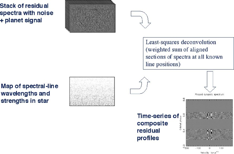
Figure 19: Schematic illustration of the main steps in the least-squares deconvolution of a time-series of spectra.

We extracted the reflected-light signature from the difference frames using the method of weighted least-squares deconvolution (LSD) described by ?. This method, shown schematically in Fig. 19) entails taking a list of lines with relative strengths appropriate to the type of star concerned, and computing via the method of least squares a “mean” line profile which, when convolved with the line pattern, gives an optimal match to the observed spectrum. The deconvolved profile thus incorporates an average broadening function that is representative of all the lines recorded in the spectrum. Applied to the residual spectrum from which the direct stellar signal has been removed, LSD is an effective way of measuring the average line profile of the faint reflected-light signature of the planet, because the reflected light should should have the same pattern of absorption-line positions and strengths as the stellar spectrum.

In terms of signal improvement, LSD is analogous to aligning and averaging (with appropriate weighting factors for line strength and local continuum signal strength on the recorded frame) the profiles of all the individual photospheric absorption lines recorded on each echellogram and included in the line list. As each individual spectral line appears in at least two adjacent echelle orders, we have 7700 images of the 3450 spectral lines listed in the observed wavelength range. If all lines were of equal strength and the continuum signal were constant over the whole frame, the signal-to-noise deconvolved profile would be proportional to the square root of the number of line images used, i.e. nearly 70 times greater than the signal-to-noise ratio of a single line in the original spectrum. In practice, the recorded continuum is not uniform and the lines have a wide variety of depths. Even so, the signal-to-noise ratio of the deconvolved profile is found to be some 30 times greater than that of a single line in the best-exposed parts of the original spectrum. The least-squares fitting procedure has the additional advantage that neighbouring, blended lines are treated simultaneously, thereby eliminating the sidelobes that would be produced by a simpler shift-and-add procedure.

We divide the observed residual spectrum by the continuum fit to the original spectrum, to obtain a normalised residual spectrum ${r}$ expressed in units of the continuum level of the original spectrum. We modify the variances associated with the elements of ${r}$ accordingly. We treat ${r}$ as the convolution of a “mean” line profile $\mbox{\boldmath${z}$}(v)$ with a set of weighted delta functions at the wavelengths of a comprehensive list of spectral lines. The profile ${z}$ is defined on a linear velocity scale, with a velocity increment $\Delta v=3$ km s^-1 per bin, which is close to the average velocity increment per pixel in the extracted spectra. The elements $A_{jk}$ of the convolution matrix $A$ are computed by summing, over all spectral lines $\ell$, the fractional contribution of the element of the deconvolved profile at velocity $v_{k}$ to the data pixel at wavelength $\lambda_{j}$ when the centre of the deconvolved profile is shifted to the wavelength $\lambda_{\ell}$ of each line in turn. Hence

$$A_{jk}=\sum_{\ell}w_{\ell}\Lambda[(v_{k}-c(\lambda_{j}/\lambda_{\ell}-1))/\Delta v].$$ (21)

The triangular function $\Lambda$ has the form $\Lambda(x)=1+x$ for $-1<x\leq 0$, $\Lambda(x)=1-x$ for $0<x<1$, and is zero everywhere else. The line weights $w_{\ell}$, incorporated in the convolution matrix ${A}$, are proportional to the central depths of the lines as computed from a Kurucz model atmosphere for the appropriate spectral type. After some experimentation we found that a line list computed for a G2 spectral type with solar abundances gave the best results. The use of a cooler template gives a better fit to the line depths than an earlier spectral type, presumably because of the star’s above-solar metallicity.

Because the form of the geometric albedo spectrum of $\upsilon$ And b is unknown, we investigated the effects of both grey (i.e. wavelength-independent) and non-grey geometric albedo spectra. The non-grey models we employed were the Class V and “isolated” Class IV models of ? (Fig. 1). The theoretical albedo spectra provided an additional weighting factor in the deconvolution linelist, allowing us to place limits on the planet’s radius for any assumed albedo model, and to assess the relative goodness-of-fit to the data for different atmospheric models.

The deconvolved profile $\mbox{\boldmath${z}$}(v)$ has the form of a line profile normalized to unit continuum intensity, but from which the continuum has been subtracted. Determination of $\mbox{\boldmath${z}$}(v)$ via least squares entails minimizing the magnitude of the misfit vector $|\mbox{\boldmath${r}$}-\mbox{\boldmath${A}$}\cdot\mbox{\boldmath${z}$}|$,

$$\chi^{2}=(\mbox{\boldmath${r}$}-\mbox{\boldmath${A}$}\cdot\mbox{\boldmath${z}$})^{T}\cdot\mbox{\boldmath${V}$}\cdot(\mbox{\boldmath${r}$}-\mbox{\boldmath${A}$}\cdot\mbox{\boldmath${z}$}),$$ (22)

weighted so as to make due allowance for the observational errors $\sigma_{j}$ associated with the individual spectral bins. Here the inverse variances $\sigma^{2}_{j}$ associated with the $N$ elements $r_{j}$ of the residual spectrum ${r}$ are incorporated via the diagonal matrix

$$\mbox{\boldmath${V}$}=\mbox{Diag}[1/\sigma^{2}_{1},\ldots,1/\sigma^{2}_{N}].$$ (23)

The least-squares solution for ${z}$ is found by solving the matrix equation

$$\mbox{\boldmath${A}$}^{T}\cdot\mbox{\boldmath${V}$}\cdot\mbox{\boldmath${A}$}\cdot\mbox{\boldmath${z}$}=\mbox{\boldmath${A}$}^{T}\cdot\mbox{\boldmath${V}$}\cdot\mbox{\boldmath${r}$}.$$ (24)

Since the square matrix $\mbox{\boldmath${A}$}^{T}\cdot\mbox{\boldmath${V}$}.\mbox{\boldmath${A}$}$ is symmetric and positive-definite, the least-squares problem can be solved using efficient methods such as Cholesky decomposition (?).

The deconvolved profile ${z}$ is expressed in units of the weighted mean continuum level. The deconvolution procedure compensates for local line blends, and so has the advantage over cross-correlation methods that outside the region occupied by the residual stellar profile, the deconvolved spectrum is flat. The formal errors on the $M$ points of the deconvolved profile ${z}$ are obtained in the usual way from the diagonal elements of the $M\times M$ covariance matrix

$$\mbox{\boldmath${C}$}=[\mbox{\boldmath${A}$}^{T}\cdot\mbox{\boldmath${V}$}\cdot\mbox{\boldmath${A}$}]^{-1}.$$ (25)

Appendix D Matched-filter analysis

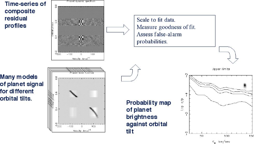
Figure 20: Schematic illustration of the main steps in the matched-filter analysis.

To detect the planet we must co-align and add its signal from profiles at many different orbit phases. Given an assumed orbital inclination, we can compute the sinusoidal path that the planet should follow through velocity space, together with the attendant changes in signal strength. To search for a pattern of faint features displaying the expected behaviour, we construct a set of matched filters that can be scaled to fit the data for each member of a set of appropriate orbital inclinations, as shown schematically in Fig. 20.

We model the velocity profile of the reflected-light signal as a sequence of gaussians with appropriate velocities and relative amplitudes:

$$G(v,\phi|K_{p}) = \frac{W_{\star}}{\Delta v_{p}\sqrt{2\pi}}g(\phi,i)\times$$ (26)

$$\exp\left[-\frac{1}{2}\left(\frac{v-K_{p}\sin\phi}{\Delta v_{p}}\right)^{2}\right].$$

The amplitude $K_{p}$ of the sinusoidal velocity variation is determined by the system inclination and stellar mass according to

$$K_{p}\simeq 139\left(\frac{M_{\star}}{1.3M_{\odot}}\right)^{1/3}\sin{i}{\rm km~{}s}^{-1}.$$ (27)

The phase angle $\alpha$ can be determined at any orbital phase from

$$\cos\alpha=-\sin i.\cos 2\pi\phi.$$ (28)

$W_{\star}$ is the integrated area of the deconvolved stellar line profile, and $\Delta v_{p}$ is the characteristic width of the planet’s reflected-light profile. The width $\Delta v_{p}=9.1$ km s^-1 of the gaussian representing the planetary profile was determined from a fit to the deconvolved profile of $\upsilon$ And.

D.1 Phase function

For the phase function there are two natural choices. First, the phase function of a Lambert sphere is

$$g(\alpha)=(\sin\alpha+(\pi-\alpha)\cos\alpha)/\pi.$$ (29)

This assumes that the planetary atmosphere scatters isotropically into $2\pi$ steradians.

Second, it may be more realistic to adopt a phase function that resembles those for the cloud-covered surfaces of planets in our own solar system. Jupiter and Venus appear to have phase functions that are more strongly back-scattering than a Lambert sphere. Photometric studies of Jupiter at large phase angles from the Pioneer and subsequent missions have shown (?) that the phase function for Jupiter is very similar to that of Venus. As a plausible alternative to the Lambert-sphere formulation, we use a polynomial approximation to the empirically determined phase function for Venus (?). The phase-dependent correction to the planet’s visual magnitude is approximated by:

$$\Delta m(\alpha)=0.09(\alpha/100^{\circ})+2.39(\alpha/100^{\circ})^{2}-0.65(\alpha/100^{\circ})^{3}.$$ (30)

so that

$$g(\alpha)=10^{-0.4\Delta m(\alpha)}.$$ (31)

D.2 Attenuation during starlight subtraction

The template spectrum that is subtracted in turn from each spectrum contains a blurred planet signal, as described in Appendix A. Our matched filter must therefore mimic accurately the effects of subtracting a template constructed from the spectra themselves, so we subtract the inverse variance-weighted average of the travelling gaussian. If $\sigma^{2}_{ij}$ is the variance of the $i$th velocity bin in the $j$th deconvolved profile, then the attenuated basis function becomes:

$$h_{ij}(K_{p})=G(v_{i},\phi_{j}|K_{p})-\frac{\sum_{j}G(v_{i},\phi_{j}|K_{p})/\sigma^{2}_{ij}}{\sum_{j}1/\sigma^{2}_{ij}}.$$ (32)

To allow for any systematic errors in the continuum level following template subtraction and deconvolution, we subtract the inverse variance-weighted mean value of each of the deconvolved profiles at each orbital phase. If $d_{ij}$ is the original data value at velocity $i$ and phase $j$, then

$$D_{ij}=d_{ij}-\frac{\sum_{i}d_{ij}/\sigma^{2}_{ij}}{1/\sigma^{2}_{ij}}$$ (33)

gives the resulting orthogonalised data pixel value. The matched filter is orthogonalised in the same way:

$$H_{ij}=h_{ij}-\frac{\sum_{i}h_{ij}/\sigma^{2}_{ij}}{1/\sigma^{2}_{ij}}.$$ (34)

D.3 Scaling the matched filter

The attenuated basis function $H(v,\phi,K_{p})$ is normalised such that when it is scaled to give an optimal fit to the entire time-series of $D_{ij}$ values, the scaling factor is $\epsilon_{0}$, the planet/star flux ratio at $\alpha=0$ as defined in eq. 15.

The optimal scale factor $\epsilon_{0}$ and its formal error are determined from

$$\epsilon_{0}(K_{p})=\sum_{i,j}\frac{D_{ij}H_{ij}(K_{p})/\sigma^{2}_{ij}}{H_{ij}^{2}(v_{i},\phi_{j},K_{p})/\sigma^{2}_{ij}}$$ (35)

and

$$\mbox{Var}(\epsilon_{0})=\sum_{i,j}\frac{1}{H_{ij}^{2}(K_{p})/\sigma^{2}_{ij}}.$$ (36)

We exclude all pixels within 25 km s^-1 of the stellar line core from the summations, to eliminate spurious effects arising from the ripple pattern in the core of the residual deconvolved stellar profile.

D.4 Calibrating non-grey albedo models.

The meaning of $\epsilon_{0}$ in the expressions above is obvious if the albedo spectrum is grey, i.e. if $\epsilon_{0}$ is independent of wavelength. Problems arise, however, when we wish to test how well a given non-grey albedo spectrum fits the data. In this case, the weighting factors $w_{i}$ used for the lines in the deconvolution mask mask are multiplied by the albedo as described in Appendix C above, and $\epsilon_{0}$ follows the wavelength dependence of the geometric albedo.

We circumvented this difficulty by replacing $\epsilon_{0}$ with $(R_{p}/a)^{2}$ as the scaling factor in eq. 35.

The basis function $G$ is rescaled to become $G^{\prime}=\left<p\right>G$, where $\left<p\right>$ is an appropriately weighted wavelength-averaged geometric albedo, then attenuated as before using eq. 32. For each candidate albedo spectrum we determine the appropriate value of $\left<p\right>$ empirically. We inject an artificial planet signal with the required albedo spectrum and known $K_{p}$ and $R_{p}/a$ into the data, and deconvolve the synthetic data with the albedo-weighted line list. We subtract the profiles of the observed spectra, following deconvolution with the same line list, to isolate the deconvolved planet signal from the noise. We then back-project the isolated planet signal, and measure the value of $\left<p\right>$ that recovers the correct value of $R_{p}/a$ at the appropriate $K_{p}$.

Appendix E False-alarm probabilities for candidate signals

Candidate reflected-light signals are characterised by positive values of $(R_{p}/a)^{2}$ and an improvement in $\chi^{2}$ relative to the fit obtained when $(R_{p}/a)^{2}=0$. We determine the frequency with which $(R_{p}/a)^{2}$ exceeds a given value due to noise in the absence of a planet signal, using a bootstrap procedure.

In each of 3000 trials, we randomize the order in which the three nights of observations were secured, then we randomise the order in which the observations were secured within each night. The re-ordered observations are then associated with the original sequence of dates and times. This ensures that any contiguous blocks of spectra containing similar systematic errors remain together, but appear at a new phase. Any genuine planet signal present in the data is, however, completely scrambled in phase. The re-ordered data are therefore as capable as the original data of producing spurious detections through chance alignments of blocks of systematic errors along a single sinusoidal path through the data. We record the least-squares estimates of $(R_{p}/a)^{2}$ and the associated values of $\chi^{2}$ as functions of $K_{p}$ in each trial. The 3000 trials implicitly define empirical probability distributions of $(R_{p}/a)^{2}$ and $\chi^{2}$ that include both the photon statistics and the effects of correlated systematic errors at each trial value of $K_{p}$.

The percentile points of the distribution of $(R_{p}/a)^{2}$ values at each $K_{p}$ are used to define the 1$\sigma$, 2$\sigma$, 3$\sigma$ and 4$\sigma$ upper-limit contours shown in Figs. 10, 11, 10, 14 and 17.

To assess the false-alarm probability for a candidate detection, however, we need to examine the likelihood of the fit to the data. In each bootstrap trial, the most likely candidate is the one among those with $(R_{p}/a)^{2}>0$ that yields the greatest improvement $\Delta\chi^{2}$ relative to the no-planet hypothesis. Such a peak can occur at any value of $K_{p}$. We use the distribution of the peak $\Delta\chi^{2}$ value in each trial to determine how often we would expect the $\Delta\chi^{2}$ of the strongest spurious noise feature giving $(R_{p}/a)^{2}>0$ to exceed the actual $\Delta\chi^{2}$ of a candidate detection in the observed data. We define this probability – summed over all possible values of $K_{p}$ with some weighting according to prior probability estimates – to be the “false-alarm probability” for a candidate signal.

The unweighted false-alarm probabilities are based on the likelihood of obtaining the data ${D}$ at a given $K_{p}$ after optimizing $(R_{p}/a)^{2}$, and take no account of whether or not that value of $K_{p}$ is plausible. This conditional likelihood is measured relative to the likelihood of getting the same data if no planet signal is present:

$$\frac{P(\mbox{\boldmath${D}$}|K_{p})}{P(\mbox{\boldmath${D}$}|\mbox{No planet})}=e^{-(\chi^{2}(K_{p})-\chi^{2}(\mbox{No planet}))/2},$$ (37)

where we have implicitly optimised the value of $(R_{p}/a)^{2}$ using the matched-filter fit at each $K_{p}$.

We take our prior knowledge of $K_{p}$ into account by modifying the likelihood to give the joint probability

$$P(\mbox{\boldmath${D}$},K_{p})=P(\mbox{\boldmath${D}$}|K_{p})P(K_{p}).$$ (38)

We use the prior probability distribution for $K_{p}$ as shown projected on to the $K_{p}$ axis in Fig.2.

We compute $P(\mbox{\boldmath${D}$},K_{p})$ for each of the 3000 bootstrap trials. To do this, we pick out the greatest value in each trial of the quantity

$$\ln P(\mbox{\boldmath${D}$},K_{p})=\ln P(K_{p})+\frac{\Delta\chi^{2}}{2}$$ (39)

where $P(K_{p})$ is derived from the simulations described in Section 2. The cumulative distribution of maximal $\log P(\mbox{\boldmath${D}$},K_{p})$ values derived from the bootstrap trials gives the probability that the observed peak value of $\ln P(\mbox{\boldmath${D}$},K_{p})$ could be spurious.

References

- Baliunas et al. 1997 Baliunas S. L., Henry G. W., Donahue R. A., Fekel F. C., Soon W. H., 1997, ApJ, 474, L119
- Brown et al. 2001 Brown T. M., Charbonneau D., Gilliland R. L., Noyes R. W., Burrows A., 2001, ApJ, 552, 699
- Burrows et al. 1997 Burrows A. et al., 1997, ApJ, 491, 856, Provided by the NASA Astrophysics Data System
- Burrows et al. 2000 Burrows A., Guillot T., Hubbard W. B., Marley M. S., Saumon D., Lunine J. I., Sudarsky D., 2000, ApJ, 534, L97
- Butler et al. 1999 Butler R. P., Marcy G. W., Fischer D. A., Brown T. M., Contos A. R., Korzennik S. G., Nisenson P., Noyes R. W., 1999, ApJ, 526, 916
- Charbonneau et al. 1999 Charbonneau D., Noyes R. W., Korzennik S., Nisenson P., Jha S., Vogt S. S., Kibrick R. I., 1999, ApJ, 522, L145
- Charbonneau et al. 2000 Charbonneau D., Brown T. M., Latham D. W., Mayor M., 2000, ApJ, 529, L45
- Collier Cameron et al. 1999 Collier Cameron A., Horne K. D., Penny A. J., James D. J., 1999, Nat, 402, 751
- Collier Cameron et al. 2001 Collier Cameron A., Horne K., James D. J., Penny A. J., Semel M., 2001, in Penny A., Artymowicz P., Lagrange A.-M., Russell S., eds, IAU Symp. 202: Planetary systems in the Universe. ASP Conference Series, San Francisco, In press: astro-ph0012186
- Donati et al. 1997 Donati J.-F., Semel M., Carter B., Rees D. E., Collier Cameron A., 1997, MNRAS, 291, 658
- Ford, Rasio & Sills 1999 Ford E. B., Rasio F. A., Sills A., 1999, ApJ, 514, 411
- Fuhrmann, Pfeiffer & Bernkopf 1998 Fuhrmann K., Pfeiffer M. J., Bernkopf J., 1998, A&A, 336, 942
- Gonzalez 1997 Gonzalez G., 1997, MNRAS, 285, 403
- Gonzalez 1998 Gonzalez G., 1998, A&A, 334, 221
- Guillot et al. 1996 Guillot T., Burrows A., Hubbard W. B., Lunine J. I., Saumon D., 1996, ApJ, 459, L35
- Guillot et al. 1997 Guillot T., Saumon D., Burrows A., Hubbard W. B., Lunine J. I., Marley M. S., Freedman R. S., 1997, in Cosmovici C. V., Bowyer S., Wertheimer D., eds, IAU Colloquium 161: Astronomical and biochemical origins and the search for life in the Universe. Editrice Compositori, Bologna, p. 343
- Henry et al. 2000 Henry G. W., Baliunas S. L., Donahue R. A., Fekel F. C., Soon W., 2000, ApJ, 531, 415
- Hilton 1992 Hilton J. L., 1992, in Seidelmann P. K., ed, Explanatory supplement to the Astronomical Almanac. University Science Books, Mill Valley, CA, p. 383
- Horne 1986 Horne K. D., 1986, PASP, 98, 609
- Hovenier & Hage 1989 Hovenier J. W., Hage J. I., 1989, A&A, 214, 391
- Kupka et al. 1999 Kupka F., Piskunov N., Ryabchikova T. A., Stempels H. C., Weiss W. W., 1999, A&AS, 138, 119
- Marcy & Butler 1998 Marcy G. W., Butler R. P., 1998, ARA&A, 36, 57
- Marley et al. 1999 Marley M. S., Gelino C., Stephens D., Lunine J. I., Freedman R., Sharp C., 1999, ApJ, 513, 879
- Marsh 1989 Marsh T. R., 1989, PASP, 101, 1032
- Mayor & Queloz 1995 Mayor M., Queloz D., 1995, Nat, 378, 355
- Noyes et al. 1984 Noyes R. W., Hartmann L., Baliunas S. L., Duncan D. K., Vaughan A. H., 1984, ApJ, 279, 763
- Perryman et al. 1997 Perryman M. A. C. et al., 1997, A&A, 323, L49
- Press et al. 1992 Press W. H., Flannery B. P., Teukolsky S. A., Vetterling W. T., 1992, Numerical Recipes: The Art of Scientific Computing (2nd edition). Cambridge University Press, Cambridge
- Saumon et al. 1996 Saumon D., Hubbard W. B., Burrows A., Guillot T., Lunine J. I., Chabrier G., 1996, ApJ, 460, 993
- Seager & Sasselov 1998 Seager S., Sasselov D. D., 1998, ApJ, 502, L157
- Sudarsky, Burrows & Pinto 1999 Sudarsky D., Burrows A., Pinto P., 1999, ApJ, 538, 885