X-Ray Spectral and Timing Observations of Cygnus X-2
Abstract
We report on a joint BeppoSAX/RossiXTE observation of the Z-type low mass X-ray binary Cyg X–2. The source was in the so-called high overall intensity state and in less than 24 hours went through all three branches of the Z–track. The continuum x-ray spectrum could be described by the absorbed sum of a soft thermal component, modeled as either a blackbody or a multicolor disk blackbody, and a Comptonized component. The timing power spectrum showed several components including quasiperiodic oscillations in the range 28–50 Hz while the source was on the horizontal branch (horizontal branch oscillation; HBO). We found that the HBO frequency was well correlated with the parameters of the soft thermal component in the x-ray spectrum. We discuss implications of this correlation for models of the HBO.
1 Introduction
Cygnus X–2 is a bright persistent Low–Mass X–ray Binary (LMXB). It consists of a neutron star, having the highest optically measured mass reported to date ( , Casares, Charles & Kuulkers 1998), orbiting the evolved, late–type companion V1341 Cyg, with a period of days (Cowley, Crampton & Hutchings 1979; Casares, Charles & Kuulkers 1998). Although Cyg X–2 is one of longest know and best studied LMXBs, a clear understanding of its behavior has not yet been obtained.
Cyg X–2 is classified as a Z-source due to its behavior when studied on an x-ray color-color diagram (CCD). Z-sources follow a one-dimensional trajectory in the two-dimensional CCD, tracing out a Z shape as the source evolves between different spectral states. The parts of the Z are referred to as the horizontal branch (HB) at the top of the Z, the normal branch (NB) along the diagonal of the Z, and the flaring branch (FB) at the base of the Z. Z-sources move continuously along the Z-diagram and the position of the source within the Z is believed, from simultaneous multi-band (radio, UV, optical and X–ray) observations (Hasinger et al. 1990), to be related to the mass accretion rate with accretion at a minimum at the left end of the HB and at a maximum at the right end of the FB. However, the behavior of Z-sources is not described by a single parameter because, on time scale of weeks to months, the morphology and position of the Z-track in the CCD vary. Kuulkers et al. (1996) described the phenomenology for Cyg X–2 in terms of three overall intensity levels (high, medium, and low), with different morphology for the Z track in the different intensity levels.
Z-sources, including Cyg X–2, show complex X-ray spectrum, requiring a superposition of several spectral components. Different composite models, including thermal bremsstrahlung together with blackbody radiation, two blackbodies, a power law plus thermal bremsstrahlung, a multi–temperature blackbody disk plus boundary layer blackbody, or a Comptonized spectrum, have all been found to describe adequately the data. Unfortunately, spectral modeling alone has not led to unique identification of the physical origin of the various spectral components. Further observations relating the x-ray spectra to other other source parameters are required.
Z-sources also show rich X-ray timing power spectra including several components and varying with position in the CCD. Cyg X–2 shows quasiperiodic oscillations (QPOs) with frequency varying between Hz and Hz, present on the horizontal branch and on the upper part of the normal branch (HBOs), and high frequency QPOs (kHz QPOs), ranging between 300 Hz and 900 Hz have been detected on the HB (Wijnands et al. 1998). Slower QPOs with frequencies of 5–7 Hz are observed on the lower part of the normal branch (called NBOs). Sometime HBOs are observed simultaneously with the NBOs, indicating these QPOs should be produced by different mechanisms. Agreement is lacking on a unique model to explain the HBOs, the NBOs, or the kHz QPOs. Correlations between the timing parameters and other source parameters may help limit the number of viable models for the QPOs.
In this paper, we present joint timing and spectral observations of Cygnus X–1 obtained with RossiXTE and BeppoSAX. The goal of our observations was to obtain simultaneous x-ray spectral and timing data for Cyg X-2 in order to study correlations between the spectral and timing parameters. The observations and analysis are described in §2. Results on the color and intensity evolution are presented in §3, on timing power spectra in §4, and on energy spectra in §5. The correlations between spectral and timing properties is described in §6. We discuss the implications of our results in §7.
2 Observations and Analysis
On 2000 June 2–3, we performed a joint observation of Cyg X–2 with the RossiXTE and BeppoSAX satellites. The pointing was carried out between 2000 June 2 13:11 UT and June 3 17:23 UT, with RossiXTE (Bradt et al. 1993) and between 2000 June 2 18:56 UT and June 3 14:25 UT with the BeppoSAX Narrow Field Instruments, NFIs (Boella et al. 1997).
Spectral data obtained from the RXTE Proportional Counter Array (PCA) in 129 photon energy channels with a time resolution of 16 s (standard 2) were used to extract a color-color diagram (CCD) and a hardness-intensity diagram (HID). The soft and hard colors were defined as counts rate ratios between 4.0–6.4 keV and 2.6–4.0 keV and between 9.7–16 keV and 6.4–9.7 keV. The intensity was defined as the PCU2 count rates in the energy band 2.6–16 keV. All count rates were background subtracted. We used only PCU2 for the intensity and color analysis as only it and PCU0 were on during all observations and PCU0 suffered from a propane layer leak which made the energy calibration very uncertain.
Timing data obtained from the PCA with a time resolution of 125 in Single Bit (one energy channel) modes for the energy bands 2.0–5.8 keV, 5.8–10.1 keV, 10.1–21.4 keV, and 21.4–120 keV were used to obtain power spectra. We note that the data mode used does not allow us to remove events from PCU0. Thus, due to the propane layer leak, the true energy bands for PCU0 likely differ from these nominal ranges. However, our basic result on the energy dependent of the timing noise (that the noise features are stronger at higher energies) is not sensitive to the details of the energy band boundaries.
To search for fast kHz QPOs, we performed Fast Fourier transforms on 2 s segments, added all power spectra obtained within each selected observation interval, and then searched for excess power in the 200–2048 Hz range. No kHz QPOs with a chance probability of occurrence of less than were found either in the full band data or in the data above 5.8 keV. The kHz QPO previously found from Cyg X–2 occurred in the medium overall intensity state (Wijnands et al. 1998). No kHz QPOs have been observed during the high intensity state.
To study the low frequency behavior, we performed Fast Fourier transforms on 64 s segments and we added the 64 s power spectra obtained for all or the three highest energy bands within each continuous observation interval. The expected Poisson noise level, due to counting statistics, was estimated taking into account the effects of the deadtime and subtracted from each power spectrum, and the power spectra were normalized to fractional rms. Each 0.1–100 Hz total power spectrum was fitted as described below.
Data from the BeppoSAX NFIs were used to extract broad band energy spectra. The NFIs are four coaligned instruments covering the 0.1–200 keV energy range: LECS (0.1–10 keV), MECS (1.3–10 keV), HPGSPC (7–60 keV), and PDS (13–200 keV). The net on–source exposure times were 11 ks, 27 ks, 35 ks and 20 ks for LECS, MECS, HPGSPC, and PDS respectively. LECS and MECS data were extracted in circular regions centered on Cyg X–2’s position having radii of and respectively. The same circular regions in blank field data were used for the background subtraction. Cyg X–2 is sufficiently bright during this observation that the background subtraction does not affect the fits results. Spectra accumulated from Dark Earth data and during off–source intervals were used for the background subtraction in the HPGSPC and in the PDS respectively. The LECS and MECS spectra have been rebinned to sample the instrument resolution with the same number of channels at all energies. Logarithmic rebinning was used for the HPGSPC and PDS spectra.
We investigated the source power and energy spectrum in different regions of the HID. Energy spectra of each NFI were create over five different HID intervals where BeppoSAX data were present. These spectra are indicated with E, F, C, B, A and reported in order of position along the Z track in Tables 3 and 4. The alphabetical order indicates the sequence in time (see MECS light curve in Figure 2).
3 Color and Intensity Evolution
Figure 1 shows the RXTE ASM light curve of Cygnus X–2 where the long–term X-ray variation is clearly visible. The time of the RXTE/BeppoSAX observation is indicated with an arrow on the right. The light curve around the observation (see the inset in Figure 1) shows complex time variability. The source was in the high overall intensity state (Kuulkers, van der Klis & Vaughan 1996) and during the observation moved along the three branches of the Z pattern (this is more evident in the HID than in the CCD). No x-ray bursts occurred during the observation.
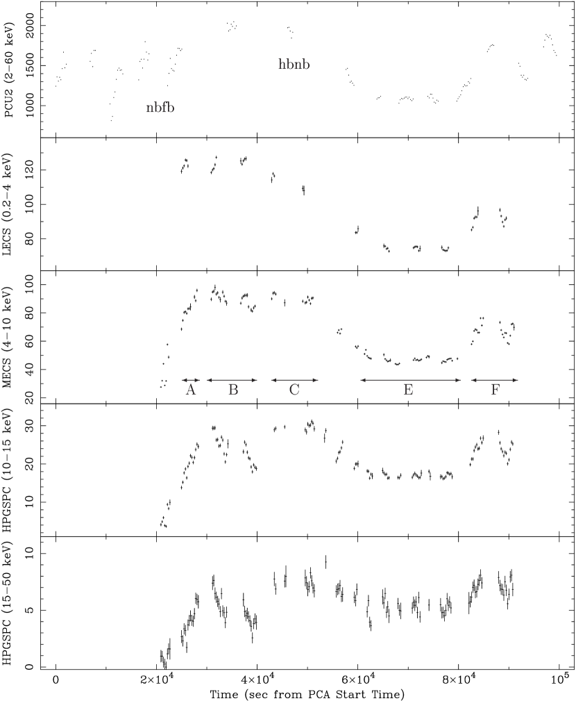
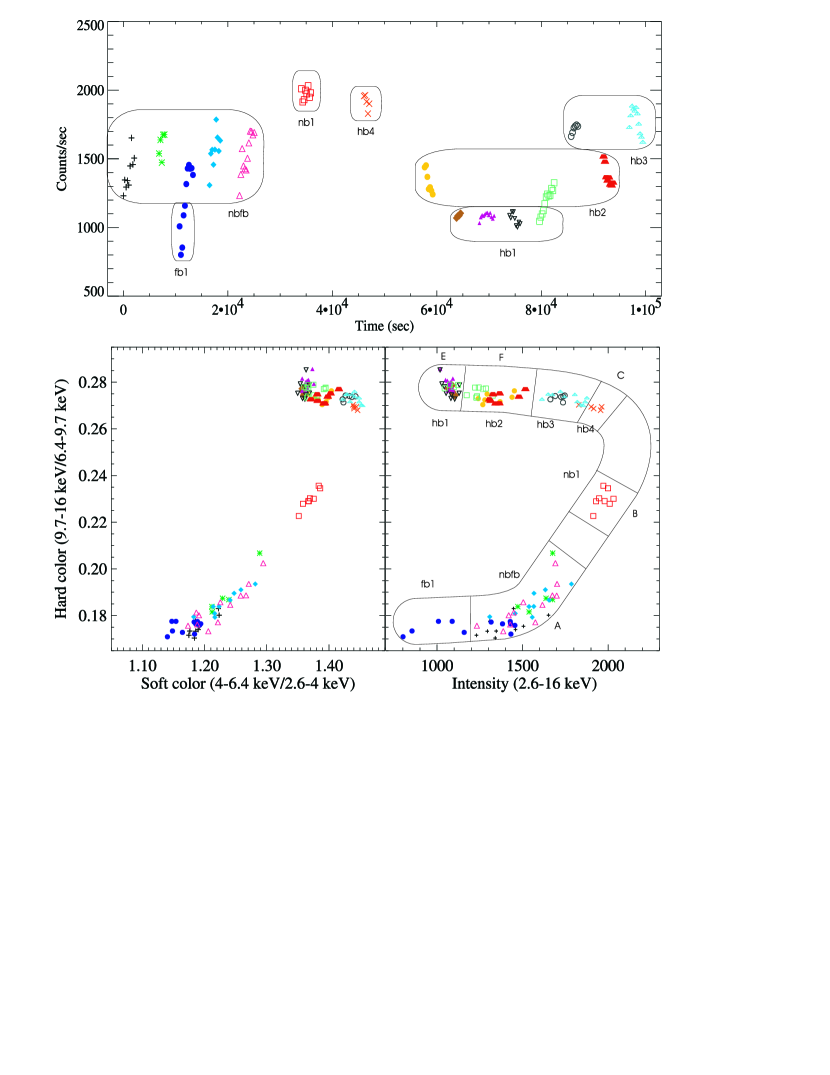
The RXTE/BeppoSAX light curves obtained in the entire energy range of the PCU2 and the various energy ranges of the NFIs are shown in Figure 2, and Figure 3 shows the color-color (CCD) and hardness-intensity (HID) diagrams. The bin size is 256 s. In Figure 3, each symbol indicates a different continuous segment in the light curve (see upper panel).
The states of Z sources are typically described in terms of a horizontal branch (HB), a normal branch (NB), and a flaring branch (FB), as described above. The HB consists of the points with high hardness and varying intensity in the HID, the NB has high intensity and varying hardness, and the FB has low hardness and varying intensity. As observed during other high intensity levels (Wijnands et al. 97, Wijnands & van der Klis 2001) the FB in HID is almost horizontal and the correlation of intensity with position along the Z track reverses in the FB relative to the HB. We divided the data into seven states for use in the analysis below. Four regions are in the HB (marked as hb1, hb2, hb3, hb4 on the HID) one is in the NB (nb1), one region is at the NB/FB corner (nbfb), and finally one is in the FB (fb1).
The overall intensity of the source changes by more than a factor of 2 during the entire observation (see the PCU2 light curve). The character of the intensity variations changes with energy. Just after the beginning of the BeppoSAX observation, near a time of and marked as nbfb in Figure 2, the source moved from the flaring branch (FB) to the normal branch (NB) and the counts rates increased by more than a factors of 5 in the 4–10 keV, 10–15 keV, 15–50 keV energy ranges but remained roughly constant in the 0.2–4 keV band. Conversely, near a time of , and marked as hbnb in Figure 2, the source crossed the NB/HB corner and the count rates in the bands below 10 keV suffer large decreases, while the rate in the 15–50 keV band remains decreases only slightly.
4 Fast Timing
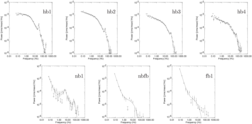
To investigate the evolution of fast timing behavior with position in the HID, we created power spectra in 7 regions of the HID described above and shown in Figure 3. The resulting power spectra obtained from the full PCA band are shown in Figure 4 and power spectra obtained using events from the three higher energy single-bit channels, i.e. photons with energies above 5.8 keV, in Figure 5.
At least five different power spectral components have been distinguished in the power spectra of Cygnus X–2 and other Z sources (Hasinger and van der Klis 1989): 1) a power law which is referred to as Very Low Frequency Noise (VLFN) because it dominates below 0.1 Hz; 2) a broad noise component, referred as Low Frequency Noise (LFN), represented by a flat power law with a high frequency cutoff, which characterizes the HB power spectra up to around 10 Hz; 3) a broad noise component having a similar shape as LFN, but extending to 100 Hz or above, known as High Frequency Noise (HFN), present in all spectral states; 4) a narrow excess with centroid frequency in the 15–60 Hz range, present in the HB, called the horizontal branch oscillation (HBO), and modeled with a Lorentzian; 5) another broad peak present in the NB, similar in shape to HBO, but with a characteristic frequency of around 6 Hz, called the normal branch oscillation (NBO). The solid curves in Figures 5 and 6 represent analytic fits consisting of these components. The components used for each power spectrum and the fit parameters obtained are presented in Tables 1 and 2. The fractional rms amplitude for the VLFN component was found by integrating over the frequency range 0.001–1 Hz. A range of 0.01–100 Hz was used for both LFN and HFN components. Because the HFN powerlaw index been found to be consistent with zero in Z sources (Hasinger & van der Klis 1989), we fixed it to zero.
A strong narrow HBO is present at the left end of the HB (hb1). A faint and narrow feature was visible in the first three HB power spectra near the position of the second harmonic, and there is also a possible third harmonic in the hb1 power spectrum. Moving along the HB towards the NB, the frequency increased from 28 Hz to 50 Hz, while its rms amplitude decreased from 2.8 to 1.7 (for keV, the rms decreased from 4.3 to 2.4 ), and its width increased from 6.7 Hz to 16.5 Hz. This behavior is consistent with that observed in the Ginga data by Wijnands et al. (1997).
LFN and HFN can be identified in all 4 HB power spectra. The VLFN was not fitted separately from LFN because its power in the 0.1–100 Hz range was much smaller than that of LFN. The rms of the LFN was 4–5% (6–7% for keV) and changed little along the HB. The powerlaw index and the cut–off frequency showed a positive correlation with the HBO frequency. The HFN component showed a cutoff frequency which is consistent with constant within the (sometimes large) errors, and a clear inverse correlation between its strength and the HBO frequency.
On the upper part of the NB (nb1), the HBO is still visible at 54 Hz with an rms level of 1.8% (3.1% for kev). In addition, a broad NBO is present at 5 Hz. The NBO feature is lost in the continuum as the source moved towards the FB. A very strong VLFN component (rms up to ) replaced the LFN in the continuum of the NB and FB power spectra. The VLFN became stronger moving from the NB to the FB, and the HFN showed the opposite trend.
5 Spectral Results
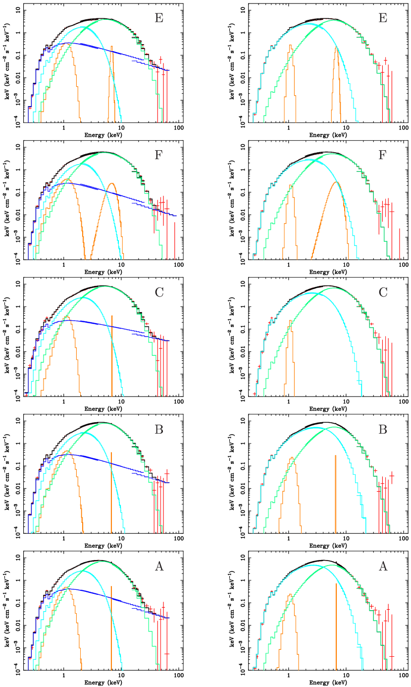
To investigate the spectral behavior versus the position on the Z track, we created energy spectra in 5 regions of the HID described above. We fitted the X-ray continuum of Cyg X–2 with several two–component models. A blackbody or disk multicolor blackbody (diskbb, Mitsuda et al. 1984) was used to model the soft component, and one of three thermal Comptonization models, a power law with cutoff, or the solution of the Kompaneets equation given by Sunyaev & Titarchuk 1980 compst or its improved version comptt (in which relativistic effects are included, Titarchuk 1994), was used for the harder component. The addition of a gaussian around 1 keV was required in all intervals. Lines near 1 keV have been observed previously from Cyg X-2 with instruments with higher resolution (Vrtilek et al. 1988). We also included a gaussian near 6.7 keV to model possible Fe emission lines. The best fit to the continuum of Cyg X–2 was obtained using a blackbody or a diskbb plus the comptt Comptonization model (thereafter we call bb+comptt and diskbb+comptt).
Using the diskbb+comptt model (Table 4, plots on the right in Figure 7) adequate fits were obtained. There is a slight, but not statistically significant excess of counts at high energy in the E and F spectra. The parameters of the diskbb component varied significantly with position along the Z track with the inner disk temperature, , changing from 0.79 keV to 1.07 keV, and the inner radius changing from 63 km to 47 km. Strong correlations of the parameters of the comptt component, other than its flux, with position along the Z track were not evident. The temperature and effective Wien radius of the seed photons for the Comptonized component were constant at keV and . The temperature of the Comptonizing region was also roughly constant at keV, while the optical depth varied in the range .
With the bb+comptt model, an excess of counts above keV was apparent in all five spectra. Because it is now known that a hard tail is sometimes present in the spectra of Z sources, we added a powerlaw component to fit the hard tail. Addition of the powerlaw is justified by the F-test statistic (the probability that the improvement in is due to chance is always less than ). This additional component was detected up to energies of keV, had a best fit photon index and contributed of the 0.1-100 keV source flux.
Hard tails have been reported in the spectra of Z sources, including for GX 5-1 using Ginga by (Asai et al. 1994), for Cyg X-2 using BeppoSAX (Frontera et al. 1998) , for Sco X-1 using CGRO/OSSE (Strickman & Barret 2000) and using RXTE/HEXTE (D’Amico et al. 2001a), and for GX 17+2 (Di Salvo et al. 2000), GX 349+2 (Di Salvo et al. 2001), and Cir X-1 (Iaria et al. 2001) using BeppoSax observations. The need for a hard powerlaw tail in the present data depend on the choice of the spectral model, and, thus, cannot be considered a detection of the hard powerlaw tail. D’Amico et al. (2001b), taking into account all the results on the detections of hard X-ray tails in Sco X-1 and GX 349+2, argue that the appearance of a such component is correlated with the brightness of the thermal component. Specifically, they propose that the production of a hard X-ray tail in a Z source is a process triggered when the thermal component is brighter than a level of 4 1036 ergs s-1 in the 20–50 keV energy range. In this energy range, the luminosity of Cyg X-2, in the observation discussed here, was 4.5 1036 ergs s-1, i.e. very close to the trigger value. Hence, our results appear consistent with previous observations. However, the fact that the hard powerlaw component is not required in the diskbb+comptt model underscores the importance of understanding the low energy emission in modeling the hard x-ray emission from x-ray binaries.
Results from these three-component fits to the BeppoSAX spectra of Cyg X–2 are given in Table 3 and in the plots on the left in Figure 7. Because the powerlaw normalization, absorption column , and Luminosity, obtained by fitting the E segment energy spectrum, were surprisingly higher than in other segments, we also report the fit parameters obtained by fixing the value to 2 cm-2, close to the average value from the other observations. The blackbody flux is well correlated with position along the Z track. The blackbody temperature and equivalent radius were approximately constant at keV and km (using a distance of 11.6 kpc, Casares et al. 1999), respectively. The temperature of the seed photons for the Comptonized component was roughly constant at keV. Following In ’t Zand et al. (1999), we derived an effective Wien radius of the seed photons; this was roughly constant at km. The temperature and optical depth of the (spherical) Comptonizing region were keV and , respectively.
The addition of an Fe Kα line at keV proved necessary, especially when the source was in the HB (spectra E and F). Similar parameters for the line where found using both the bb+comptt and diskbb+compTT models. BeppoSAX does not have adequate spectral resolution to draw detailed conclusions about the origin of this line (Piraino, Santagelo, & Kaaret 2000), but the presence of the line is motivation for high resolution spectral studies of Cyg X-2 while in the HB.
6 Correlation of Spectral and Timing Parameters
To directly compare the spectral and timing properties of Cyg X-2, we performed a second timing analysis of the RXTE data using regions of the Z-diagram matching the regions selected for spectral analysis. The analysis was performed as described above. In Figure 8, we plot the spectral parameters obtained for the Comptonization and thermal components of the E, F, C, and B spectra for the two models discussed above versus the HBO frequency. The flux from the Compton component appears correlated with HBO frequency for the bb+compTT model, but may not be for the diskbb+compTT model. The other Comptonization parameters do not appear correlated with HBO frequency in either model. The total flux is clearly correlated with HBO frequency in both models. However, we note that these observations sample only a short time span and correlations between timing parameters and total flux are generally not robust over long intervals (Ford et al. 1997). Interestingly, a strong correlation exists between the parameters of the soft spectral component, either the blackbody flux for the bb+compTT model or the disk inner radius for the diskbb+compTT model, and the HBO frequency.
7 Discussion
We discovered a correlation between the HBO frequency and the parameters of the soft thermal spectral component – the blackbody flux for the blackbody model and the disk inner radius for the multicolor disk blackbody model. This likely implies a physical relation between the source of the soft thermal emission and the timing frequencies.
RXTE and BeppoSAX data from the atoll source 4U 0614+091, covering a span of more than one year, showed a robust correlation between the kHz QPO frequency and the flux of the blackbody component in data spanning several years (Ford et al. 1997; Piraino et al. 1999). Because the frequencies of the various timing signals from x-ray binaries appear to be highly correlated (Psaltis et al. 1999), the physical implications of the spectral-HBO correlation are likely to be similar to those of the spectral-kHz QPO correlation.
A correlation would occur naturally in models where the oscillation frequencies are related to the Keplerian orbital frequency, , at inner edge of the accretion disk, , (e.g. Alpar & Shaham 1985, Miller, Lamb & Psaltis 1998; Stella & Vietri 1998) and the flux from the soft thermal component arises from an accretion disk (the usual interpretation of the diskbb model). The Keplerian relation, , would be expected if the oscillation frequency, , is linearly related to the Keplerian orbital frequency, . We fitted a function of the form to the data with taken as the disk radius from the diskbb spectral component. The best fit exponent is which is consistent with the Keplerian value . With fixed to the Keplerian value, the coefficient . This is consistent with a neutron star if .
In the ‘magnetospheric beat–frequency model’ (e.g. Alpar & Shaham 1985; Psaltis et al. 1999) the centroid frequency of the QPO is identified with the difference between the Keplerian frequency at magnetospheric radius and the spin frequency, of the neutron star. If the inner disk radius is equal to the magnetospheric radius, then . Fitting this form to the data, we find and . These values are inconsistent with a neutron star mass above . However, we note that may not reflect the true magnetospheric radius.
The current data consist of only a few points, with significant errors on the derived spectral parameters for some of the points. Hence, the data are not sufficient to adequately constrain the relation between the oscillation frequency and the spectral parameters so that strong conclusions about the viability of particular models can be drawn. Additional observations with higher spectral resolution and better low energy response, made simultaneously with timing observations would be of great interest and might provide a means to discriminate between various models of the HBO.
References
- Alpar & Shaham (1985) Alpar, M. A. & Shaham, J. 1985, Nature, 316, 239
- Asai et al. (1994) Asai, K., Dotani, T., Mitsuda, K. et al. 1994, PASJ, 46, 479
- Boella et al. (1997) Boella, G., et al. 1997, A&A, 122, 299
- Bradt, Rothschild, & Swank (1993) Bradt, H. V., Rothschild, R. E., Swank, J. H., 1993, A&A, 97, 355
- Casares, Charles & Kuulkers (1998) Casares, J., Charles, P. & Kuulkers, E. 1998, ApJ, 493, L39
- Cowley, Crampton & Hutchings (1979) Cowley, A. P., Crampton, D. & Hutchings, J.B. 1979, ApJ 231, 539
- (7) D’Amico, F., Heindl, W. A, Rothschild, R. E., Gruber, D. E. 2001, ApJ, 547, L147
- (8) D’Amico, F., Heindl, W. A, Rothschild, R. E., Gruber, D. E. 2001, to appear in AIP Conf. Proc. of Gamma 2001 Symposium , astro-ph/0105201.
- Di Salvo et al. (2000) Di Salvo, T., Stella, L., Robba, N. R. et al. 2000, ApJ, 544, L119
- Di Salvo et al. (2001) Di Salvo, T., Robba, N. R., Iaria, R. et al. 2001, ApJ, 554, 49
- Ford et al. (1997) Ford, E. C., Kaaret, P., Chen, K., et al. 1997, ApJ, 486, L47
- Frontera et al. (1998) Frontera, F., Dal Fiume, D., Malaguti, G. et al. 1998, Nucl. Physics B (Proc. Suppl), 69, 286
- Hasinger & van der Klis (1989) Hasinger, G. and van der Klis, M. 1989, A&A, 225, 79
- Hasinger et al. (1990) Hasinger, G., van der Klis, M., Ebisawa, K. et al. 1990, A&A, 235, 131
- Iaria et al. (2001) Iaria, R., Burderi, L., Di Salvo, T. et al. 2001, 547, 412
- In’t Zand et al. (1999) In’t Zand, J. J. M., Verbunt, F. Strohmayer, T. E. et al. 1999, A&A, 345, 100
- Kuulkers & van der Klis (1995) Kuulkers, E. & van der Klis, M. 1995, A&A, 303, 801
- Kuulkers, van der Klis & Vaughan (1996) Kuulkers, E., van der Klis, M. & Vaughan, B. A. 1996, A&A, 311, 197
- Matt, Fabian, & Ross (1996) Matt, G., Fabian, A. C., Ross, R. R., 1996, MNRAS, 278, 1111
- Miller, Lamb & Psaltis (1998) Miller, M. C., Lamb, F. K. & Psaltis, D. 1998, ApJ, 508, 791
- Mitsuda et al. (1984) Mitsuda, K., Inoue, H., Koyama, K. et al. 1984, PASJ, 36, 741
- Piraino et al. (1999) Piraino, S., Kaaret, P., Santangelo, A., Ford, E. C. 1999, AAS, HEAD meeting 31, 15
- Piraino et al. (2000) Piraino, S., Santangelo, A., & Kaaret, P. 2000, A&A, 360, L35
- Psaltis, Belloni & van der Klis (1999) Psaltis, D., Belloni, T. & van der Klis, M. 1999, ApJ, 520, 262
- Raymond (1993) Raymond, J.C. 1993, ApJ 412, 267
- Stella & Vietri (1998) Stella L. & Vietri M., 1998, ApJ, 492, L59
- Sunyaev & Titarchuk (1980) Sunyaev, R. A. and Titarchuk, L. G. 1980, A&A, 86, 121
- Strickman & Barret (2000) Strickman, M. & Barret, D. 2000, in Proc. of the Fifth Compton Symposium, AIP Conf. Proc. 510, 222
- Titarchuk (1994) Titarchuk, L. 1994, ApJ, 434, 570
- Vrtilek et al. (1988) Vrtilek, S.D, Swank, J.H, Kallman, T.R. 1988, ApJ, 326, 186
- Wijnands et al. (1997) Wijnands, R., van der Klis, M., Kuulkers, E. et al. 1997, A&A, 323, 399
- Wijnands et al. (1998) Wijnands, R., Homan, J., van der Klis, M. et al. 1998, ApJ, 493, L87
- Wijnands & van der Klis (2001) Wijnands, R. and van der Klis, M. 2001, MNRAS, 321, 537


| Z | LFN | HFN | HBO | DOF | ||||||
|---|---|---|---|---|---|---|---|---|---|---|
| rms | rms | rms | ||||||||
| Hz | Hz | Hz | Hz | |||||||
| hb1 | ||||||||||
| hb2 | ||||||||||
| hb3 | ||||||||||
| hb4 | ||||||||||
| hb1h | ||||||||||
| hb2h | ||||||||||
| hb3h | ||||||||||
| hb4h | ||||||||||
| Z | VLFN | HFN | HBO | NBO | ||||||||
|---|---|---|---|---|---|---|---|---|---|---|---|---|
| rms | rms | rms | rms | |||||||||
| Hz | Hz | Hz | Hz | Hz | ||||||||
| nb1 | ||||||||||||
| nbfb | ||||||||||||
| fb1 | ||||||||||||
| nb1h | ||||||||||||
| nbfbh | ||||||||||||
| fb1h | ||||||||||||
| Spectrum | E | E ( fixed) | F | C | B | A |
|---|---|---|---|---|---|---|
| Z region | hb1 | hb1 | hb2 | hb4 | nb1 | nbfb |
| (keV) | ||||||
| (km) | ||||||
| (keV) | ||||||
| (keV) | ||||||
| (km) (d=11.6 kpc) | ||||||
| Photon Index | ||||||
| Power-law | ||||||
| (keV) | ||||||
| (keV) | ||||||
| (ph cm-2 s-1) | ||||||
| line (eV) | 44 | 176 | 242 | 115 | 186 | 181 |
| (keV) | ||||||
| (keV) | ||||||
| (ph cm-2 s-1) | ||||||
| Fe (eV) | 44 | 44 | 115 | 10 | 8 | 13 |
| ( ergs cm-2 s-1) | ||||||
| (ergs cm-2 s-1) | ||||||
| (ergs cm-2 s-1) | ||||||
| ( d=11.6 kpc) | 2.37 | 1.28 | 1.58 | 1.90 | 2.02 | 1.87 |
| (d.o.f.) | 1.68 (113) | 1.80 (114) | 1.19 (119) | 1.18 (117) | 1.09 (116) | 1.00 (115) |
| -test 1 (fe) | ||||||
| -test 2 (po) |
| Spectrum | E | F | C | B | A |
|---|---|---|---|---|---|
| Z region | hb1 | hb2 | hb4 | nb1 | nbfb |
| (keV) | |||||
| (D=d/10 kpc) | |||||
| (km) (d=11.6 kpc, ) | |||||
| (keV) | |||||
| (keV) | |||||
| (km) d=11.6 kpc | |||||
| (keV) | |||||
| (keV) | |||||
| Iline (ph cm-2 s-1) | |||||
| line Eq. W. (eV) | 33 | 28 | 19 | 37 | 35 |
| (keV) | |||||
| (keV) | |||||
| (ph cm-2 s-1) | |||||
| Fe (eV) | 48 | 140 | 8 | 17 | |
| ( ergs cm-2 s-1) | |||||
| ( ergs cm-2 s-1) | |||||
| (d=11.6 kpc) | 1.19 | 1.52 | 1.97 | 1.97 | 1.77 |
| (d.o.f.) | 1.72 (112) | 1.16 (118) | 1.34 (116) | 1.19 (112) | 1.25 (114) |