Heating and Ionization of X-Winds

Abstract

In order to compare the x-wind with observations, one needs to be able to calculate its thermal and ionization properties. We formulate the physical basis for the streamline-by-streamline integration of the ionization and heat equations of the steady x-wind. In addition to the well-known processes associated with the interaction of stellar and accretion-funnel hot-spot radiation with the wind, we include X-ray heating and ionization, mechanical heating, and a revised calculation of ambipolar diffusion heating. The mechanical heating arises from fluctuations produced by star-disk interactions of the time dependent x-wind that are carried by the wind to large distances where they are dissipated in shocks, MHD waves, and turbulent cascades. We model the time-averaged heating by the scale-free volumetric heating rate, $\Gamma_{\rm mech}=\alpha\rho v^{3}s^{-1}$, where $\rho$ and $v$ are the local mass density and wind speed, respectively, $s$ is the distance from the origin, and $\alpha$ is a phenomenological constant. When we consider a partially-revealed but active young stellar object, we find that choosing $\alpha\sim 10^{-3}$ in our numerical calculations produces temperatures and electron fractions that are high enough for the x-wind jet to radiate in the optical forbidden lines at the level and on the spatial scales that are observed. We also discuss a variety of applications of our thermal-chemical calculations that can lead to further observational checks of x-wind theory.

1 Introduction

A refined and updated version of the disk-accretion paradigm for the formation of Sun-like stars has emerged in the last two decades through extensive observations and theoretical studies. In addition to the building up of the new star by accretion from a disk formed by the collapse of a rotating molecular cloud core, the formation of a low-mass star is accompanied by a remarkable bipolar outflow that can appear jet-like at optical and nearby wavelengths. Equally important is the crucial role of magnetic fields in retarding the initial collapse and in guiding both the accretion flow that feeds the star and the outflow that removes excess angular momentum. In addition to the strong evidence provided by the essentially universal detection of X-rays in low-mass young stellar objects (YSOs), magnetic fields have been measured directly with the Zeeman effect (e.g., Johns-Krull and Valenti, 2000). Although the general outline of a theory of low-mass star formation has emerged, the underlying mechanisms still need to be identified and understood, and strong efforts along these lines are in progress on a broad front, as can be seen in the reports at the recent conference Protostars and Planets IV (Mannings, Boss, and Russell 2000).

One of the main goals of the theory is to develop a rational description of the active flows close to the central engine, i.e., the accretion funnel and the wind. Although there is a consensus that these flows are MHD in character, considerable disagreement exists over the specifics, as witnessed by the reviews of magnetocentrifugal winds at Protostars and Planets IV by Königl and Pudritz (2000; disk winds) and by Shu, Najita, Shang, and Li (2000; x-wind), as well as the earlier review of wind theory by Pudritz and Ruden (1993). Of course the only way to decide between alternative theories or to validate any particular theory is to make detailed comparisons with observations. Thus, it is the objective of the present paper to develop the basis for making such comparisons for the case of the x-wind (Shu et al. 1994a; Shu et al. 1994b; Najita & Shu 994; Ostriker & Shu 1995; Shu et al. 1995; henceforth Papers I-V). The x-wind model has the potential for understanding many aspects of low-mass star formation because it provides well-defined dynamical solutions that can be used to make detailed correlations and predictions of observational data. It should be clear that, because x-wind theory focuses on the inner region (or “central engine”) of the star in formation of dimension 0.1 AU, observational tests require spectroscopy on the milli- arc-second spatial scale and better. Such observations are now becoming available with adaptive optics and interferometric techniques, as well as with the Hubble Space Telescope.

As discussed by Shu et al. (2000), several crucial assumptions and implications of the x-wind model are supported by observations: the existence of a finite inner radius for a rapidly rotating inner disk; strong magnetization of the central star; magnetically channeled accretion; and phase relations between stellar rotation and the accretion funnel and the outflow. The model can also account for the large-scale kinematic properties of bipolar molecular outflows (Shu et al. 1991, 2000), and it has the potential to explain the optical observations of jets from young stellar objects. The latter possibility is a consequence of the remarkable property of the x-wind, whose 180^∘ bipolar lobes self-collimate towards the outflow axis into approximately cylindrical jets (Paper V). On this basis, Shang, Shu, & Glassgold (1998, henceforth SSG) made synthetic images of optical jets that bear a striking resemblance to the observed ones (see, e.g., Eislöffel et al. 2000).

These conclusions have been made on the basis of the dynamical solution of the x-wind model which gives the density, velocity, and magnetic field configuration. The images obtained by SSG were obtained by using constant values of the temperature and electron fraction based on previous analyses of the optical observations. The main goal of the present paper is to lay the foundation for obtaining the physical properties of the x-wind from first principles in order to calculate the distribution of the temperature, the ionization fraction, and other chemical abundances for the x-wind streamlines. These properties are required for calculating the fluxes of diagnostic lines and continua that observers can use to test the validity of the model.

Even though the dynamics of the x-wind are largely decoupled from the thermal-chemical properties, the calculation of these properties for a 2-dimensional flow is very difficult. The closest previous work by Ruden, Glassgold, & Shu (1990, henceforth RGS; see also Glassgold, Mamon, & Huggins 1991 for a parallel chemical study) done before the x-wind solutions were obtained, assumed spherical symmetry. They tried to anticipate some aspects of the 2-d axisymmetric solutions by modulating the radial density and velocity variations at small distances $r$. RGS found that radial winds quickly cool and become weakly ionized with increasing $r$. The importance of the run of ionization and temperature in outflows is well illustrated by the observations of optical jets, where phenomenological analyses of line strengths indicate that they are significantly ionized and hot, with electron fractions $x_{\rm e}\sim 0.01-0.1$ and temperatures $T\sim 5,000-10,000$ K (e.g., Bacciotti 2001). Shocks have long been the favored mechanism for producing these conditions (e.g., Raga, Böhm, and Cantò 1996; Hartigan, Bally, Reipurth, and Morse 2000). Aside from the “final” bow shocks with the ambient medium, associated with the Herbig-Haro objects, it has been unclear how the central young stellar object (YSO) can affect the global properties of the jet at large distances from the source. Bacciotti et al. (1995) suggested that the jet retains a high level of ionization characteristic of the source region by virtue of slow radiative recombination in the flow. Our calculations support this idea, once we add an important missing ingredient, the ionization of the base of the wind by the X-rays that are observed to accompany essentially all YSOs (e.g., Feigelson & Montmerle 1999).

Not only are the X-rays effective in ionizing the wind close to the source, they also help maintain the ionization level at large distances. The emissivity of the flow is determined by the temperature, and it is essential for understanding jets to also be able to achieve the high temperatures indicated by the observations of the optical forbidden lines. Here shocks can play an important role, and we will develop a global model of wind heating based on stochastic shock dissipation. Although our model of mechanical heating is supported by MHD simulations (e.g., Ostriker et al. 1999), at this stage it is essentially phenomenological. By adopting physically reasonable parameters, we will be able to obtain images of jets that resemble the observations. We should also be able to relieve the difficulties encountered by RGS, since the wide-angle component of the x-wind seems likely to be warm and moderately ionized. In a reconsideration of ambipolar diffusion heating, we will find that a new atomic coefficient provides a much reduced role for this process in warm atomic regions, in disagreement with earlier results by Safier (1993).

The main goal of this paper is to develop a coherent thermal-chemical foundation for the x-wind. We build on the previous study by RGS, but add important new processes for ionization (X-rays) and heating (mechanical or turbulent shock heating). As the main illustrative application, we consider the jets as observed in optical forbidden lines. The rest of this paper is organized as follows. In the next section §2, we give a general description of the model, and in the following sections we focus on X-ray ionization (§3), ambipolar diffusion heating (§4), and mechanical heating (§5). Modeling results are then presented in §6 for the case of an active solar-mass YSO in a partially revealed phase. We then discuss further implications of the calculations in §7 in the context of future detailed studies that bear directly on observations. The paper contains a number of appendices that supplement the technical basis for §§2-5.

2 Formulation of the Model

The calculation of the thermochemical properties of the x-wind is separable from the dynamical problem (treated in Papers I-V) in the cold ideal MHD limit. As long as the electron fraction is large enough and the thermal energy is small enough (for the thermal pressure to be small compared with the kinetic and magnetic energies), the MHD approximation can be made. We of course check that the thermochemical calculations reported here satisfy these assumptions. Most of this section will be devoted to formulating the thermal and chemical equations that need to be solved along each streamline. As discussed in §2.1, the streamlines are obtained on the basis of the dynamical solution for the x-wind obtained by Shang (1998).

2.1 Dynamics

The exact numerical solution for the x-wind in Paper III does not provide a practical basis for thermochemical modeling because it is restricted to the sub-Alfvènic region. Similarly, the asymptotic solution in Paper V does not apply at small distances. We use a semi-analytic approach developed by Shang (1998), where a global x-wind solution is obtained by interpolating between the two extreme solutions developed in Paper II and Paper V. This solution applies to the steady and axisymmetric X-wind flow that we model here. It satisfies the conservation laws of mass, specific angular momentum, and energy, which are expressed in terms of the conserved quantities $\beta(\psi)$, $J(\psi)$, and $H(\psi)$ on the streamlines $\psi$ as shown in Paper II. In steady state, the field lines co-rotate with the star at angular velocity $\Omega_{\ast}$. Unlike Papers II and III, which employ a reference frame that rotates with the stellar angular velocity $\Omega_{\ast}$, we describe the flow in an inertial frame. We follow Paper I in using non-dimensionalized equations based on the units for length, velocity, density, and magnetic field: $R_{\rm x},\;\Omega_{\rm x}R_{\rm x},\;\dot{M}_{w}/4\pi R_{\rm x}^{3}\Omega_{\rm x},\;(\Omega_{\rm x}\dot{M}_{w}/R_{\rm x})^{1/2}$, where $\Omega_{\rm x}=\Omega_{\ast}$ is the angular velocity at the X-point $R_{\rm x}$, and $\dot{M}_{w}$ is the mass-loss rate of the x-wind. Our calculation is restricted to the case treated in Papers I-V of aligned magnetic and rotation axes. Many of the same physical processes discussed in the following sections would be operative in the more general case, but the required dynamical solutions do not exist yet.

In the asymptotic regime, an x-wind streamline $\psi$ is represented in spherical coordinates $r-\theta$ by the parametric equations,

$$r_{a}=\frac{2\bar{\beta}}{C}\cosh[F(C,1)]$$ (2-1)

and

$$\theta_{a}=\sin^{-1}\{\rm sech[F(C,\psi)]\},$$ (2-2)

where

$$F(C,\psi)\equiv\frac{1}{C}\int_{0}^{\psi}\frac{\beta(\psi^{\prime})d\psi^{\prime}}{[2J(\psi^{\prime})-3-2C\beta(\psi^{\prime})]^{1/2}},$$ (2-3)

and the subscript $a$ stands for asymptotic. The stream function $\psi$ has the range $0\leq\psi\leq 1$ and labels the mass fraction carried by the x-wind from the horizontal plane. The quantity $\beta$ is the ratio of the magnetic-to-mass-flux, i.e., MHD field-freezing in the co-rotating frame implies that the magnetic field and mass flux are proportional to one another: ${\bf B}=\beta\rho{\bf u}$. The condition $\nabla\cdot{\bf B}=0$ requires that $\beta$ be conserved on streamlines, i.e., $\beta=\beta(\psi)$. Similarly, the conservation of total specific angular momentum requires that the amount carried by matter in the inertial frame, $\varpi v_{\varphi}$, plus the amount carried by Maxwell torques, $-\varpi B_{\varphi}{\bf B}$, per unit mass flux, $\rho{\bf u}$, is a function of $\psi$ alone: $\varpi[v_{\varphi}-\beta^{2}\rho(v_{\varphi}-\varpi)]=J(\psi)$. The function $C$ is a slowly decreasing function of $r$ introduced in Paper V that vanishes logarithmically when $r\to\infty$, consistent with the vanishing of the current at infinity, independent of streamline. The locus $\psi=1$ is obtained by applying approximate pressure balance, $B_{z}^{2}=B_{\varphi}^{2}$, across the wind-deadzone interface.

In the cold limit, the function $\beta(\psi)$ cannot be chosen completely arbitrarily; otherwise the magnetic field, mass flux, and mass density will diverge on the uppermost streamline ($\psi\rightarrow 1$) as the x-wind leaves the x-region. For modeling purposes, Shang (1998) adopts the following distribution of magnetic field to mass flux:

$$\beta(\psi)=\beta_{0}(1-\psi)^{-1/3},$$ (2-4)

where $\beta_{0}$ is a numerical constant related to the mean value of $\beta$ averaged over streamlines:

$$\bar{\beta}\equiv\int_{0}^{1}\beta(\psi)\,d\psi={3\over 2}\beta_{0}.$$ (2-5)

The singularity in equation (2-4) is of no real concern: it reflects the fact that the magnetic field ${\bf B}=\beta\rho{\bf u}$ is nonzero on the uppermost x-wind streamline, where by definition $\rho$ must become vanishingly small while ${\bf u}$ remains finite.

In order to make contact with the inner solution, we follow Paper II and use pseudopolar coordinates $(s,\varphi,\vartheta)$ with the origin of $s$ at the x-point and the angle $\vartheta$ measured in the meridional plane starting from zero at the equator:

$$\varpi=1+s\cos\vartheta,\hskip 18.06749ptz=s\sin\vartheta.$$ (2-6)

When $r\gg 1$, $s\approx r$ and $\vartheta\rightarrow\pi/2-\theta$. Equations (2-1) and (2-2) now become,

$${s_{a}}=\frac{2\bar{\beta}}{C}\cosh[F(C,1)],$$ (2-7)

$${\vartheta_{a}}=\cos^{-1}\{\rm sech[F(C,\psi)]\}.$$ (2-8)

Near the x-point, the magnetic field lines emerge uniformly and define a fan within a $60^{\circ}$ sector above the equatorial plane ($0\leq\vartheta_{f}\leq\pi/3$),

$${\vartheta_{f}(\psi)=\vartheta_{f}(0)\frac{1}{\bar{\beta}}\int_{0}^{\psi}\beta({\psi^{\prime}})d\psi^{\prime}},$$ (2-9)

where the subscript $f$ stands for fan. The uppermost streamline with $\psi=1$ emerges at $\vartheta_{f}=\pi/3$ and the lower-most streamline with $\psi=0$ emerges at $\vartheta_{f}=0$.

The interpolation between the outer asymptotic and inner fan solutions is based on the equations,

$$s(C)=\frac{2\bar{\beta}}{C}\cosh[F(C,1)]-\frac{2\bar{\beta}}{C_{x}}\cosh[F({C_{x}},1)],$$ (2-10)

and

$$\vartheta(C,\psi)=\alpha\vartheta_{f}(\psi)+(1-\alpha){\vartheta_{a}}(C,\psi).$$ (2-11)

The second term in equation (2-10) (with the constant $C_{x}$) has been introduced so that the function $s=s(C)$ reduces to zero at the x-point ($s(C_{x})=0$). The reference value $C_{x}$ is chosen so that equation (2-2) yields $\pi/3$, i.e. , the asymptotic streamlines occupy the same angular region as the fan emerging from the x-point (and are in approximate pressure balance). An interpolation function $\alpha(C,\psi)$ was chosen to make a smooth transition between the fan and the asymptotic solutions.

2.2 Heating and Ionization

The equations governing the temperature $T$ and electron fraction $x_{\rm e}$ are

$${3\over 2}{DT\over Dt}=T{D\over Dt}\ln n(1+x_{\rm e}+x_{\rm He})^{-3/2}+{1\over 1+x_{\rm e}+x_{\rm He}}\left({\cal G}-{\cal L}\right),$$ (2-12)

$${Dx_{\rm e}\over Dt}={\cal P}-{\cal D}.$$ (2-13)

where $D/Dt={\bf v}\cdot\nabla$ is the substantial time derivative along a streamline, ${\cal P}\equiv P/n$ and ${\cal D}\equiv D/n$ are ionization production and destruction rates (dimensions s^-1), and ${\cal G}\equiv\Gamma/nk$ and ${\cal L}\equiv\Lambda/nk$ are heating and cooling rates (dimensions K s^-1). The Latin symbols $P$, $D$, $G$, and $L$ are the corresponding volumetric rates, and $n$ is the total number of hydrogen nuclei per unit volume (usually denoted $n_{\rm H}$ in the literature). We use $n$ to define abundances, e.g., $x_{\rm e}=n_{\rm e}/n$ is the electron fraction, $x_{\rm He}$ is the He abundance, and $(1+x_{\rm e}+x_{\rm He})n$ is the total number density of particles ignoring elements heavier than He. Many of the source terms in equations (2-12) and (2-13) were formulated in a unified way by RGS, and we use their expressions for individual terms in $P$, $D$, $G$, and $L$ whenever possible. We discuss those terms in RGS which require change in §2.4 and appendix A and B, and new ionization and heating sources in §§2-5. Table 1 lists the processes included in the present study.

Table 1: Physical Processes

Production of Ionization
H- photodetachment	§2.4
Balmer continuum photoionization	§2.4, App. B
Electronic collisional ionization	§2.4
X-Rays	§3, App. C
Destruction of Ionization
Radiative recombination	§2.4
Heating
Photodetachment of H-	§2.4
Balmer continuum photoionization of H	§2.4
H+-H- neutralization	§2.4, App. A
Ambipolar Diffusion	§4, App. D, App. E
X-Rays	§3
Mechanical	§5
Cooling
Adiabatic	§2.2
H- radiative attachment	§2.4
Recombination of H+	§2.4
Lyman $\alpha$	§2.4
Collisional ionization	§2.4
Heavy element line radiation	§2.5

Two basic time scales are those for adiabatic cooling and recombination. Near the source, their values for the fiducial model introduced in §6 are of the order of tens of seconds and days, respectively. We usually omit explicit consideration of the effects of the ionization of He, and adopt $x_{\rm He}=0.1$ in calculations described in this paper. In the regions of main concern, the central part of the wind in and around the jet, the dominant ionizing agents are the secondary electrons produced following X-ray ionization of heavy elements. As long as $x_{\rm e}>3\times 10^{-3}$, the inclusion of He would increase $x_{\rm e}$ by the factor $(1+x_{\rm He})^{1/2}$ or 5%.

2.3 The Accretion Hot Spot

The x-wind may be heated and ionized by several sources of radiation. In addition to the photosphere, these include a “hot spot” produced by the infall of the accretion funnel onto the stellar surface; the accretion disk, which scatters and re-emits absorbed stellar radiation and radiates energy generated by viscous dissipation; and the star-disk magnetosphere, which emits thermal and nonthermal radiation in both soft ($<1$ keV) and hard ($>1$ keV) X-rays. Because we are mainly concerned with the upper streamlines (close to the axis) that constitute the bulk of the mass of the inner wind, we can safely ignore the disk radiation. Not only is the mean photon energy smaller than for stellar radiation, the radiation emitted by the disk is significantly diluted by geometry and absorbed by the wind. The effects of disk radiation and gas-dynamic interactions with the disk atmosphere are important for the lower streamlines, which constitute the wide angle wind. We focus here on the hot spot radiation and treat the X-rays in detail in §3.

We model the hot spot following Ostriker & Shu (1995). For an axisymmetric x-wind, the hot spot is an annulus located between co-latitudes $\theta_{1}$ and $\theta_{2}$. The hot spot luminosity is

$$L_{\rm h}=\left(1-f\right)\frac{GM_{\ast}\dot{M}_{\rm D}}{R_{\ast}}\left[1+{R_{\ast}^{3}\sin^{2}\bar{\theta}_{\rm h}\over 2R_{\rm x}^{3}}-{3R_{\ast}\over 2R_{\rm x}}\right],$$ (2-14)

where $f$ is the fraction of the disk accretion rate $\dot{M}_{\rm D}$ that is lost by the x-wind (and thus $(1-f)$ is the mass transfer rate of the funnel flow). The hot spot covers a fraction $F_{\rm h}=\cos\theta_{1}-\cos\theta_{2}$ of the surface area of the star, and the mean colatitude of the hot spot is $\sin\bar{\theta}_{\rm h}=F_{\rm h}/(\theta_{2}-\theta_{1})$. We use parameters for the fiducial case in §6 that are appropriate for the preferred model of Ostriker & Shu: $\theta_{1}=26.6^{\circ}$ and $\theta_{2}=33.2^{\circ}$, and with $R_{\ast}/R_{\rm x}=0.20$, $F_{\rm h}\approx 0.06$ and $\sin^{2}\bar{\theta}_{\rm h}\approx 0.5$. Calvet & Gullbring (1998) and Gullbring et al. (2000) have analyzed the spectral energy distributions of T Tauri stars with an accretion shock model based on a dipolar magnetic field. They find that lightly veiled T Tauri stars have $F_{\rm h}$ in the range $0.001-0.05$. Such small hot spots can be realized with a generalization of x-wind theory that brings in higher multipole fields (Mohanty & Shu 2001).

The presence of the hot spot is a potential complication in the radiation transfer needed to calculate the absorption of radiation by the wind. We could achieve some simplification by exploiting the axial symmetry of the steady x-wind and replacing the hot spot by equivalent sources located at the origin and along the polar axis of symmetry. Because we are mainly interested in radial distances $r>>R_{\ast}$, however, we can simply replace the hot spot by a source located at the origin and calculate the mean intensity of the hot spot radiation as a blackbody of temperature $T_{\rm h}$ with the approximate dilution factor,

$$W_{\rm h}=F_{\rm h}{R_{\ast}^{2}\over 4r^{2}}.$$ (2-15)

The effective temperature $T_{\rm h}$ is given by

$$T_{\rm h}^{4}=T_{\ast}^{4}+\left(\frac{L_{\rm h}}{F_{\rm h}4\pi R_{\ast}^{2}\sigma}\right),$$ (2-16)

if we assume that the accretion shock structure is optically thin to the underlying stellar (photospheric) continuum and denote the Stefan-Boltzmann constant by $\sigma_{\rm B}$. The corresponding dilution factor for the stellar photospheric radiation is

$$W_{\ast}=(1-F_{\rm h}){R_{\ast}^{2}\over 4r^{2}}.$$ (2-17)

The mean intensities of the stellar and the hot spot radiation fields before they enter the wind are obtained by multiplying the dilutions factors by $\sigma_{\rm B}T_{\rm h}^{4}$ and $\sigma_{\rm B}T_{\ast}^{4}$, respectively. Although neither the stellar nor the hot-spot radiation is accurately represented by a blackbody spectrum at wavelengths shortward of the Balmer continuum, the blackbody approximation does not lead to any serious error in this paper because the X-rays are the dominant ionization source (§3).

2.4 Radiative and Collisional Processes for Hydrogen

The stellar and hot spot radiation fields are important in the inner wind for detaching the electron of the negative hydrogen ion (in the continuum shortward of $\lambda=1.647\,\mu$m) and for photoionizing the $n=2$ level of atomic hydrogen (in the Balmer continuum shortward of $\lambda=0.365\,\mu$m). These processes and their inverses were discussed in detail by RGS for a stellar blackbody, and we describe only the most important changes in their methodology. RGS expressed the rates for these photoionization processes in the form,

$${\cal P}=W\,g_{\rm A}x,$$ (2-18)

where $x$ is the abundance of the species (H^- or H(2), where we write H(n) for the H atom with principal quantum number n), $W$ is the standard dilution factor for a star, and $g_{\rm A}$ is the absorption rate for the appropriate continuum. Applying the results of §2.3, our ionization rates are,

$${\cal P_{\rm A}}=\left(W_{\ast}\,g_{{\rm A},\ast}+W_{\rm h}\,g_{\rm A,h}\right)x,$$ (2-19)

where $W_{\ast}$ and $W_{\rm h}$ were defined in §2.3 and $g_{{\rm A},\ast}$ and $g_{\rm A,h}$ are absorption rates evaluated using blackbody spectra at the stellar and hot spot temperatures, respectively.

2.4.1 The Negative Hydrogen Ion

The rate equation for ${\rm H}^{-}$ is:

$${D\over Dt}x({\rm H}^{-})=x_{\rm e}(1-x_{\rm e})k_{\rm S}(H^{-})n-\left[W_{\rm h}g_{A,h}(H^{-})+W_{\ast}g_{A,\ast}(H^{-})+x_{e}nk_{\pm}\right]x({\rm H}^{-}).$$ (2-20)

In addition to photodetachment, ${\rm H}^{-}$ is also destroyed rapidly by neutralization with ${\rm H}^{+}$ in which a hydrogen atom is produced in an excited state, usually $n=3$ for energies less than 1 eV (e.g., Fussen & Kubach 1986). The inverse reaction, H(1) + H(3) $\rightarrow{\rm H}^{-}+{\rm H}^{+}$, contributes little to the production of ${\rm H}^{-}$, mainly because the abundance of excited H(3) atoms is so small. The potentially important reaction, H(1) + H(1) $\rightarrow{\rm H}^{-}+{\rm H}^{+}$, is endothermic by 12.85 eV and has a relatively small cross section even well above threshold. It can therefore be safely ignored as a production mechanism for ${\rm H}^{-}$. We use a rate coefficient $k_{\pm}$ somewhat larger than in RGS, as explained in Appendix A. We calculate the photo rates in equation (2-20) by numerically integrating the Wishart (1979) photodetachment cross section $\alpha_{\nu}({\rm H}^{-})$ in RGS Eq. (A16),

$$g_{\rm S}({\rm H}^{-},T)\equiv 4\pi\int_{\nu_{-}}^{\infty}\frac{\alpha_{\nu}({\rm H}^{-})}{h\nu}\left(\frac{2h\nu^{3}}{c^{2}}\right)e^{-h\nu/kT}d\nu,$$ (2-21)

and in RGS Eq. (A18),

$$g_{{\rm A},\ast}({\rm H}^{-},T_{\ast})\equiv 4\pi\int_{\nu_{-}}^{\infty}\frac{\alpha_{\nu}({\rm H}^{-})}{h\nu}B_{\nu}(T_{\ast})d\nu,\hskip 18.06749ptg_{\rm A,h}({\rm H}^{-},T_{\rm h})\equiv 4\pi\int_{\nu_{-}}^{\infty}\frac{\alpha_{\nu}({\rm H}^{-})}{h\nu}B_{\nu}(T_{\rm h})d\nu,$$ (2-22)

where $\nu_{-}$ is the threshold frequency for ${\rm H}^{-}$ photodetachment at $\lambda_{-}=1.647\,\mu$m. The subscript S in equation (2-21) labels $g_{\rm S}$ as a spontaneous rate. We use detailed balance (RGS Eq. [20]) to obtain the rate coefficient for photodetachment from $g_{\rm S}$,

$$k_{\rm S}({\rm H}^{-},T)\equiv\frac{\lambda^{3}_{e}}{4}e^{h\nu_{0}/kT}g_{\rm S}(T).$$ (2-23)

We note that $g_{{\rm A},\ast}({\rm H}^{-},T_{\ast})$ and $g_{\rm A,h}({\rm H}^{-},T_{\rm h})$ are functions of the stellar and hot spot temperatures, whereas $g_{\rm S}({\rm H}^{-},T)$ is a function of kinetic temperature. We need to calculate $g_{{\rm A},\ast}({\rm H}^{-},T_{\ast})$ and $g_{\rm A,h}({\rm H}^{-},T_{\rm h})$ just once at the beginning of a calculation, but we need to know $k_{\rm S}({\rm H}^{-},T)$ everywhere on each streamline. In order to save computing time, we have fit $k_{\rm S}$ by a formula similar to that introduced by Stancil, Lepp, & Dalgarno (1998),

$$\qquad k_{\rm S}({\rm H}^{-},T)=1.33\times 10^{-18}\,(T^{0.85}+T^{0.4})(e^{-T/9320}+e^{-T/18000}),$$ (2-24)

which reproduces the numerical calculations to better than 15% over the temperature range from $10^{2}-2\times 10^{4}$ K. We have ignored attenuation in equation (2-22) because the optical depth in the ${\rm H}^{-}$ continuum is small due to the low abundance of ${\rm H}^{-}$.

Associated with the gain and loss terms in the rate equation for ${\rm H}^{-}$, equation (2-20), are the heating and cooling rates,

$${\cal G}({\rm H}^{-})=\left[W_{\rm h}g_{\rm A,h}({\rm H}^{-},T_{\rm h})T_{\rm A,h}({\rm H}^{-})+W_{\ast}g_{{\rm A},\ast}({\rm H}^{-},T_{\ast})T_{{\rm A},\ast}({\rm H}^{-})\right]x({\rm H}^{-}),$$ (2-25)

$${\cal L}({\rm H}^{-})=x_{\rm e}(1-x_{\rm e})nk_{\rm S}({\rm H}^{-},T)T_{\rm S}({\rm H}^{-},T).$$ (2-26)

The heating rates (in K units), $g_{\rm A,h}({\rm H}^{-},T_{\rm h})T_{\rm A,h}({\rm H}^{-})$ and $g_{{\rm A},\ast}({\rm H}^{-},T_{\ast})T_{{\rm A},\ast}({\rm H}^{-})$, are given by integrals like those in equation (2-22) except that an additional factor $(\nu-\nu_{-})$ appears in the integrands, as is appropriate to photoelectron heating. The cooling rate $k_{\rm S}({\rm H}^{-},T)T_{\rm S}({\rm H}^{-},T)$ is given by a similar modification of the equation for $g_{\rm S}$. Again we evaluate $T_{\rm A,h}$ and $T_{{\rm A},\ast}$ numerically once per calculational case and use the following fit for $T_{\rm S}({\rm H}^{-},T)$

$$T_{\rm S}({\rm H}^{-},T)=T\left(\frac{\xi_{-}^{2}+4\xi_{-}+6}{\xi_{-}^{2}+2\xi_{-}+2}\right)\left(e^{-T/50000}+e^{-T/4000}\right),$$ (2-27)

where $\xi_{-}=T_{-}/T=8750\,{\rm K}/T$; this approximation is accurate to within a few percent over the temperature range from $10^{2}-10^{5}$ K.

2.4.2 The $n=2$ Level of Atomic Hydrogen

Our treatment of the H atom is essentially standard Case B recombination theory modified for a 2-d axisymmetric wind by use of the Sobolev approximation (e.g., Shu 1991, Chapter 9). It goes beyond RGS by including electronic collisional and X-ray ionization and excitation. The broader implications of the X-rays are taken up in §3. We adopt a simplified two-level plus continuum model for the H atom, and formulate and solve the steady-state population equations in Appendix B. The population of the $n=2$ level is given in the convention defined after equation (2-12) by,

$$x_{2}=\frac{(1-x_{\rm e})}{1+Q},\qquad Q=\frac{k_{21}nx_{\rm e}+A_{21}\beta_{21}}{k_{12}nx_{\rm e}+k_{1c}nx_{\rm e}+\zeta_{1c}+\zeta_{12}},$$ (2-28)

where $A_{21}$ is the spontaneous radiative decay rate of the Lyman-$\alpha$ line, $\beta_{21}$ is the corresponding escape probability,

$$\beta_{21}={1-e^{-\tau_{21}}\over\tau_{21}},$$ (2-29)

and $\tau_{21}$ is the (locally-calculated) optical depth of the line,

$$\tau_{21}={\pi e^{2}\over m_{e}c}\lambda_{21}f_{12}(1-x_{e})nS^{-1},\qquad S={2\over 3}{v_{w}\over s}+{1\over 3}{dv_{w}\over ds}.$$ (2-30)

The rate coefficients $k_{12}$ and $k_{21}$ describe electronic collisional excitation and de-excitation of the $n=2$ level; $k_{1c}$ is the rate coefficient for electronic collisional ionization of the $n=1$ level. The quantities $\zeta_{1c}$ and $\zeta_{12}$ are respectively the rates at which X-rays ionize and excite the H-atom ground state, as described in §3 and Appendix B. The main additional changes from RGS are that the radial coordinate $r$ is replaced by the streamline coordinate $s$ and the characteristic length $2v_{w}/3r$ is replaced by $S$ in equation (2-30).

Our treatment of photoionization by the Balmer continua and the recombination into levels $n\geq 2$ closely parallels the above formulation for ${\rm H}^{-}$. It is actually simpler because the integrals over frequency can be done in closed form when the cross section has the Kramers $\nu^{3}$ dependence (RGS Appendix B). The coefficients in the photoionization rates for the stellar and hot spot blackbodies in equation (2-19) are then given by integrals like those in equation (2-22), with $\alpha_{\nu}({\rm H}^{-})$ replaced by the Kramers cross section (RGS Eq. [21]); the result is

$$g_{A,h}(2)=e^{-\tau_{2c}}{8\pi\over c^{2}}2\nu_{2}^{3}\alpha_{1}\sum_{j=1}^{\infty}E_{1}(jT_{2}/T_{\rm h}),\qquad g_{A,\ast}(2)=e^{-\tau_{2c}}{8\pi\over c^{2}}2\nu_{2}^{3}\alpha_{1}\sum_{j=1}^{\infty}E_{1}(jT_{2}/T_{\ast}),$$ (2-31)

where $\nu_{2}$ is the frequency threshold for photoionization from the $n=2$ level and $T_{2}$ is the same quantity in temperature units. The factor $\exp(-\tau_{2c})$ reflects the fact that we include absorption of the Balmer continuum, which is well calculated by replacing the frequency dependent attenuation factor $\exp(-\tau_{\nu})$ by its threshold value. The optical depth at threshold is

$$\tau_{2c}=2\alpha_{1}N_{2},$$ (2-32)

where

$$N_{2}=\int_{0}^{r}x_{2}n\,dr,$$ (2-33)

is the radial column density for the $n=2$ level.

The rate at which radiative recombination occurs is given by,

$${\cal D}_{e}=x_{\rm e}^{2}nk_{\rm S}(\geq 2).$$ (2-34)

We calculate the rate coefficient $k_{\rm S}(\geq 2)$ from RGS (their Eq. [B15] and preceding equations). As discussed by RGS, the evaluation involves replacing sums over the principal quantum number $n$ from $n=2$ to $n_{\rm max}$ by integrals. RGS determined $n_{\rm max}$ from the condition derived by Seaton (1964) for the equality of the rates for collisional ionization and spontaneous decay for large quantum numbers. The Seaton condition characterizes an important property of the large $n$ level population (where the rate of increase of the departure coefficients begins to decrease), but it does not describe the size of the atom, i.e., $n_{\rm max}$. In fact, for the conditions in the wind, $n_{\rm max}$ is determined by Stark broadening (e.g. Mihalas 1970),

$$n_{\rm max}=1234\,(n_{\rm e}\,{\rm cm}^{3})^{-2/15}.$$ (2-35)

Despite the small exponent, $n_{\rm max}$ ranges from $\approx 30$ at the base of the wind to $100-200$ at large distances. This variation has little effect on the value of the recombination rate coefficient, but it does have a bearing on the observability of sub-mm radio recombination lines (§6).

The photoionization of the $n=2$ level and the recombination to levels $n\geq 2$ lead to heating and cooling, respectively:

$${\cal G}(2)=\left[W_{\rm h}g_{\rm A,h}(2)T_{\rm A,h}(2)+W_{\ast}g_{{\rm A},\ast}(2)T_{{\rm A},\ast}(2)\right]x_{2},$$ (2-36)

$${\cal L}(\geq 2)=x_{\rm e}^{2}nk_{\rm S}(\geq 2)T_{\rm S}(\geq 2).$$ (2-37)

The heating energies, $T_{{\rm A},\ast}(2)$ and $T_{\rm A,h}(2)$, are calculated from the closed form expression, RGS Eq. (B8), and the recombination cooling $k_{\rm S}(\geq 2)T_{\rm S}(\geq 2)$ from RGS Eqs. (27), (B13), and (B16).

The heating and cooling by the H atom occurs by collisional excitation, de-excitation, and ionization and by photoionization and electronic recombination. When the net effect of collisional excitation and de-excitation are expressed in terms of the standard formula for Lyman-$\alpha$ line cooling,

$${\cal L}_{\rm Ly-\alpha}=x_{2}A_{21}\beta_{21}T_{21}.$$ (2-38)

the heating is given by (Eq. [B12]),

$${\cal G}-{\cal L}=-{\cal L}_{\rm Ly-\alpha}+{\cal G}(2)-{\cal L}(\geq 2)-{\cal L}_{\rm coll}+{\cal G}^{\prime}_{\rm X},$$ (2-39)

where

$${\cal L}_{\rm coll}=\frac{1}{4}x_{\rm e}(k_{1c}n_{1}+k_{2c}n_{2})T_{1c}=\frac{1}{4}x_{\rm e}(1-x_{\rm e})nT_{1c}\left(\frac{k_{1c}}{1+Q^{-1}}+\frac{k_{2c}}{1+Q}\right),$$ (2-40)

and

$${\cal G}^{\prime}_{\rm X}=2.22\zeta T_{12};$$ (2-41)

$T_{1c}$ and $T_{12}$ are the ionization potential and the excitation energy of the first excited level of atomic hydrogen (in K units), and $k_{1c}$ and $k_{2c}$ are the rate coefficients for collisional ionization of the $n=1$ and $n=2$ levels. As discussed in Appendix B, equation (2-41) defines an indirect X-ray heating term that arises because we use equation (2-38) to eliminate the net heating from collisional heating and cooling in favor of Lyman-$\alpha$ cooling. This term arises from the effects of the X-rays on the population of the $n=2$ level of atomic hydrogen. The collisional ionization rates in equation (2-40) are discussed in Appendix B.

2.5 Heavy Element Cooling

For the temperatures important in the inner wind, the heavy elements mainly contribute to the cooling by forbidden line transitions, many of which serve as observational diagnostics for the jets that emanate from YSOs. We have included the forbidden transitions of O I, S II, and N I at solar abundances using 5-level model ions as in SSG. N I cooling is about one order of magnitude smaller than O I and S II cooling in our calculations. We have not included Fe II which, by virtue of a large number of transitions, can be an important coolant at high densities. Only in the last few years have realistic calculations of Fe cooling been published (Woitke and Sedlmayr 1999; Verner et al. 1999, 2000). According to the cooling functions displayed graphically by Woitke and Sedlmayr, Fe II cooling should be small compared to the dominant adiabatic cooling in our wind models. The reason for this is that, for the densities characteristic of the x-wind jet, the strength of the Fe II cooling is determined by the abundance of iron compared to oxygen. It is only at much higher densities, where the Fe II lines become optically thick, that the very large number of Fe II lines makes this ion a more powerful coolant than more abundant ions with simpler level structure.

3 X-Rays

The ionization and heating of the x-wind by X-rays are another example of how X-rays produced by YSOs affect the physical conditions for star formation. Earlier we used observations of YSO X-rays to determine the flux of energetic particles that can produce short-lived radionuclides at the time the Sun was formed (Shu et al. 1997; Lee et al. 1998; Gounelle et al. 2001). We have also found that the observed level of X-rays is more than sufficient to provide the dominant source of ionization in the atmospheres of protoplanetary disks (Glassgold, Najita, & Igea 1997, henceforth GNI; Igea & Glassgold 1999). Here we show how these X-rays affect the degree of ionization at the base of the jets observed in low-mass stars.

The ROSAT measurements of nearby clusters of newly formed stars provide us with a good idea of the average soft X-ray flux from T Tauri stars, and ASCA has extended these results to higher X-ray energies albeit at lower angular resolution (e.g., Feigelson & Montmerle 1999). The mean soft X-ray luminosity for a typical T-Tauri star is $L_{\rm X}\sim 5\times 10^{29}$ erg s^-1. The satellite observatories have also begun to elucidate the dependence of the X-ray emission on the age of the YSO, the amount of variability, and the properties of their flares. Although soft X-ray observations are often fit by a single thermal spectrum, there are good reasons to expect that the X-ray spectra of YSOs are more complex. This is certainly the case for (magnetically active) M-dwarf stars (Schmitt et al. 1990). Some high-quality ROSAT spectra of YSOs also require a two-temperature fit (e.g., Skinner & Walter 1998). The ASCA YSO spectra also indicate that there is generally a hard as well as a soft component. The simulations of the Sun as an X-ray star (Peres et al. 2000), based on modeling of YOHKOH Soft X-Ray Telescope observations, suggest that the high-energy component seen in low-resolution astronomical satellite measurements of YSOs is associated with small and large flares. This situation is quite understandable since hard X-rays are released by energetic flares generated by reconnection events, whereas soft X-rays are mainly emitted by coronal gas trapped by large loops of closed stellar magnetic field lines. Another conclusion indicated by the available data is that the younger YSOs are stronger and harder X-ray emitters than the older ones. Again this is in accord with theoretical ideas about the effects of accretion on the magnetospheres of YSOs, which are prone to increased magnetic activity during epochs of enhanced accretion. Of course many of the limitations in our information on YSO X-rays will be removed by measurements of increased sensitivity and angular resolution now being made with the Chandra X-ray Observatory and XMM. The Chandra observations (Garmire et al. 2000; Feigelson et al. 2001, private communication), already support the conclusion from ASCA (Koyama 1999; Tsuboi 1999) that there are significant differences between younger and older YSOs with respect to the hardness of spectra and the frequency of flares.

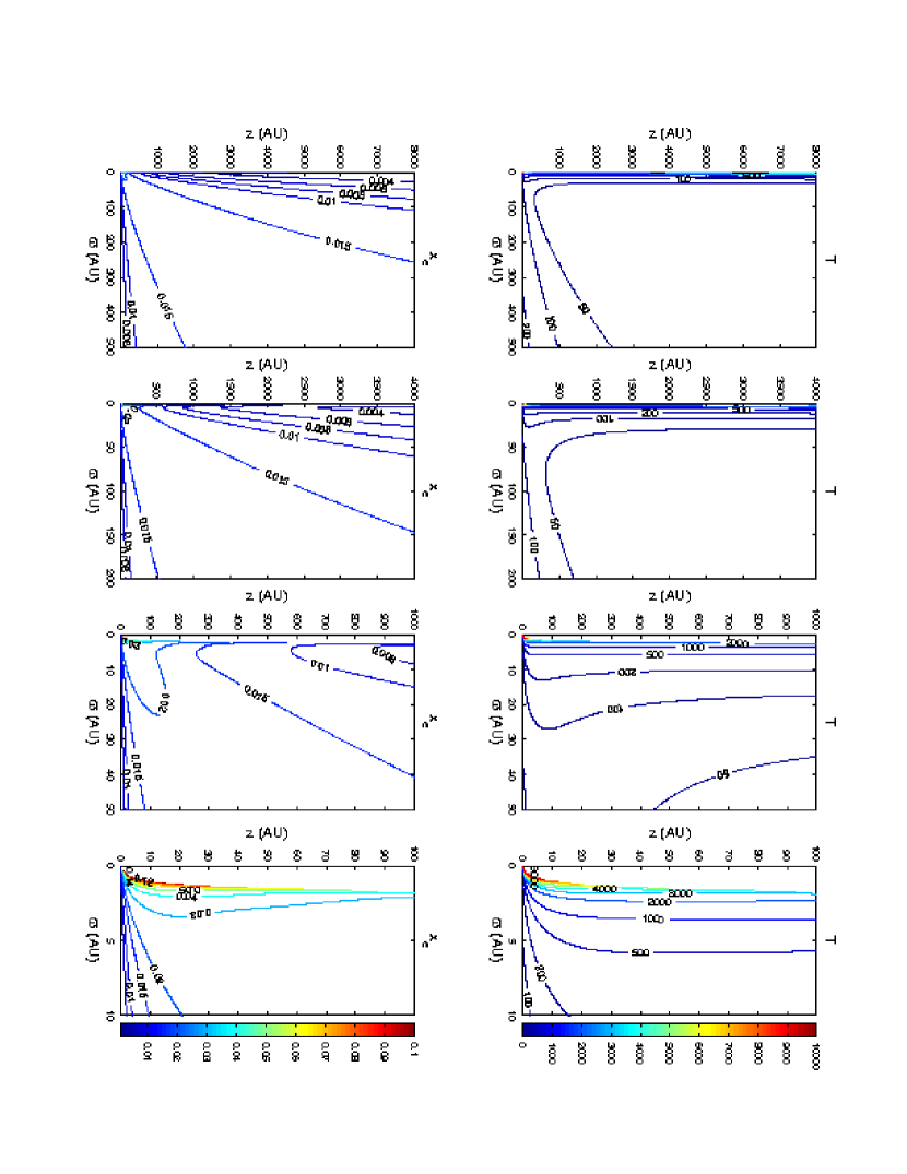
Figure 1: Temperature (upper) and ionization (lower) contours in the for the $\varpi-z$ plane for the fiducial case (defined in Table 2), but with $\alpha=0$ (no mechanical heating). The units for the spatial scales are AU. Note that the spatial scale proceeds from smaller to larger going from right to left.

In modeling the X-ray spectra of YSOs, we assume that a soft and a hard X-ray component are present with temperatures $kT_{\rm X}\approx 1$ keV and $kT_{\rm X}\approx 2-5$ keV, respectively. Since we focus on the more active YSOs that produce optical jets (and correspond to infrared classes I and II), we assume that the luminosities of the two components are the same order of magnitude, and that the total X-ray luminosity is substantially larger than the typical revealed Tauri star, e.g., $L_{\rm X}\approx 10^{31}$ erg s^-1. Of course $L_{\rm X}$ can be even higher during large flares (Feigelson & Montmerle 1999; Tsuboi 1999; Stelzer et al. 2000). As in the discussion of the hot spot radiation in §2.3, the calculation of the effects of the X-rays is complicated by the extended nature of the emitting regions and by the lack of relevant observational information on their physical properties. According to the x-wind model (see Fig. 1 of Shu et al. 1997), soft X-rays can be expected to arise within the region of closed stellar magnetic field lines (of linear dimension several $R_{\ast}$) and from the region above the funnel flow and beneath the helmet dome and kink point (of linear dimension $R_{\rm x}$). Hard as well as soft X-rays may be produced by reconnection events that occur either in the reconnection ring (in the equatorial plane from 0.75 $R_{\rm x}$ to $R_{\rm x}$) or along the helmet streamer above the kink point (at radial distances $\sim R_{\rm x}$). We deal with this complicated geometrical situation by representing the several finite sources by a set of axial point sources: half of both the soft and the hard X-rays are assumed to emanate from the origin and the other half from points displaced along the $z$-axis by $\pm 1.0R_{\rm x}$.

We follow the calculation by GNI of the X-ray ionization rate, which is based on the energy-smoothed cosmic photoelectric absorption cross section per H nucleus based on the compilation of Henke, Gullikson, and Davis (1993), similar to that used by Morrison and McCammon (1983),

$$\sigma_{\rm pe}(E)=\sigma_{\rm pe}(1\,{\rm keV})({\rm keV}/E)^{p};$$ (3-1)

for solar abundances, $p=2.485$ and $\sigma_{\rm pe}({\rm keV})=2.27\times 10^{-22}$ cm². We assume that moderate and high-energy X-rays are most important ($E\geq 1$ keV), and we ignore the relatively small contributions of the primary and Auger electrons compared to the dominant secondary electrons. We also assume that the electron fraction and the temperature are not high enough for the heavy atoms to be very ionized, so that the main X-rays absorbers are the K- and L-shells of heavy atoms. In other words, we approximate the production rate for primary photoelectrons as if the heavy atoms are in their ground states using equation (3-1). In the format of equation (2-13), the ionization rate due to the secondary electrons is

$${\cal P}_{\rm X}=\zeta=\frac{1}{4\pi r^{2}}\int_{E_{0}}^{\infty}\frac{L_{\rm X}(E)}{E}\sigma_{\rm pe}(E)\,e^{-\tau_{\rm X}}\,\left(\frac{E}{\epsilon_{\rm ion}}\right)dE\,,$$ (3-2)

where $L_{\rm X}(E)$ is the X-ray luminosity per unit energy interval, $\epsilon_{\rm ion}$ is the energy to make an ion pair (about 36 eV for an unionized hydrogen-helium mixture, according to Dalgarno, Yan, & Liu 1999), and $\tau_{\rm X}$ is the X-ray optical depth.

$$\tau_{x}\equiv\sigma_{\rm pe}(kT_{\rm X})N,\hskip 36.135ptN=\int_{0}^{r}n\,dr,$$ (3-3)

We introduce a low-energy cutoff $E_{0}$ because the smoothing used to obtain the power-law fit, equation (3-1), removes the thresholds in the underlying photoelectric cross sections. The smallest threshold is 0.0136 keV, but the operative cutoff may well be larger due to absorption in the source. Defining $\xi=E/kT_{\rm X}$, we choose $\xi_{0}=0.01$, e.g., $E_{0}=0.1$ keV for a thermal X-ray spectrum with $kT_{\rm X}=1$ keV because. Below this energy, the secondary electrons no longer dominate the ionization. We also need the X-ray heating rate,

$${\cal G}_{\rm X}=\frac{1}{4\pi r^{2}}\int_{E_{0}}^{\infty}\frac{L_{\rm X}(E)}{E}\sigma_{\rm pe}(E)\,e^{-\tau_{\rm X}}\,\left(y_{\rm heat}E\right)dE\,,$$ (3-4)

where $y_{\rm heat}$ is the fraction of the X-ray energy that heats the gas. Both $\epsilon_{\rm ion}$ and $y_{\rm heat}$ are functions of energy $E$ and electron fraction $x_{\rm e}$, the latter because of Coulomb scattering between the secondary and ambient electrons. We exploit the fact that, at energies much larger than characteristic atomic energies (measured by the ionization potential), $\epsilon_{\rm ion}$ and $y_{\rm heat}$ are approximately independent of energy. We can then extract the asymptotic factor $1/\epsilon_{\rm ion}$ from equation (3-2) and the asymptotic factor $y_{\rm heat}$ from equation (3-4). The result is that the direct X-ray heating, in the format of equation (2-12), can be expressed as

$${\cal G}_{\rm X}=y_{\rm heat}T_{\rm ion}\zeta,$$ (3-5)

where $T_{\rm ion}=\epsilon_{\rm ion}/k$. As discussed in Appendix B and §2.4.1, there is also an indirect X-ray heating term (Eq. [2-41]) that arises when the thermal effects of collisional excitation and de-excitation of the H atom are expressed in terms of Lyman-$\alpha$ cooling (Eq. [B12]).

The dependence of $\epsilon_{\rm ion}$ and $y_{\rm heat}$ on $x_{\rm e}$ has been studied by many authors, starting with Spitzer & Scott (1969) and most recently by Dalgarno, Yan, & Liu (1999), who give an extensive set of references to previous work. We have found that the parameterization of Shull & Van Steenburg (1983) for atomic H and He mixtures is useful in calculating the effects of X-rays on the inner x-wind with moderate mass-loss rates and not too large electron fractions. Their results are confirmed by Dalgarno et al. (1999) (who also provide the only theory for situations where the hydrogen is partly or fully molecular). According to Shull & Van Steenburg, the energy to make an ion pair can be written,

$${1\over\epsilon_{\rm ion}}={y_{\rm H}\over I({\rm H})}+{y_{\rm He}\over I({\rm He})},$$ (3-6)

where

$$y_{\rm H}=0.3908\,\left(1-x_{\rm e}^{0.4092}\right)^{1.7592},\qquad y_{\rm He}=0.0554\,\left(1-x_{\rm e}^{0.4614}\right)^{1.666},$$ (3-7)

and $I({\rm H})$ and $I({\rm He})$ are the ionization potentials of H and He. The heating fraction is

$$y_{\rm heat}=0.9971\,\left[1-\left(1-x_{\rm e}^{0.2663}\right)^{1.3163}\right].$$ (3-8)

It should be noted that existing theories of electron energy loss, on which our ionization and heating rates are based, do not hold much beyond $x_{\rm e}=0.1$. In particular, equation (3-5) breaks down in the limit $x_{\rm e}\to 1$, as can be seen from the behavior in this limit of equations (3-7) and (3-8). Fortunately, the maximum electron fractions encountered in the present calculations rarely exceed $x_{\rm e}=0.1$.

Putting all of this together for a thermal spectrum with temperature $T_{\rm X}$, the ionization rate at distance $r$ from an X-ray sources is,

$$\zeta\approx\zeta_{\rm x}\left({R_{\rm x}\over r}\right)^{2}\left({kT_{\rm X}\over\epsilon_{\rm ion}}\right)I_{p}(\tau_{\rm x},\xi_{0}),$$ (3-9)

where $\zeta_{\rm x}$ is the primary ionization rate at a distance $r=R_{\rm x}$. A useful numerical form for $\zeta_{\rm x}$ is

$$\zeta_{\rm x}\equiv{L_{\rm X}\sigma_{\rm pe}(kT_{x})\over 4\pi R_{\rm x}^{2}kT_{\rm X}}=1.13\times 10^{-8}{\rm s}^{-1}\left({L_{\rm X}\over 10^{30}{\rm erg}{\rm s}^{-1}}\right)\left({kT_{x}\over{\rm keV}}\right)^{-(p+1)}\left({10^{12}{\rm cm}\over R_{\rm x}}\right)^{2}.$$ (3-10)

The function $I_{p}(\tau_{\rm x},\xi_{0})$ in equation (3-9) describes the attenuation of the X-rays. As discussed by GNI, it decreases more rapidly with optical depth $\tau_{\rm x}$ than a power law at large optical depth and flattens out to a constant for very small optical depth. In the application to protoplanetary disks, the integral was evaluated numerically, but this is infeasible for detailed modeling of the x-wind. In Appendix C, we obtain an asymptotic form for $I_{p}(\tau_{\rm x},\xi_{0})$ using the method of steepest descents (as did Krolik & Kallmann 1983 and GNI) and then develop a simple interpolation method to combine the approximations for small and large optical depths.

4 Ambipolar Diffusion Heating

Long familiar from thermal considerations of interstellar clouds (Biermann & Schlüter 1950; Scalo 1977; Mouschovias 1978; Lizano & Shu 1987), the heating associated with ambipolar diffusion (e.g., Mestel & Spitzer 1956; Spitzer 1978; Shu II 1992) was first applied to protostellar winds by RGS and to disk winds by Safier (1993). Because RGS worked with a prescribed spherically-symmetric wind, they calculated the drag force of the ions on the neutrals from the wind equation of motion, i.e., as the net force of gravity plus acceleration. For T-Tauri stars with mass-loss rates in the range $10^{-8}-10^{-7}\,M_{\odot}$ yr^-1, RGS (Figure 9) obtained temperatures in the 4,000 — 5,000 K range within 10 $R_{\ast}$ but less than 100 K beyond $10^{4}R_{\ast}\approx 10^{16}$ cm (where the temperature decreases adiabatically as the 4/3 power of the distance). In this paper, we include ambipolar diffusion heating from first principles using the dynamical solution of Shang (1998) described in §2.1.

We use an improved approximation for the volumetric rate of ambipolar diffusion heating because, unlike the situation in interstellar clouds, the ionization level in the wind may not be very small:

$$\Gamma_{\rm AD}={\rho_{\rm n}|{\bf f}_{\rm L}|^{2}\over\gamma\rho_{\rm i}(\rho_{\rm n}+\rho_{\rm i})^{2}}.$$ (4-1)

Here $\rho_{\rm n}$ and $\rho_{\rm i}$ are the mass densities of the neutrals and the ions, respectively, ${\bf f}_{\rm L}$ is the Lorentz force,

$${\bf f}_{\rm L}=\frac{1}{4\pi}(\nabla\times{\bf B})\times{\bf B},$$ (4-2)

and $\gamma$ is the ion-neutral momentum transfer coefficient. A short derivation of equation (4-1) is given in Appendix D, based on the approximation that the difference in the acceleration (rather than the velocity) of the neutrals and ions can be ignored. When $\rho_{\rm i}<<\rho_{\rm n}$, equation (4-1) reduces to the usual one for low-ionization situations, e.g., Eq. (27.19) of Shu (II 1992). It has the important property that it does not become singular as $\rho_{\rm n}$ vanishes.

In Appendix E, we develop an improved formula for $\gamma$ that takes into account the latest calculations and experiments on the collision of ${\rm H}^{+}$ ions with atomic and molecular hydrogen and with helium, including exchange scattering in ${\rm H}^{+}$ + H collisions. For the case of no molecular hydrogen and $x_{\rm He}=0.1$, equation (E8) yields

$$\gamma=\frac{2.13\times 10^{14}}{1-0.714x_{\rm e}}\left[\{3.23+41.0T_{4}^{0.5}(1+1.338\times 10^{-3}\frac{w_{5}^{2}}{T_{4}})^{0.5}\}x({\rm H})+0.243\right]\\ \,{{\rm cm}^{3}{\rm s}^{-1}{\rm g}^{-1}},$$ (4-3)

where $T_{4}$ is the temperature in units of 10,000 K and $w_{5}$ is the slip speed (${\bf w}\equiv{\bf v_{\rm i}}-{\bf v_{\rm n}}$) in km s^-1. For temperatures approaching $10^{4}$ K, the new $\gamma$ is an order of magnitude larger than the value used by RGS and elsewhere in the literature. It agrees with Draine’s prescription (1980) only for cold clouds.

The slip velocity can be obtained from equation (D8) of Appendix D,

$${\bf w}={{\bf f}_{\rm L}\over\gamma\rho_{\rm i}(\rho_{\rm n}+\rho_{\rm i})}.$$ (4-4)

By eliminating $\gamma$ from the last two equations, we obtain a quartic equation for $w$, whose solution permits the coupling coefficient $\gamma$ to be calculated and then the ambipolar diffusion heating to be found from equation (4-1). The contribution from He to $\gamma$ in equation (4-3) (the last term) is always small.

A critical factor in the formula for ambipolar diffusion heating is the square of the Lorentz force (Eq. [4-2]). We calculate the Lorentz force by numerical interpolation on the global x-wind solution described in §2.1, which is itself an interpolation between an interior and an exterior (asymptotic) solution. Numerical experiments with different interpolation grids indicate that we have accurately calculated the Lorentz force for our approximate solution, but we do not have a good estimate of the error in the solution itself. However, it is reassuring that our calculations for a model close to that of RGS are consistent with their results.

Figure 1 shows the results for what we will call our fiducial model, defined in Table 2, except that the parameter $\alpha$ for mechanical heating (to be discussed in §5) has been set equal to zero. In other words, Figure 1 includes all of the processes listed in Table 1 except for mechanical heating. The upper panels show temperature contours and the lower panels ionization contours in the $\varpi$-$z$ plane. The spatial dimensions are AU and the scale of the plots increases from right to left. On the smallest scale (at the extreme right), the range in $\varpi$ is 10 AU and the range in $z$ is 100 AU. The temperature very close to the axis approaches 9,000 K, but the region hot enough to excite the forbidden lines, roughly $T>6,000-7,000$ K, occupies only a thin inner layer of the jet with a thickness less than 1 AU. The extreme right panel corresponds to an angular scale of less than $0.1^{\prime\prime}$ for objects at a distance of 150 pc, one not yet generally available to direct observation. The scale has begun to be explored by recent measurements with the Hubble Space Telescope (Bacciotti et al. 2000) and with an adaptive optics system on the Canada-Hawaii-France Telescope (Dougados, Cabrit, Lavalley, and Ménard 2000). On the commonly observed scales shown in the remaining panels of Figure 1, ranging from 1/3 to 3 arcsec, the wind is warm at best. The ionization fractions range from a few to 10%.

An analysis of the terms contributing to the basic ionization and heat equations, (2-13) and (2-12), reveals that a variety of processes contribute, especially close to the star. For example, the gas starting out on the last streamlines closest to the axis is ionized by both X-rays and by photoionization of the $n=2$ level and the negative ion of the H atom (by stellar and hot-spot radiation). The total ionization and recombination rates balance approximately at first, but, within a few AU, the ionization falls below the recombination rate and the electron fraction decreases slowly with distance (see section §6). For streamlines that start out at larger angles with respect to the axis, the X-rays are more important than stellar radiation for ionization. Because the density decreases more rapidly with distance along these streamlines, the ionization is essentially frozen into the streamline and decreases even more slowly with increasing distance.

Without mechanical heating, X-rays are generally the most important heating mechanism and adiabatic cooling the most important cooling mechanism. However, Lyman-$\alpha$ cooling is larger than adiabatic within the inner 10 AU, and ambipolar diffusion heating competes with X-rays at large distances beyond 500-1,000 AU. Because the thermal time scale is much shorter than the ionization time scale, the general dominance of adiabatic cooling over X-ray and ambipolar heating means that the temperature decreases rapidly on every streamline. Of course, as already noted, these heating mechanisms are relatively weak. It is perhaps not surprising that X-ray heating is not that effective, because only a small fraction of the system luminosity is in X-rays. In accord with equation (4-1), ambipolar diffusion heating is weak because the X-rays produce a relatively high level of ionization and because the coefficient $\gamma$ is an order of magnitude larger than used by previous workers. Much higher temperatures, along the lines obtained by Safier (1993) for disk winds, could be achieved without X-rays by using the conventional small (but incorrect) $\gamma$. For our objective of obtaining physical conditions that are compatible with the optical observations of jets, a wind thermal model based on stellar radiation, X-rays, and ambipolar diffusion heating is clearly inadequate.

5 Mechanical Heating

The previous section makes clear that neither heating by ambipolar diffusion nor heating by X-rays and the other radiation fields in the problem suffice to explain the observed emission lines of the abundant heavy elements in YSO winds and jets. We therefore consider whether a small fraction of the macroscopic flow energy in the x-wind can be tapped as a volumetric heat source. The physical basis for this idea resides in the observation that the actual flows are time-dependent (e.g., in the form of pulsed jets as discussed by Raga et al. 1990; Raga and Kofman 1992), with the time dependence generating shock waves or turbulent dissipation when fast fluid elements catch up with slower ones . We will not attempt a detailed discussion of the physics underlying the transformation of the fluctuating kinetic energy into heat (which might profitably be studied by 3-d numerical simulations); instead we appeal to general dimensional reasoning to parameterize the functional form of the mechanical heating.

The volumetric change in the kinetic energy of the flow is represented by the following terms in the fluid equations:

$${\partial\over\partial t}\left({\rho v^{2}\over 2}\right)+\nabla\cdot\left[\left({\rho v^{2}\over 2}\right){\bf v}\right]\equiv\Gamma_{\rm mech},$$ (5-1)

where $\rho$ and ${\bf v}$ are the local gas density and flow velocity in an inertial frame at rest with respect to the central star. Dimensional analysis suggests that we replace the above expression by

$$\Gamma_{\rm mech}=\alpha\,\rho\frac{v^{3}}{s}.$$ (5-2)

where $s$ is the distance the fluid element has traveled along a streamline to the location of interest in the wind, and where we have introduced a phenomenological coefficient $\alpha\geq 0$ to characterize the magnitude of the mechanical heating. A choice $\alpha\ll 1$ corresponds to the assumption that only a small fraction of the kinetic energy contained in the flow is dissipated into heat via shock waves and turbulent decay when integrated over the flow volumes of interest at the characteristic distances $s$ in the current problem.

The expression (5-2) could be made exact if we allowed $\alpha$ to be arbitrarily dependent on the spacetime coordinates $({\bf x},t)$. In practice, we shall make the simplifying assumption that $\alpha$ is a global constant, chosen to obtain a reasonable lighting up of the entire wind flow. With $\alpha\ll 1$, the scaling with $1/s$ in equation (5-2) could then be justified on the basis of the propagation of weak planar shocks where the velocity jump across the shock varies asymptotically as the inverse square root of the distance traveled (see §95 of Landau & Lifshitz 1959), with the energy deposited into heat (in the fixed frame) varying as the square of the velocity jump. In practice, we prefer to regard equation (5-2) not as being derived from specific dissipative processes, but as a generic model equation whose form satisfies broad physical considerations and whose utility comes from its simplicity of application within the context of small fluctuations about some mean time-steady flow.

From another perspective, when we remember that $v$ tends to $v_{\rm w}\approx 200-300$  km s^-1, it is clear that $\alpha$ must be much less than unity, for otherwise the wind will get too hot. We can roughly approximate adiabatic cooling by

$$\frac{3}{2}v(\frac{dT}{ds})_{\rm ad}\approx-\eta\frac{3}{2}\frac{vT}{s},$$ (5-3)

where $\eta$ is a parameter that is much less than one for streamlines close to the axis and of order unity at large angles ($\eta=1/3$ asymptotically, in the latter case). When this expression is balanced against the mechanical heating equation in (5-2), we obtain a rough estimate for the temperature

$$\frac{3}{2}kT\approx(\frac{\alpha}{\eta})mv^{2}.$$ (5-4)

From this result, we see that, not only is the collimated jet ($\eta\ll 1$) much hotter than the un-collimated wide-angle wind, but $\alpha$ must be much less than one in order to avoid heating the wide angle wind to extremely high temperatures. The full scale calculations discussed in §6 show that $\alpha\sim 10^{-3}$ yields jet temperatures in the $5,000-10,000$ K range that have been deduced from observations of forbidden lines.

6 Results

We now present the results of calculations for a fiducial or reference model, defined in Table 2, and for several variations on it.

Table 2. Fiducial Model
$M_{\ast}$	$0.8\,M_{\odot}$
$R_{\ast}$	$3.0\,R_{\odot}$
$R_{\rm x}$	$4.8\,R_{\ast}$
$2\pi/\Omega_{\rm x}$	7.5 d
${\dot{M}}_{\rm w}$	$3.2\times 10^{-8}\,M_{\odot}\,{\rm yr}^{-1}$
${\bar{v}}_{\rm w}$	195 km s-1
$L_{\ast}$	$2\,L_{\odot}$
$L_{\rm X}$	$4\times 10^{31}\,{\rm erg}\,{\rm s}^{-1}$
$\alpha$	$10^{-3}$

As remarked earlier, the parameters have been chosen to represent a solar-mass YSO in a fairly active phase. The numerical value of $L_{\rm X}$ pertains to two sources, one in and one above the reconnection ring, each with a soft and a hard component with individual X-ray powers of $10^{31}\,{\rm erg}\,{\rm s}^{-1}$. The parameter $\alpha$ has been chosen to have the order of magnitude $10^{-3}$ on the basis of an approximate solution for the temperature that includes only adiabatic cooling and mechanical heating and assumes that the density of a collimated streamline varies inversely with the distance.

6.1 Temperatures and Ionization Fractions

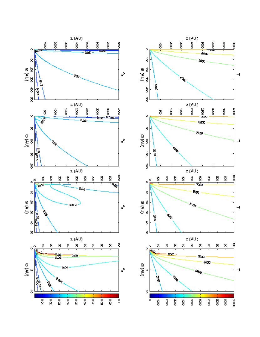
Figure 2: Temperature (upper) and ionization (lower) contours in the $\varpi-z$ plane for the fiducial case (defined in Table 2). The units for the spatial scales are AU.

Figure 2 shows the temperature and ionization profiles (contours of constant $T$ and $x_{\rm e}$) on various spatial scales in the same way as Figure 1 (for no mechanical heating). It is immediately clear from a comparison of the upper panels of Figures 1 and 2 that mechanical heating at this level leads to a much warmer wind. The electron fraction in the two sets of lower panels are not that different because X-rays dominate the ionization in both cases. The quantitative changes in $x_{\rm e}$ in going from Figure 1 to Figure 2 arise from several temperature-dependent ionization processes: recombination (decreases with increasing $T$), photodetachment of ${\rm H}^{-}$ (${\rm H}^{-}$ abundance increases with $T$), and photoionization of the $n=2$ level of atomic hydrogen (population increases with $T$).

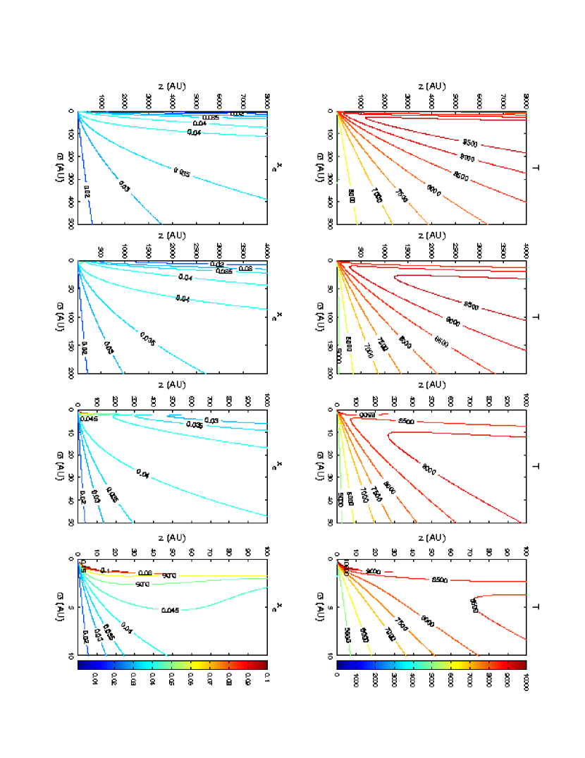
Figure 3: Temperature (upper) and ionization (lower) contours in the $\varpi-z$ plane for the fiducial case (defined in Table 2), but with $\alpha=0.002$. The units for the spatial scales are AU.

The wide range of physical properties manifested in the x-wind imply that many physical processes are important, although only a few will dominate at any particular location. For the fiducial model and modest variations on it, certain processes do play a more global role. For ionization, they are X-ray ionization and radiative recombination; for heating, X-rays and mechanical heating; and for cooling, Lyman-$\alpha$ and adiabatic cooling. We find that the relative contribution of a process varies from streamline to streamline and also with distance along an individual streamline. For example, photoionization of the $n=2$ level of atomic hydrogen is the most important ionization process within a few AU of the star for the last 10% of the streamlines close to the jet axis. X-rays then take over and are effective over distances of 10-20 AU for producing the initial ionization of these streamlines. At larger distances, the total ionization rate is smaller than the recombination rate. Since the recombination time scale is longer than the dynamical time scale, the ionization tends to get frozen into the wind and $x_{\rm e}$ decreases slowly with increasing distance, as shown in the lower left panels of Figures 1-3. This behavior has been found in several jets of young stars, e.g., Dougados et al. (2000), Lavalley-Fouquet, Cabrit, and Dougados (2000), Bacciotti, Eislöffel, and Ray (1999), and Bacciotti and Eislöffel (1999). For most of the streamlines, the X-rays are responsible for setting up the initial ionization of the flow. Similarly, the inner wind out to 10 AU is mainly heated by X-rays, but mechanical heating dominates most of the rest of the flow.

In addition to adiabatic and Lyman-$\alpha$ cooling, gas on the inner streamlines close to the source is cooled by several atomic hydrogen processes discussed in §2.4, mainly recombination and ${\rm H}^{-}$ cooling (equations [2-37] and equations [2-26], respectively). Within a short distance from the source, adiabatic and Lyman-$\alpha$ cooling take over and eventually adiabatic cooling dominates. The transition to adiabatic cooling occurs more rapidly for the lower streamlines. The cooling by the forbidden lines of O I and S II also contribute significantly on the inner, collimated streamlines, eventually dominating adiabatic for the inner 10% of the streamlines and becoming one-third as strong as adiabatic for the inner 25% of the streamlines. For most of the rest of the (uncollimated) wind, forbidden line cooling is unimportant.

Although the wind for the fiducial case (Figure 2) has an ionization fraction in the right range, it is not hot enough to emit the forbidden lines at the levels observed in the brightest jets. We can achieve the desired temperatures by increasing the coefficient $\alpha$ for mechanical heating. For example, Figure 3 shows the temperature and electron fraction profiles when $\alpha$ is increased by a factor of two to $2\times 10^{-3}$. The temperature is increased by almost a factor of two, and the electron fraction by about 20%.

6.2 Synthetic Images

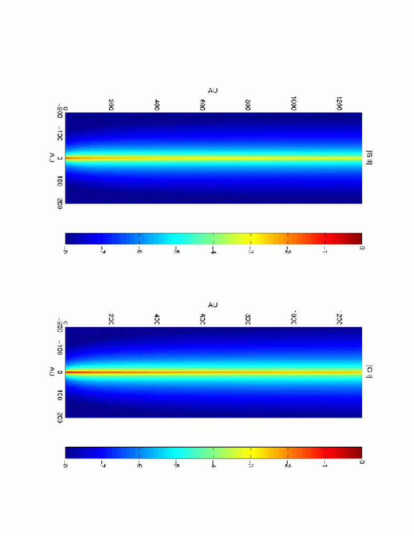
Figure 4: Synthetic images of the S II $\lambda$6731 (left) and O I $\lambda$6300 (right) brightness for the same model as in Figure 3 adapting the methods in SSG. The $\log_{10}$ of the integrated intensity is plotted in units of erg s^-1 cm^-2 ster^-1.

Figure 4 shows synthetic images of the wind in the forbidden lines of S II $\lambda$6731 (left) and O I $\lambda$6300 (right) for the case illustrated in Figure 3, as they might be observed edge-on and with near-perfect angular resolution. These images are similar to those constructed earlier by SSG, but with some unimportant technical differences in the way that we make the image of the innermost regions of the jet. The main physical difference with SSG is that here we calculate the temperature and electron fraction from an almost first-principles model, rather than assuming constant values for these parameters. The abundance of OI is calculated on the basis of a theory that gives the standard result given by Osterbrock (1989) for H II regions, i.e., O⁺ is maintained in chemical equilibrium by very fast forward and backward charge-exchange (assuming no H₂):

$$\frac{x({\rm O}^{+})}{x({\rm O})}=\frac{8}{9}\exp^{-227/T}\frac{x({\rm H}^{+})}{x({\rm H})}\approx\frac{8}{9}\exp^{-227/T}\frac{x_{\rm e}}{1-x_{\rm e}}.$$ (6-1)

The fact that ${\rm H}^{+}$ + O charge-exchange is fast means that O⁺ comes rapidly into equilibrium with the slowly-varying electron fraction. This situation does not generally hold for other atoms where charge exchange with ${\rm H}^{+}$ is much weaker, especially for sulfur. We are in the midst of developing a more general theory of the ionization of the major ionic carriers of jet forbidden lines. In the interim, we assume for Figure 4 that all of the sulfur is in S II (as in SSG).

We obtain the appearance of an optical jet in Figure 4 because the inner x-wind has a stratified density profile that varies approximately as the inverse square of $\varpi$ (SSG), the distance to the jet axis, and because the temperature and electron fraction have the right values to produce forbidden line emission. The base of the model jet in Figure 4 has a rounded conical shape suggestive of HST images (e.g., Eislöffel et al. 2000) and a horizontal width of the order of 25 AU. The width, which depends somewhat on definition, is determined by the critical density of the transitions, along with the temperature and electron fraction. The emissivities integrated along the line of sight decline very rapidly with horizontal distance from a cusp close to the axis. A careful inspection of the images near the equatorial plane reveals that O I $\lambda$6300 is stronger than S II $\lambda$6731, basically because high-temperature and high-density regions contribute more to the line-of-sight integral of the emissivity than the lower temperature and lower density regions that are more important at high altitudes. Here we are seeing the result of the competition between the lower critical density of the S II $\lambda$6731 transition and the greater intrinsic strength of the O I $\lambda$6300 transition (and larger O abundance). Images like Figure 4 provide a concrete basis for observational tests of our thermal-chemical theory of the x-wind jet.

6.3 Additional Parameter-Space Studies

In addition to the models shown in Figures 2-4, we have made some further exploratory calculations without attempting a systematic search of the model parameter space, defined largely by mass-loss rate ${\dot{M}}_{\rm w}$, X-ray luminosity $L_{\rm X}$, and mechanical heating strength $\alpha$. For example, we have calculated models with larger values of $\alpha$. Increasing $\alpha$ from 0.002 to 0.005 increases the temperature by about 2/3 and the electron fraction by about 1/3. Inside the jet ($\varpi\leq 25$ AU), $T$ is in the 10,000 - 13,000 K range and $x_{\rm e}$ is in the 0.03-0.05 range. This model may well have astrophysical applications, and its observational aspects will differ from those of the $\alpha=0.002$ model in Figures 3 and 4. For example, higher-excitation levels of O I and S II may be excited and significant abundances of O II and N II produced. An important question is whether a warm model, with $\alpha=0.005$ or larger, could produce a level of ionization sufficient to produce the forbidden lines by just collisional ionization of the H atom without X-rays. Setting $L_{\rm X}=0$ in the model with $\alpha=0.005$, we find that the electron fraction is reduced by about an order of magnitude and that the temperature is increased even further, e.g., up to 15,000 K inside the jet and even higher outside. (The decrease in $x_{\rm e}$ makes ambipolar diffusion heating effective close in and reduces some of the cooling). Obtaining wind ionization levels greater than a few percent by heating without X-rays doesn’t work without going to temperatures beyond the range indicated by the forbidden line observations. Some type of external mechanism is required to produce the degree of ionization inferred from observations, and we have shown that stellar X-rays are able to do the job.

When we examine the upper part of Figure 2, we see that the temperature of the wide-angle wind is quite high on the largest scale shown (the upper left panel), roughly between 3,000-6,000 K; for $\alpha=0.002$ (Figure 3) the range is 6,000-9,000 K. We are uncertain of the physical significance of this result because there are no measurements of the wind in this region (at least until larger distances are reached where the wind collides with ambient material). One possibility is that the mechanical heating formula used so far, equation (5-2), does not hold for the majority of the streamlines which are strongly divergent (where shockwaves do not propagate even approximately according to a planar description). Using other prescriptions (e.g., changing the density dependence in equation (5-2) from a linear to a nonlinear dependence), we find that the collimated jet can be made warmer and the uncollimated outer wind colder.

The total X-ray luminosity used in the fiducial model (Table 2), $L_{\rm X}=4\times 10^{31}\,{\rm erg}\,{\rm s}^{-1}$, is several times larger than the values determined by CHANDRA observations of young solar-mass YSOs in Orion (Feigelson 2001, private communication). However, the key physical parameter is the X-ray ionization parameter, $\zeta/n$, which determines the imprinting of the ionization at the base of the wind. Thus the essential model parameter is not $L_{\rm X}$ alone but something closer to $L_{\rm X}/{\dot{M}}_{\rm w}$, at least for small values of ${\dot{M}}_{\rm w}$ where X-ray absorption effects are small or moderate. We have run models for $\alpha=0.002$ (to match Figures 3 and 4) where $L_{\rm X}$ and ${\dot{M}}_{\rm w}$ are simultaneously decreased (and increased) by a factor 3. When $L_{\rm X}$ and ${\dot{M}}_{\rm w}$ are decreased by 3, the temperature is reduced slightly and the ionization fraction increased somewhat more due to the reduction in X-ray absorption. The net result is a model which is very similar to the ones shown in Figures 3 and 4. Increasing $L_{\rm X}$ and ${\dot{M}}_{\rm w}$ may also work, despite the fact that the electron factor is decreased by a factor of 2 because of the increase in X-ray absorption, simply because the emissivity of the forbidden lines is determined by the electron density rather than electron fraction. It should be recalled that $L_{\rm X}$ can also be greater than $10^{31}\,{\rm erg}\,{\rm s}^{-1}$ in flares and that changes in $L_{\rm X}$ and ${\dot{M}}_{\rm w}$ are likely to occur on different time scales.

The warm and ionized conditions found for the outer wind in Figures 1-3 are in stark contrast to the results of RGS because of our inclusion of X-ray ionization and mechanical heating in the present calculations. We have already discussed our uncertainty in applying the heating model of §5 to the uncollimated flow in the absence of compelling observational information about this part of the wind. It is quite possible that the wide-angle wind is not as warm as the above figures suggest. Furthermore, our thermal-chemical model needs to be extended in this region to include the thermal and chemical effects of molecules. Although not mentioned in §2, we have made a preliminary study of molecular hydrogen, mainly to insure that the abundance of ${\rm H}_{2}$ is negligible in the inner part of the wind. The molecular physics and heavy element chemistry of the wide-angle part of the wind are of considerable interest in connection with the detection of H₂ jets in young embedded YSOs (e.g., Zinnecker, McCaughrean, and Rayner 1998; Stanke, McCaughrean, and Zinnecker 1998), and we plan to return to this subject in the near future.

6.4 Line Ratios

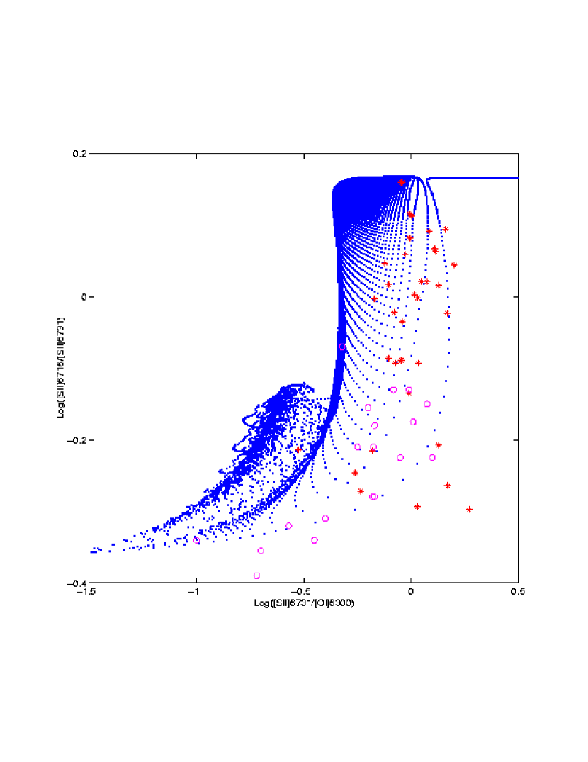
Figure 5: S II $\lambda$6716/S II $\lambda$6731 line ratio vs. the S II $\lambda$6731/O I $\lambda$ 6300 based on the synthetic images in Figure 4, where the jet is viewed perpendicular to its axis. The model parameters are given in Table 2 but with $\alpha=0.002$.

In addition to synthetic images of the forbidden line emission, like those displayed in Figure 4, we can also examine particular line ratios that are sensitive to the underlying physical properties of the wind as calculated in this paper. This approach has been widely used for H II regions and planetary nebulae (Osterbrock 1989), and it has been developed into a diagnostic tool for YSO jets by Bacciotti and Eislöffel (1999). Figure 5 is a plot of the S II$\lambda$6716/S II$\lambda$6731 line ratio vs. the S II$\lambda$6731/O I$\lambda$ 6300 line ratio based on the same model as the synthetic images in Figure 4, where the jet is viewed perpendicular to its axis. The former ratio (the ordinate in the figure) is diagnostic of $n_{\rm e}$ and the latter (the abscissa) is sensitive to $T$. The blue dots are the ratios formed from the line intensities for each pixel in the synthetic image of Figure 4, plotted one against the other. The dense concentration of blue points at the top of the “blue cliff” arise from distant wind locations with low temperature and electron density, whereas the points at the lower left come from close in where temperature and electron density are high. The red asterisks are data for HH objects from the compilation of Raga, Böhm, and Cantó (1996), and the red circles are data for DG Tau taken from Lavalley-Fouquet, Cabrit, and Dougados (2000). The comparison is meant to be illustrative and should not be taken too literally. The blue points have been obtained by “lighting up” every pixel of a steady-state jet, as modeled by a specific x-wind model with mechanical heating according to equation (5-2), and viewing the jet from a single direction. The asterisks are observations of a diverse set of HH objects viewed at a variety of angles and with a range of spatial resolution. Under these circumstances, we should not expect any more than a general kind of agreement.

The successful demarcation by the theory of the region in Figure 5 where observed YSO-jet line-ratios are found is therefore extremely satisfying. It confirms that the temperature and electron density (integrated along the line of sight) of our thermally and mechanically self-consistent x-wind model are indeed in the right range to explain the observations of real sources. It is significant that this agreement is obtained by adjusting the one free parameter at our disposal, $\alpha$, since the others are constrained by independent observations. We emphasize that we use the same value of $\alpha$ in the line-ratio plot of Figure 5 as in the image in Figure 4, $\alpha=0.002$. Lavalley-Fouquet et al. (2000) have attempted to correlate a similar data set with a complex shock model that employs a continuous distribution of shock velocities for each of 5 values of pre-shock density, ranging from $10^{2}-10^{6}$ cm^-3. The resulting line-ratio diagram then consists of a set of 5 curves or branches, one for each pre-shock density. Their analysis does not give the broad range of conditions observed for HH objects, but it is more successful with the more uniform set of high spatial-resolution data for DG Tau. The latter data appear to support a shock interpretation of the line ratios.

It is worth commenting that some of the extreme line-ratios, represented by the red circles in the lower left part of Figure 5, come from the highest spatial resolution measurements available for DG Tau obtained with adaptive optics (Lavalley-Fouquet et al. 2000). It is no coincidence, we believe, that the high temperature and electron-density conditions required to produce such ratios occur in the theoretical model near the base of the observed flow. By increasing the mass-loss rate slightly, these data would lie closer to the main body of the theoretical blue points in Figure 5. The observations of Lavalley-Fouquet et al. (2000) reinforce the importance of carrying out spectroscopic measurements at a spatial resolution sufficient to probe the extreme conditions close to the source of the jet. It is also noteworthy that the three red asterisks in the lower right of the diagram that fall outside the envelope of blue dots are all associated with strong bow shocks (Raga et al. 1996). The large jumps experienced across strong bow shock are evidently not well represented by the simple formula, equation (5-2), with a (weak-shock) value $\alpha=2\times 10^{-3}$. It should also not be too surprising that some data points lie outside of the theoretical range in Figure 5, considering that the blue dots have been calculated for a single viewing angle of one specific jet model, whereas the data sample a wide range of objects viewed under different conditions.

The main purpose of the line-ratio plot in Figure 5 is to ensure that the physical properties of the x-wind, as calculated in this paper, provide a sound foundation for quantitative comparisons between theory and observations. More detailed comparisons will require tailoring the theoretical models to the specific parameters of individual sources and considering additional diagnostics, e.g., the forbidden lines of other species and the radio continuum emission and radio recombination lines discussed in the next section. This next level of modeling would better constrain the adjustable parameters of the problem as well as test the theory under a wide range of flow and radiation conditions. Given the developments of this paper, such detailed tests are within our grasp, but their implementation is beyond the scope of the present paper.

7 Discussion

The results presented in §6 confirm that the thermal-chemical program described in this paper can provide the basis for making comparisons between x-wind theory and observations. Using the forbidden lines S II ($\lambda$6731) and O I ($\lambda$6300) from jets as the main example, we have shown that the collimated portion of the x-wind, when ionized by X-rays and heated mechanically, emits these lines in a manner strongly suggestive of the actual images made by observers (Figures 4). The model also appears capable of reproducing the measured line ratios (Figure 5). More definitive conclusions will require detailed quantitative comparisons between the theory and observations of individual objects. Thus we are in the midst of a study that considers further aspects of the forbidden lines, such as diagnostic line ratios of additional atoms and ions. The analysis of forbidden line images obtained at high spatial and spectral resolution have the potential to provide strong tests of the predictions that we are now able to make for the x-wind. In order to explore the jet structure predicted for scales smaller than 25 AU, observations with an angular resolution significantly better than $0.15^{\prime\prime}$ are required for sources at a distance of 150 pc. Recent measurements with the Hubble Space Telescope (Bacciotti et al. 2000) and with an adaptive optics system on the Canada-Hawaii-France Telescope (Dougados et al. 2000) have begun to probe jets on this scale.

An independent test of the x-wind model can be made by interferometric measurements of the radio continuum emission from the hot partially-ionized gas in the inner wind. Because of the absence of extinction, radio observations can probe deep into the inner wind close to the source of the outflow. Thermal radio emission has already been detected at the centers of more than 100 YSO outflows (Eislöffel et al. 2000; Rodríguez 1997), and about one fifth of these have been mapped at high spatial resolution, including a fair number that can be modeled to test the x-wind (Rodríguez 2001, private communication). According to the standard theory of thermal bremsstrahlung emission from a plasma with a uniform temperature (e.g., Shu I 1991), the optical depth is

$$\tau_{\rm ff}\approx 6\times 10^{-28}E\,{\rm cm}^{5}\,(\lambda/3{\rm cm})^{2}\,T_{4}^{-3/2},$$ (7-1)

where $T_{4}$ is the temperature in $10^{4}$ K and $E$ is the emission measure. In the approximation of Paper V, where the density at a given height above the midplane varies with horizontal distance as $\varpi^{-2}$, $\tau_{\rm ff}\propto\lambda^{2}\,\varpi^{-3}$, and the size of emission contours of a given intensity level should scale as $\lambda^{2/3}$, as observed in the best studied cases (see the review of Anglada 1996). Shorter wavelength observations are then favored for discriminating the wind from the cooler and lower density inner disk. We expect that the thermal bremsstrahlung emission for models with the fiducial parameters in Table 2 will be mainly optically thin, except very close to the source. We plan to synthesize the emission for models of the x-wind as it would be observed by the Very Large Array. If we are successful in reproducing the observations, we should be able to determine the mass-loss rates of thermal jets in a more realistic way than is currently done with the simple bi-conical model of Reynolds (1986).

Another way of testing the x-wind model with radio observations is provided by the mm and sub-mm recombination lines emitted by the hot plasma near the base of wind. Important kinematic information can be obtained by sensitive measurements of line shapes at high spatial resolution. High spectral resolution is also required to detect the lines in the presence of strong continuum emission by the disk at mm and sub-mm wavelengths. The hydrogen recombination lines that lie in the mm and sub-mm bands for $\alpha$ transitions ($n+1\rightarrow n$) occur for principal quantum numbers $n$ in the range 25-45. Welch and Marr (1987) made the first detection of mm recombination lines in the ultra-compact H II region W3(OH) with the H42$\alpha$ line at 86 GHz. This discovery was soon followed by other detections in regions of massive star formation (e.g., Gordon and Walmsley 1990) and by the discovery of masing transitions in MWC 349 by Martin-Pintado, Bachiller, Thum, and Walmsley (1989). Ground based and space observations of MWC 349 show that the masing reaches a broad peak at $n=19$ or 300 $\mu$m (Thum et al. 1998). To the best of our knowledge, radio recombination lines have not yet been detected in T Tauri stars. Rough preliminary estimates suggest that the radio recombination transitions produced in the x-wind will be weakly masing for lines that fall in the familiar sub-mm windows. We expect that some of these lines will be detected by new sub-mm instrumentation now under development such as the Sub Millimeter Array (SMA) and the Atacama Large Millimeter Array (ALMA). In order to calculate the emission and to synthesize images as observed with these new instruments, we need to supplement the program described in this paper with a full multi-level population calculation for hydrogen and with appropriate radiative transfer. These developments are now in progress, and we hope to report soon on the diagnostic prospects of the radio recombination lines for testing the validity of the x-wind model.

8 Conclusion

We have developed a thermal-chemical program that provides the basis for making detailed predictions for the x-wind model that can be compared with observations. The program incorporates new physical processes, particularly for heating (mechanical) and ionization (X-rays). The rate coefficients for all of the underlying microscopic processes have been re-evaluated and recalculated as required. In some cases, significantly different values have been obtained from those in the literature, e.g., the coefficient for ambipolar diffusion heating, and these should be useful in other problems.

In principle the program can describe a wide variety of flows, all within the context of the x-wind model. The key astrophysical model parameters are the mass-loss rate (${\dot{M}}_{\rm w}$), the X-ray luminosity ($L_{\rm X}$), and the mechanical heating strength ($\alpha$). The first two can be chosen to represent a particular kind of YSO at some stage of evolution, but a considerable range in these parameters is allowed by the observations. They may also be variable on short time scales, as is the case for the X-ray emission. In contrast, we regard $\alpha$ as a phenomenological parameter. For the case of an active but revealed source with an optical jet, the temperature of such jets, as seen in the forbidden lines of oxygen and sulfur, indicates that $\alpha\approx 2\times 10^{-3}$.

It is very likely that the three parameters, ${\dot{M}}_{\rm w}$, $L_{\rm X}$, and $\alpha$ are not all independent of one another. For example, we might expect that all three parameters decrease as we proceed from very young and active YSOs to older and less active ones. In this paper, we have concentrated on sources with optical jets to illustrate our approach. The exploration of other cases should lead to new opportunities for testing the x-wind model. In this context, an interesting question is what kinds of jets occur at earlier evolutionary stages when the mass-loss rate is much larger than we have used here, $\sim 3\times 10^{-8}\,M_{\odot}\,{\rm yr}^{-1}$. To answer this question, we are planning to extend the underlying physics of our model to include the essential molecular processes that are expected to occur when both the X-rays and the stellar radiation are more heavily extincted than in the cases treated in this paper.

The main result of this paper is the demonstration that the x-wind model, when extended to include thermal and chemical processes, has the capability to reproduce line ratios as well as images of the forbidden lines of jets in a self-consistent manner. We have also outlined a program for testing the model against the observations of individual objects, with the goal of better constraining the parameters of the problem and testing the theory under as wide a range of conditions as possible. The developments undertaken in the present paper now make such detailed tests possible.

Appendix A Rate Coefficient for ${\rm H}^{-}$-${\rm H}^{+}$ Neutralization

The exothermic channels of the reaction

$${\rm H}^{-}+{\rm H}^{+}\rightarrow{\rm H}(1)+{\rm H}(n)$$ (A1)

have the energy yields 12.582, 2.648, 0.758, and 0.096 eV for $n=1,2,3$ and 4. But curve-crossing considerations and detailed theoretical calculations (Fussen & Kubach 1986) indicate that, at mean center of mass energies less than 2 eV, reactions to the $n=3$ level dominate by a large margin over those to $n=2$.

The total neutralization cross section has been measured from 0.15-300 eV by Moseley, Aberth, & Peterson (1970), from 5-2000 eV by Szucs et al. (1984), and from 30-2000 eV by Peart, Bennett, & Dolder (1985). Only the lowest energies below a few eV are relevant for our astrophysical applications, and here the cross sections of Moseley et al. decrease with energy $E$ roughly as $E^{-1}$. However, the later experiments at higher energies clearly show that the results of Moseley et al. are too large by a factor of three. This conclusion is supported by the theoretical calculations of Fussen & Kubach (1986) with good potential energy curves.They give an analytic fit to the data below 3 eV (after renormalizing the low-energy results), from which we obtain the following approximation to the rate coefficient for ${\rm H}^{-}$-${\rm H}^{+}$ neutralization valid below 10,000 K:

$$k_{\pm}=\left[2.40\times 10^{-6}T^{-1/2}+4.96\times 10^{-9}+6.46\times 10^{-11}T^{1/2}+7.46\times 10^{-14}T\right]\,{\rm cm}^{3}{\rm s}^{-1}$$ (A2)

A typical value at $T=10,000$ K is $3.62\times 10^{-8}$cm³s^-1, which can be compared to the RGS value, $10^{-8}$cm³s^-1.

Appendix B Level Population of the Model Hydrogen Atom

We treat here the effects of collisional and X-ray ionization and excitation on the population of our model two-level ($n=1,2$) plus continuum ($c$) H atom. Table B lists the relevant processes and associated rates.

Table B. H Atom Processes
Collisional excitation and de-excitation	$C_{12},C_{21}$
Spontaneous decay	$A_{21}\beta_{21}$
Photoionization by the Balmer continuum	$g_{2c}$
Radiative recombination	$k_{\rm S}(\geq 2)$
Collisional ionization from $n=1,2$	$C_{1c}$, $C_{2c}$
X-Ray ionization from $n=1,2$	$\zeta_{1c}$, $\zeta_{2c}$
X-Ray excitation ($n=1$ to $n\geq 1$)	$\zeta_{12}$

The collisional rate coefficients have the form $C=x_{\rm e}nk(T)$ because we assume that electrons are the most important collision partners. We have used Voronov’s (1997) fit for $k_{1c}$; at $T=10^{4}$ K, it agrees to within 10% percent with the simpler formula used by RGS. For $k_{2c}$, we fit the rate coefficients given by Janev et al. (1987) to obtain

$$k_{2c}=7.37\times 10^{-10}T^{1/2}e^{-39,471{\rm K}/T}\,{\rm cm}^{3}\,{\rm s}^{-1}.$$ (B1)

For $T=10^{4}$ K, $k_{1c}$ is about $5\times 10^{-8}$ smaller than $k_{2c}$ so that, if the $n=2$ level is thermally populated, collisional ionizations from the $n=2$ level proceed at a faster rate than from the ground level. We use the same collisional de-excitation rate coefficient for the $n=2-1$ transition as RGS, based on Vernazza, Avrett, and Loeser (1981). The photoionization rate is given above in §2.4.1: $g_{2c}=W_{\ast}\,g_{{\rm A},\ast}(2)+W_{\rm h}\,g_{\rm A,h}(2)$ (Eq. [2-31]), as is the recombination rate, $k_{\rm S}(\geq 2)$ (Eq. [2-34]).

The X-ray rates in Table B are related to the rate $\zeta$ at which ion pairs are produced, discussed in §3. Because the cosmic X-ray absorption cross section in equation (3-1) is normalized to the abundance of hydrogen nuclei, the ionization rate per unit volume is $\zeta n$, where $n$ is the density of total hydrogen ($n_{\rm H}$), whereas the rates in Table B are defined in terms of level densities. In a H/He mixture, 88% of the X-ray produced ions are H⁺ ions (Dalgarno, Yan, & Liu 1999). If we ignore the small contribution from direct X-ray ionization of atoms in the $n=2$ level, then $0.88\zeta n=\zeta_{1c}n_{1}$. Using the approximate conservation relations, $n=n_{1}+n_{c}$ and $n_{\rm e}=n_{c}$, leads to $0.88\zeta n=\zeta_{1c}n(1-x_{\rm e})$, or

$$\zeta_{1c}=\frac{0.88}{1-x_{\rm e}}\zeta.$$ (B2)

Furthermore, for every H⁺ ion produced, 1.73 excited H atoms are produced (0.37 with $n>2$ (Dalgarno et al. 1999). Taking into account the radiative branching of these excited levels to $n=2$, the rate $\zeta_{12}$ is given by

$$\zeta_{12}=\frac{1.34}{1-x_{\rm e}}\zeta.$$ (B3)

The rate equations based on the processes in Table B are:

$$(\zeta_{12}+C_{12})n_{1}+x_{\rm e}nk_{\rm S}(\geq 2)n_{c}=(C_{21}+A_{21}\beta_{21}+g_{2c}+C_{2c}+\zeta_{2c})n_{2}$$ (B4)

$$x_{\rm e}nk_{\rm S}(\geq 2)n_{c}=(C_{1c}+\zeta_{1c})n_{1}+(g_{2c}+C_{2c}+\zeta_{2c})n_{2},$$ (B5)

$$n_{1}+n_{2}+n_{c}=n,\hskip 72.26999ptn_{c}=x_{\rm e}n.$$ (B6)

The ratio of the populations in the $n=1,2$ levels can be obtained by subtracting equation (B5) from equation (B4):

$$(C_{12}+C_{1c}+\zeta_{1c}+\zeta_{12})n_{1}=(C_{21}+A_{21}\beta_{21})n_{2},$$ (B7)

i.e. ,

$$\frac{n_{1}}{n_{2}}\equiv Q=\frac{k_{21}nx_{\rm e}+A_{21}\beta_{21}}{k_{12}nx_{\rm e}+k_{1c}nx_{\rm e}+\zeta_{1c}+\zeta_{12}}.$$ (B8)

The population of the $n=2$ level given in equation of §2.1.4 is obtained by ignoring $n_{2}$ in the conservation relation, equation (B6): $n_{1}\approx(1-x_{\rm e})n$. A quadratic equation for the steady electron fraction can also be obtained from equation (B5), but in this work we find $x_{\rm e}$ by integrating the rate equation (2-13). It may also be noted that recombination into and ionization processes out of the $n=2$ level drop out of the population ratio, $n_{1}/n_{2}=Q$.

The thermal implications of the above rate equations can be written as,

$$\Gamma-\Lambda=(n_{2}C_{21}-n_{1}C_{12})E_{21}+g_{2c}n_{2}\Delta E_{2c}-x_{\rm e}nk_{\rm S}(\geq 2)n_{c}kT-C_{1c}n_{1}I-C_{2c}n_{2}\Delta E_{2c}+\zeta_{1c}\Delta\epsilon_{1}n_{1},$$ (B9)

where $\Delta\epsilon_{1}$ is the X-ray heating energy when an ion pair is generated from the $n=1$ level, essentially the same as the heating energy used in §3, $\Delta\epsilon_{\rm heat}=y_{\rm heat}\Delta\epsilon_{\rm ion}$. When we use equation (B2) for $\zeta_{1c}$, the last term of equation (B9) becomes the usual X-ray heating term (and now includes He⁺), i.e.,

$$\Gamma-\Lambda=(n_{2}C_{21}-n_{1}C_{12})E_{21}+g_{2c}n_{2}\Delta E_{2c}-x_{\rm e}nk_{\rm S}(\geq 2)n_{c}kT-C_{1c}n_{1}I-C_{2c}n_{2}\Delta E_{2c}+\zeta n\Delta\epsilon_{\rm heat}.$$ (B10)

We can rearrange this result using population balance equation (B7),

$$(n_{2}C_{21}-n_{1}C_{12})E_{21}=-A_{21}\beta_{21}n_{2}E_{21}+(C_{1c}+\zeta_{1c}+\zeta_{12})E_{21}n_{1},$$ (B11)

so as to exhibit the conventional Lyman-$\alpha$ cooling:

$$\Gamma-\Lambda = -A_{21}\beta_{21}n_{2}E_{21}+g_{2c}n_{2}\Delta E_{2c}-x_{\rm e}nk_{\rm S}(\geq 2)n_{c}kT-\frac{1}{4}(C_{1c}n_{1}+C_{2c}n_{2})I$$ (B12)

$$+ \zeta n\left(\Delta\epsilon_{\rm heat}+2.22E_{21}\right).$$

We note that this form of the net heating has two X-ray terms, which we may refer to as direct and indirect heating. The direct term is the actual X-ray heating, e.g., as calculated by Shull & Van Steenburg (1983) and by Dalgarno, Yan, & Liu (1999), that arises from elastic collisions of (X-ray generated) electrons with the atoms and electrons of the partially ionized plasma. The indirect term, proportional to $E_{21}$, arises when the net thermal effect of collisional excitation and de-excitation is expressed in a form where the conventional Ly-$\alpha$ cooling appears. The large probability for inelastic scattering by secondary electron implies that the wind has a diffuse radiation field which we ignore for simplicity, except for trapped Ly-$\alpha$ radiation.

Appendix C X-ray Attenuation

The integral that appears in equation (3-9), $I_{p}(\tau_{x},\xi_{0})$, describes the attenuation of X-rays for a thermal spectrum (Krolik & Kallmann 1983),

$$I_{p}(\tau_{\rm X},\xi_{0})\equiv\int_{\xi_{0}}^{\infty}\xi^{-p}\exp\left[-\left(\xi+\tau_{\rm X}\xi^{-p}\right)\right]\,d\xi,$$ (C1)

where $\xi\equiv E/kT_{\rm X}$, $E_{0}$ is a low-energy cutoff, and the X-ray optical depth is given by

$$\tau_{\rm X}\equiv\sigma_{\rm pe}(kT_{\rm X})N,\qquad N=\int_{0}^{r}n\,dr.$$ (C2)

Following Krolik & Kallman (1983) and GNI, we use the method of steepest descents to derive the asymptotic formula

$$I_{p}\approx\left({2\pi\over p^{2}\tau_{\rm X}+\xi_{m}^{p+1}}\right)^{1/2}\xi_{m}^{-(p-2)/2}\exp[-(\xi_{m}+\tau_{\rm X}\xi_{m}^{-p})]\equiv J_{p}(\tau_{\rm X}),$$ (C3)

where $\xi_{m}$ satisfies the algebraic equation

$$\xi_{m}^{p}(p+\xi_{m})=p\tau_{\rm X},$$ (C4)

which we solve using Newton’s method with the initial guess $\xi_{m}=(p\tau_{\rm X})^{1/(p+1)}$. Derived for large $(p^{2}\tau_{\rm X}+\xi_{m}^{p+1})$, equation (C3) is accurate as long as $\xi_{m}>\xi_{0}$, i.e., even for $\tau_{\rm X}$ as small as

$$\tau_{0}\equiv{1\over p}\xi_{0}^{p}(p+\xi_{0})=3.4\times 10^{-3}$$ (C5)

when $\xi_{0}=0.1$. For $\tau_{\rm X}<\tau_{0}$, we derive the expansion (valid for $\xi_{0}\ll 1$) by repeated integration by parts:

$$I_{p}=\left\{{\xi_{0}\over(p-1)}-{[1-p\tau_{\rm X}\xi_{0}^{-(p+1)}]\xi_{0}^{2}\over(p-1)(p-2)}+\dots\right\}{\exp[-(\xi_{0}+\tau_{\rm X}\xi_{0}^{-p})]\over\xi_{0}^{p}}\equiv K_{p}(\tau_{\rm X},\xi_{0}).$$ (C6)

¿From equations (C3) and (C6), we construct the approximate fitting formula for all $\tau_{\rm X}$,

$$I_{p}(\tau_{\rm X},\xi_{0})=\left({\tau_{0}\over\tau_{0}+\tau_{\rm X}}\right)K_{p}(\tau_{\rm X},\xi_{0})+\left({\tau_{\rm X}\over\tau_{0}+\tau_{\rm X}}\right)J_{p}(\tau_{\rm X}).$$ (C7)

Appendix D Ambipolar Diffusion Heating for Large Ion Fractions

We analyze ambipolar diffusion heating with a two-fluid model for the ions and neutrals which satisfies the equations of motion

$$\rho_{\rm n}{\bf a}_{\rm n}=\rho_{\rm n}{\bf g}+{\bf f}_{\rm d},$$ (D1)

$$\rho_{\rm i}{\bf a}_{\rm i}=\rho_{\rm i}{\bf g}-{\bf f}_{\rm d}+{\bf f}_{\rm L},$$ (D2)

where

$${\bf a}\equiv({\bf v}\cdot\nabla){\bf v}$$ (D3)

stands for the steady-flow acceleration for in an inertial frame, ${\bf g}$ is the gravitational acceleration,

$${\bf f}_{\rm d}=\gamma\rho_{\rm n}\rho_{\rm i}({\bf v}_{\rm i}-{\bf v}_{\rm n})$$ (D4)

is the volumetric drag force of the ions on the neutrals, and ${\bf f}_{\rm L}=(\nabla\times{\bf B})f\times{\bf B}/4\pi$ is the volumetric Lorentz force. Addition of equations (D1) and (D2) yields the equation of motion for the combined ion-neutral fluid,

$$\rho{\bf a}=\rho{\bf g}+{\bf f}_{\rm L},$$ (D5)

where $\rho\equiv\rho_{\rm n}+\rho_{\rm i}$ is the total mass density (without the electrons) and ${\bf a}\equiv(\rho_{\rm n}{\bf a}_{\rm n}+\rho_{\rm i}{\bf a}_{\rm i})/\rho$ is the total acceleration.

The dynamics of the x-wind can be obtained to sufficient accuracy by ignoring the difference between ${\bf v}_{\rm n}$ and ${\bf v}_{\rm i}$ when we use equations (D3) and (D5) to compute the acceleration of the neutrals and the ions kinematically (from the mean velocity ${\bf v}\equiv(\rho_{\rm n}{\bf v}_{\rm n}+\rho_{\rm i}{\bf v}_{\rm i})/\rho$) and dynamically (from the total force $\rho{\bf g}+{\bf f}_{\rm L}$). We cannot ignore ${\bf v}_{\rm i}-{\bf v}_{\rm n}$ in the heating problem because ambipolar diffusion heating vanishes unless the ion and neutral velocities differ. However, we can use the equation for the difference in the accelerations obtained by subtracting $1/\rho_{\rm i}$ times equation (D2) from $1/\rho_{\rm n}$ times equation (D1):

$${\bf a}_{\rm n}-{\bf a}_{\rm i}=\left({1\over\rho_{\rm n}}+{1\over\rho_{\rm i}}\right){\bf f}_{\rm d}-{1\over\rho_{\rm i}}{\bf f}_{\rm L}.$$ (D6)

If we now ignore the difference in the accelerations, but not in the velocities, the left-hand side of D6 is zero and this equation yields

$${\bf f}_{\rm d}=\left({\rho_{\rm n}\over\rho_{\rm n}+\rho_{\rm i}}\right){\bf f}_{\rm L}.$$ (D7)

For lightly ionized media, $\rho_{\rm i}\ll\rho_{\rm n}$, we obtain ${\bf f}_{\rm d}={\bf f}_{\rm L}$. This is the expected and familiar result. When the ionization fraction is low, the ions have relatively little inertia and quickly reach terminal velocity governed by the balance of frictional and Lorentz forces, i.e., equation (D2) has the approximate solution, ${\bf f}_{\rm d}={\bf f}_{\rm L}$.

We now obtain the slip velocity from equation (D4) for the drag force,

$${\bf v}_{\rm i}-{\bf v}_{\rm n}={{\bf f}_{\rm L}\over\gamma\rho_{\rm i}(\rho_{\rm n}+\rho_{\rm i})}.$$ (D8)

This generalizes the lightly-ionized expression by replacing $\rho_{\rm n}$ in the denominator by $\rho_{\rm n}+\rho_{\rm i}$. Expression D8 is asymmetric in n and i because the Lorentz force acts only on charged particles. Thus, the slip velocity can become large if $\rho_{\rm i}$ becomes very small, but not if $\rho_{\rm n}$ becomes very small (when the sea of ions, moving under both gravity and the Lorentz force, simply drags the few neutrals that are present along with the rest of the almost completely ionized plasma).

The volumetric rate of heat input into the combined fluid by ambipolar diffusion is

$$\Gamma_{\rm AD}={\bf f}_{\rm d}\cdot({\bf v}_{\rm i}-{\bf v}_{\rm n}),$$ (D9)

and substitution of equations (D4) and (D8) leads to

$$\Gamma_{\rm AD}={\rho_{\rm n}|{\bf f}_{\rm L}|^{2}\over\gamma\rho_{\rm i}(\rho_{\rm n}+\rho_{\rm i})^{2}}.$$ (D10)

Notice that $\Gamma_{\rm AD}=0$ (instead of $\infty$) for a completely ionized plasma when $\rho_{\rm n}=0$ but $\rho_{\rm i}\neq 0$. Thus equation (D10) is self-limiting when $T$ approaches and exceeds $10^{4}$ K (and the gas becomes collisionally ionized. Although the treatment by Safier (1993) differs from ours, his $\Gamma_{\rm AD}$ also vanishes when $\rho_{\rm n}=0$.

Appendix E The Ion-Neutral Coupling Coefficient For Warm HI Regions

In order to calculate the ambipolar diffusion heating rate from D10, we need the momentum transfer rate coefficient $\gamma$ (dimensions cm³ s^-1 g^-1) introduced in equation (D4). The velocity field for each species consists of a mean velocity ${\bf v}$ plus a random velocity ${\bf u}$, which we assume is thermal. Each ion-neutral pair then gives a contribution to $\gamma$ which involves a double thermal average of the momentum transfer cross section and can be transformed into (Draine 1986):

$${\bf f}_{\rm d}=\gamma\rho_{\rm n}\rho_{\rm i}\,{\bf w}=\Sigma_{jk}n_{j}n_{k}m_{jk}\,{\bf w}_{jk}K_{jk}$$ (E1)

where $j$ and $k$ label ionic and neutral species, respectively, ${\bf w}\equiv{\bf v_{\rm i}}-{\bf v_{\rm n}}$, ${\bf w_{jk}}\equiv{\bf v_{j}}-{\bf v_{k}}$, $m_{jk}$ is the reduced mass,

$$K_{jk}=\frac{1}{\sqrt{\pi}}c_{jk}\,s_{jk}^{-3}\exp{(-s_{jk}^{2})}\int_{0}^{\infty}x^{2}\exp(-x^{2})\,[2xs_{jk}\cosh(2xs_{jk})-\sinh(2xs_{jk})]\,\sigma_{jk}(xc_{jk})\,dx,$$ (E2)

is a momentum transfer rate coefficient, $c_{jk}=\sqrt{2kT/m_{jk}}$, and $s_{jk}=w/c_{jk}$. We will approximate all of the ${\bf w}_{jk}$ by the slip speed ${\bf w}$ of the two-fluid model used in Appendix D and assume that the random velocities are all Maxwellian at the same kinetic temperature. When the momentum-transfer cross section varies inversely with the velocity, the integral reduces to the usual Langevin rate coefficient $v\sigma(v)$, whereas for a constant cross section it is (Draine 1986)

$$I=\frac{4}{3}\overline{v}\sigma\left[1+\frac{9}{16}(\frac{w}{\overline{v}})^{2}\right]^{1/2}$$ (E3)

where $\overline{v}=(8kT/\pi m)^{1/2}$ is the familiar mean relative velocity of a pair with reduced mass $m$. Before evaluating the sum in equation (E1), we discuss the cross sections that actually occur in this problem.

E.1 The Cross Sections

The model described in the main body of the text deals with warm atomic regions where the dominant ion is ${\rm H}^{+}$, in contrast to molecular clouds where heavy ions such as C⁺ and a variety of molecular ions (notably HCO⁺) are more important. The main collision partners of the ions are H and He atoms. Osterbrock (1961) focused on the central role of the (induced) polarization potential,

$$V=-\frac{1}{2}\alpha_{\rm pol}\frac{e^{2}}{r^{4}},$$ (E4)

in ion-neutral scattering, where $\alpha_{\rm pol}$ is the polarizability of the neutral; he calculated the rate coefficient for momentum transfer between a heavy interstellar-cloud ion and the dominant gas species, H, He, and H₂. Equation (E4) leads to a temperature-independent rate coefficient (Langevin-type, $\propto\alpha_{\rm pol}^{1/2}$). Following Draine (1980), essentially all authors have taken into account the breakdown of Osterbrock’s treatment at high temperatures, due to interactions of shorter range than $1/r^{4}$, by approximating their contribution by a constant cross section. In the case of Na⁺ + H₂ scattering, for example, Mouschovias & Paleologou (1981) (see also Draine, Roberge, & Dalgarno 1983) estimated this as a geometric cross section, $1.67\times 10^{-15}$ cm². This guess has not been borne out by the recent quantum calculations of Flower (2000), where the para-H₂-HCO⁺ cross section varies as $E^{-1/3}$ for energies between $10-10^{4}$ K, rather than the Langevin $E^{-1/2}$ dependence, although the numerical value of the rate coefficient at 20 K is essentially the Langevin value).

Draine (1980) also realized that H⁺+H scattering, basic to our calculations, is strongly affected by charge exchange because of the identity of the two nuclei. There are now good experiments of this reaction which provide a sound basis for the calculation of the momentum transfer rate coefficient. The definitive proof that charge transfer is significant comes from the merged beam experiment by Newman et al. (1982), which measures both H⁺ + H and H⁺ + D scattering with an ion optics system that can distinguish between charge exchange and elastic scattering down to energies as low as 0.1 eV. They obtain excellent agreement with the theory of Hunter & Kuriyan (1977), which is fully quantum mechanical and goes down to $10^{-4}$ eV and also agrees with the high-energy theory of Dalgarno & Yadav (1953) and other high-energy experiments (e.g., Gilbody 1994).

In addition to the definitive work of Hunter & Kuriyan (1977) for $E>10^{-4}$ eV, the momentum transfer cross sections have been calculated by Hodges & Breig (1991) in the same energy region, and by Krstić & Schultz (1998) for H⁺ + H, H⁺ + He, H⁺ + H₂ for energies $E>0.1$ eV. It is significant that, for none of the basic molecular ions (H${}_{2}^{+}$, HeH⁺, H${}_{3}^{+}$), does the scattering cross section manifest the pure $E^{-1/2}$ dependence of the Langevin theory. But when (diffraction) oscillations are averaged out, they all approximate this energy dependence below a certain energy $E_{1}$. The three cross sections behave differently above $E_{1}$, as seen in Table E1, which gives approximate power law fits to the momentum transfer cross section $\sigma_{\rm mt}(E)=\sigma_{\rm mt}(E_{1})(E/E_{1})^{p}$. The slopes below and above $E_{1}$ are $p_{1}$ and $p_{2}$, respectively.

Table E-1. Momentum Transfer Power Law Fits
System	$E_{1}$ (eV)	$\sigma_{\rm mt}(E_{1})$ 1	$p_{1}$	$p_{2}$
H+ + H	0.01	165	-1/2	-1/8
H+ + He	1.0	9.8	-1/2	-1
H+ + H2	5.0	5.6	-1/2	-2
1. Cross section units: $10^{-16}$ cm2

The break points $E_{1}$ are high enough for H₂ and He that the $E^{-1/2}$ fit is sufficient for $T<10^{4}$ K. For ${\rm H}^{+}$+H, however, both parts of the fit should be retained, although the high energy or exchange scattering dominates for $T>100$ K.

E.2 Calculations of the Rate Coefficient

When the momentum-transfer cross sections are approximated by high and low-energy power laws, as in Table E1, the rate coefficient in equation (E2) consists of two terms,

$$K=\alpha_{1}+\alpha_{2}.$$ (E5)

When we integrate over all energies for the first term, it becomes a constant, Langevin-type, rate coefficient, which we tabulate in Table E2.

Table E2. Rate Coefficients1
System	$\alpha_{1}$
H+ + H	3.23
H+ + He	1.52
H+ + H2	2.83
1. Units: $10^{-9}$ cm3  s-1

For H⁺ + H, we calculate $\alpha_{2}({\rm H})$ by replacing the $E^{-1/8}$ dependence in Table E1 by the (constant) average value for the interval $E=0.01-1.0$ eV ($1.5\times 10^{-14}$ cm²), integrating over all energy, and using Draine’s (1986) equation (E3). The result is

$$\alpha_{2}=4.10\times 10^{-8}{\rm cm}^{3}\,{\rm s}^{-1}\,T_{4}^{0.5}\,[1+1.338\times 10^{-3}\frac{w_{5}^{2}}{T_{4}}]^{1/2},$$ (E6)

where $T_{4}$ is the temperature in units of 10,000 K and $w_{5}$ is the drift speed in km s^-1. Notice that, for $T=10^{4}$ K, $\alpha_{2}(H)$ is more than an order of magnitude larger than $\alpha_{1}(H)$ due to the dominance of charge exchange scattering for $E>0.01$ eV.

For the temperature range of interest, $10^{2}<T,10^{4}$ K, ${\rm H}^{+}$ + H dominates over ${\rm H}^{+}$ + He and ${\rm H}^{+}+{\rm H}_{2}$ scattering because of abundance considerations and also because ${\rm H}^{+}$ + H scattering is so much stronger for $E>0.01$ eV. The high-energy contribution $\alpha_{2}$ can be ignored for ${\rm H}_{2}$ and He because the breakpoints $E_{1}$ are larger than for H and because the cross sections decrease more rapidly than the characteristic low-energy dependence on $1/v$. Thus $\alpha_{1}$ in Table E2 gives a good approximation (actually upper limit) to the momentum-transfer rate coefficients for ${\rm H}^{+}$ + He and ${\rm H}^{+}$ + ${\rm H}_{2}$ in the temperature region of interest

On substituting these results into equation (E1), we find that the ion-neutral coupling coefficient is

$$\gamma=\frac{1}{2m_{\rm H}}\frac{x({\rm H})[\alpha({\rm H})_{2}+\alpha({\rm H})_{2}]+(4/3)x({{\rm H}_{2}})\alpha({\rm H}_{2})_{1}+(8/5)x_{\rm He}\alpha({\rm He})_{1}}{x_{\rm H}+2x_{{\rm H}_{2}}+4x_{\rm He}},$$ (E7)

or, numerically,

$$\gamma = \left(\frac{2.13\times 10^{14}}{1-0.714x_{\rm e}}\right){{\rm cm}^{3}\;{\rm s}^{-1}\;{\rm g}^{-1}}$$ (E8)

$$\times \left[\{3.23+41.0T_{4}^{0.5}(1+1.338\times 10^{-3}\frac{w_{5}^{2}}{T_{4}})^{0.5}\}x({\rm H})+2.21x({{\rm H}_{2}})+2.43x_{\rm He}\right].$$

References

- (1) Anglada, G. 1996, in Radio Emission from the Stars and the Sun, eds. A. R. Taylor & J. M. Paredes, (PASP: San Francisco), 3
- (2) Bacciotti, F., Chiudere, C. & Oliva, T. 1995, A&A, 296, 185
- (3) Bacciotti, F. and Eislöffel, J. 1999, A&A, 342, 717
- (4) Bacciotti, F., Mundt, R., Ray, T.P., Eislöffel, J., Solf, J., & Camenzind, M. 2000, ApJ, 357, L49
- (5) Bacciotti, F. 2001, Rev. Mex. AA (Serie de Conferencias), in press
- (6) Biermann, L. & Sclüter, A. 1950, Zs. f. Naturf. 5a, 237
- (7) Black, J.H. 1987, Interstellar Processes, eds. D. J. Hollenbach and H. A. Thronson, Jr., (Dordrecht: Reidel), 731-744.
- (8) Calvet, N. & Gullbring, E. 1998, ApJ, 509, 802
- (9) Dalgarno, A., Yan, M., & Liu, W.-H. 1999, ApJS, 125, 237
- (10) Dalgarno, A. & Yadav, H.N. 1953, Proc. Roy. Soc., A66, 173
- (11) Dougados, C., Cabrit, S., Lavalley, C., & Ménard, F. 2000, A&A, 357, L61
- (12) Draine, B. T., 1980, ApJ, 241, 1021
- (13) Draine, B. T., 1986, MNRAS, 220, 133
- (14) Draine, B. T., Roberge, W.G., & Dalgarno, A. 1983, ApJ, 264, 485
- (15) Eislöffel, J., Mundt, R., Ray, T. P., Rodríguez, L. F. 2000, in Protostars and Planets IV, eds. V. Mannings, A.P. Boss, and S. Russell, (Tucson: University of Arizona Press), 815
- (16) Feigelson E.D. & Montmerle, T. 1999, ARA&A, 37, 363
- (17) Flower, D.R. 2000, MNRAS, 313, L19
- (18) Fussen, D. & Kubach, C. 1986, J. Phys. B, 19, L31
- (19) Garmire, G., Feigelson, E.D., Broos, P., Hillenbrand, L.A., Pravdo, S.H., Townsley, L., & Tsuboi, Y. 200, AJ, 120, 1426
- (20) Glassgold, A.E., Mamon, G.A., & Huggins, P.J. 1991, ApJ, 373, 254
- (21) Glassgold, A.E., Najita, J. & Igea, J. 1997 (henceforth GNI), ApJ, 480, 344
- (22) Gilbody, H.B. 1994, Advances in Atomic, Molecular, and Optical Physics, 33,149
- (23) Gounelle, M., Shu, F.H., Shang, H., Glassgold, A.E., Rehm, K.E., & Lee, T. 2001, ApJ, 548, 1051
- (24) Gullbring, E., Calvet, N., Muzerolle, J., & Hartmann, L. 2000, ApJ, 544, 927
- (25) Hartigan, P., Bally. J., Reipurth, B., & Morse, J.A. 2000, in Protostars and Planets IV, eds. V. Mannings, A.P. Boss, and S. Russell, (Tucson: University of Arizona Press), 841
- (26) Henke, B.L., Gullikson, E.M., & Davis, J.C. 1993, At. Data Nuc. Data, Tables, 54, 181
- (27) Hodges, X. & Breig, Y. 1991, JGR, 96, 7697
- (28) Hunter, X. & Kuriyan, Y. 1977, Proc. Roy. Soc., A353, 575
- (29) Igea, J. & Glassgold, A.E. 1999, ApJ, 518, 848
- (30) Janev, R. K., Langer, W. D., & Evans, K. 1987, Elementary Processes in H-He Plasmas, (New York: Springer)
- (31) Johns-Krull, C. & Valenti, J.A. 2000, in Stellar Clusters and Associations: Convection, Rotation, and Dynamos, eds. R. Pallavicini, G. Micela, and S. Sciortino, (San Francisco: PASP), 371
- (32) Königl, A. & Ruden, S.P. 1993, in Protostars and Planets III, eds. E.H. Levy and J.I. Lunine 1993, (Tucson: University of Arizona Press), 641
- (33) Königl, A. & Pudritz, R.E, 2000, in Protostars and Planets IV, eds. V. Mannings, A.P. Boss, and S. Russell, (Tucson: University of Arizona Press), 759
- (34) Koyama, K. in Star Formation 1999, ed. T. Nakamoto (Nobeyama: Nobeyama Radio Obs.), 269
- (35) Krstić, P.S. and Schultz, D.R.1998, Atomic and Plasma-Material Data for Fusion 8, 1
- (36) Krolik, J. H. & Kallmann, T. R. 1983, ApJ, 267, 610
- (37) Landau, L. D. & Lifshitz, E. M. 1959, Fluid Mechanics, (London: Pergamon Press)
- (38) Lvalley-Fouquet, C., Cabrit, S., and Dougados, C. 2000, A&A, 336, L41
- (39) Lee, T., Shu, F. H., Shang, H., Glassgold, A. E., Rehm, K. E. 1998, ApJ, 506, 898
- (40) Lizano, S. & Shu, F.H. 1987, in NATO/ASI Physical Processes in Interstellar Clouds, ed. M. Scholer (Dordrecht: Reidel), 173
- (41) Gordon, M.A. & Walmsley, C.M. 1990, ApJ, 365, 606
- (42) Martín-Pintado, J., Bachiller, R., Thum, C., & Walmsley, C. M. 1989, A&A, 215, L13
- (43) McKee, C.F. & Zweibel, E. 1995, ApJ, 440, 686
- (44) Mestel, L. & Spitzer, L. Jr., 1956, MNRAS, 116, 50
- (45) Milalas, D. 1970, Stellar Atmospheres (San Francisco: W.H. Freeman)
- (46) Mohanty, S. & Shu, F. H. 2001, ApJ, in preparation
- (47) Morrison, R. & McCammon, D. 1983, ApJ, 270, 119
- (48) Moseley, J., Aberth, W., & Peterson, J.R. 1970, Phys. Rev. Lett.,24, 435
- (49) Mouschovias, T. Ch. 1978, in Protostars and Planets, ed. T. Gehrels, (Tucson: University of Arizona Press), 209
- (50) Mouschovias, T. Ch & Paleologou, E. V. 1981, ApJ, 246, 48
- (51) Najita, J, & Shu, F.H. 1994, ApJ, 429, 808 (Paper III)
- (52) Newman, J.H., Cogan, J.D., Ziegler, D.L., Nitz, D.E., Rundel. R.E., Smith, K.A., & Stebbings, R.F. 1982, Phys. Rev. A25, 2976
- (53) Osterbrock 1961, ApJ, 134, 270
- (54) Osterbrock 1989, Astrophysics of Gaseous Nebulae and Active Galactic Nuclei, (Mill Valley: University Science)
- (55) Ostriker, E. C., Gammie, C. F., & Stone, J. M. 1999, ApJ, 513
- (56) Ostriker, E. & Shu, F.H. 1995, ApJ, 447, 813 (Paper IV)
- (57) Peart, B., Bennett, M.A., & Dolder, K. 1985, J. Phys. B18, L439
- (58) Peres, G., Orlanda, S., Reale, F., Rosner, R., & Hudson, H. 2000, ApJ, 528, 537
- (59) Raga, A. C., Cantò, J., Binette, L., and Calvet, N. 1990, ApJ, 364, 601
- (60) Raga, A. C. and Kofman, L. 1992, ApJ, 386, 222
- (61) Raga, A. C., Böhm, K.-H., Cantò, J. 1996, Rev. Mex. Astron. Astrofis. , 32, 161
- (62) Rodríguez, L. F. 1997, in Herbig-Haro Flows and the Birth of Low Mass Stars, IAU Symposium No. 182, eds. B. Reipurth and C. Bertout (Dordrecht: Kluwer), 83
- (63) Rodríguez-Fernández, N.J., Martín-Pintado, J., Fuente, A., de Vincente, P., Wilson, T.L., Hüttmeister, S. 2001, A&A, 365, 174
- (64) Reynolds, S.P. 1986, ApJ, 304, 713
- (65) Ruden, S.P., Glassgold, A.E., & Shu, F.H. 1990, ApJ, 361, 546 (henceforth RGS)
- (66) Safier, P. 1993, ApJ, 408, 115
- (67) Seaton, M. J. 1964, MNRAS, 127, 177
- (68) Scalo, J. M. 1977, ApJ, 2113, 705
- (69) Schmitt, J. H. M. M., Collura, A., Sciortino, S., Vaiaba, G. S., Harnden, F. R., Jr, & Rosner, R. 1990, ApJ, 365, 704
- (70) Szucs, S., Karemera, M., Terao, M., and Brouillard, F. 1984, J. Phys. B17, 1613, 1984
- (71) Shang, H. 1998, Ph. D. thesis, University of California at Berkeley
- (72) Shang, H., Shu, F.H., & Glassgold, A.E. 1998, ApJ, 493, L91
- (73) Shu, F. H., Ruden, S. P., Lada, C. J., & Lizano, S. 1991, ApJ, 370, L31
- (74) Shu, F.H. 1991, The Physics of Astrophysics, Vol. I, Radiation, (Mill Valley: University Science Books)
- (75) Shu, F.H. 1992, The Physics of Astrophysics, Vol. II, Gas Dynamics, (Mill Valley: University Science Books)
- (76) Shu, F.H., Najita, J., Ostriker, E. C., Wilkin, F., Ruden, S., & Lizano, S. 1994a, ApJ, 429, 781 (Paper I)
- (77) Shu, F.H., Najita, J., Ruden, S., & Lizano, S. 1994b, ApJ, 429, 797 (Paper II)
- (78) Shu, F.H., Najita, J., Ostriker, E. C., & Shang, H. 1995, ApJ, 455, L55 (Paper V)
- (79) Shu, F.H., Shang, H., Glassgold, A. E., & Lee, T 1997, Science, 277, 1475
- (80) Shu, F.H., Najita, J.R., Shang, H., & Li, Z.-Y. 2000, in Protostars and Planets IV, eds. V. Mannings, A.P. Boss, and S. Russell, (Tucson: University of Arizona Press), 789
- (81) Shull, M. & Van Steenburg, M.E. 1983, ApJ, 298, 268
- (82) Skinner, S. L. & Walter, F. M. 1998, ApJ, 509, 761
- (83) Spitzer, L. Jr. & Scott, E. H. 1969, ApJ, 158, 161
- (84) Spitzer, L., Jr. 1978, Physical Processes in the Interstellar Medium, (New York: Wiley-Interscience)
- (85) Stancil, P. C., Lepp, S., & Dalgarno, A. 1998, ApJ, 509, 1
- (86) Stanke, T., McCaughrean, M. J., & Zinnecker, H. 1998, A&A, 332, 307
- (87) Stelzer, B., Neuhäuser, R., & Hambaryan, V. 2000, A&A, 356, 949
- (88) Thum, C., Martín-Pintado, J., Quirrenbach, A., & Matthews, H.E., A&A, 333, L63
- (89) Tsuboi, Y. 1999, Ph.D. thesis, Kyoto Univ.
- (90) Vernazza, J.E., Avrett, E.H., & Loeser, R. 1981, ApJS, 45, 635
- (91) Verner, E.M., Verner, D.A., Korista, K.T., Ferguson, J.W., Hamann, F., & Ferland, G.J. 1999 ApJS, 120, 101
- (92) Verner, E.M., Verner, D.A., Balwin, J.A., Ferland, G.J., amd Martin, P.G. 2000, ApJ, 543, 831
- (93) Voronov, G.S. 1997, ADNDT, 65, 1
- (94) Welch, W.J., Jr. & Marr, J. 1987, ApJ, 317, L21
- (95) Wishart, A. W. 1979, MNRAS, 187, 59
- (96) Woitke, P. & Sedlmayr, E., 1999, A&A, 347, 617
- (97) Zinnecker, H., McCaughrean, M.J., & Rayner, J., 1998, Nature, 394, 862