Non-iterative methods to estimate the in-flight noise properties of CMB detectors

We present a new approach for statistical inference on noise properties of CMB anisotropy data. We consider a Maximum Likelihood parametric estimator to recover the full dependence structure of the noise process. We also consider a semiparametric procedure which is only sensitive to the low frequency behavior of the noise spectral density. Both approaches are statistically robust and computationally convenient in the case of long memory noise, even under nonstationary circumstances. We show that noise properties can be consistently derived by such procedures without resorting to currently used iterative noise-signal methods. More importantly, we show that optimal (GLS) CMB maps can be obtained from the observed timestream with the only knowledge of the noise memory parameter, the outcome of our estimators.

1 Introduction

Recent high sensitivity, high resolution observations of the Cosmic Microwave Background (CMB) anisotropy are posing strong constraints on Cosmology (see, e.g., Balbi et al., 2000; de Bernardis et al., 2001). The ability to discriminate among different cosmological scenarios critically relies on the efficiency and accuracy of the data analysis pipeline, other than -obviously- on experimental know-how. In order to be efficient, data analysis has to deal with the size of the data sets, which is bound to increase with new space missions such as MAP and Planck Surveyor. In order to be accurate, the data analysis pipeline should implement optimal statistical techniques to reconstruct the correlation structure of receiver noise, i.e. the behavior of its spectral density. This is a critical point for data analysis of CMB anisotropy one-horned experiment. In fact, both Maximum Likelihood map making (see e.g. Wright, 1996; Borrill, 1999; Natoli et al., 2001) and angular power spectrum estimation (Tegmark 1997; Bond et al., 1998; Oh et al., 1999) heavily depend on the knowledge of the noise spectral density, which of course must be determined from the data themselves.

Our paper is not the first to focus on estimating the noise properties out of a CMB anisotropy data stream. Ferreira & Jaffe (2000) advocated simultaneous estimation of signal and noise on the basis of a Bayesian approach. However, their estimates for the noise spectral density are piecewise constant with several discontinuities. Far from being realistic, this assumption does not apply to long range dependence models. Prunet et al. (2001) obtained a purely nonparametric estimate of the noise spectral density as a by-product of their iterative map making procedure. Even if cast in a frequentist framework, the resulting algorithm is very similar to Ferreira and Jaffe’s proposal. It is worth noting that, in both cases, purely nonparametric estimates of noise properties lack a rigorous justification in the statistical literature if noise is a long memory process. In this case, all of these difficulties can be overcome by using well known and robust statistical techniques which are well supported by the most recent literature (Fox & Taqqu, 1986; Dahlhaus, 1995; Robinson 1995ab; Giraitis & Taqqu, 1999). In Sect. 2 we discuss these techniques in the context of CMB data analysis. In Sect. 3 we apply them to simulated datasets of the Planck and BOOOMERanG experiments. Finally, in Sect. 4 we draw our main conclusions and point out directions for future research.

2 Efficient estimation of the noise properties

We assume that the data, ${\bf d}$, consist of the sum of two uncorrelated time series:

$$d_{t}=s_{t}+n_{t}$$ (1)

for $t=1,2,\dots,T$. Here ${\bf n}$ and ${\bf s}$ are noise and signal, respectively. The latter is modeled assuming linear dependence on the sky pattern:

$$s_{t}=\sum_{p=1}^{K}P_{tp}m_{p}.$$ (2)

We imagine the “map” ${\bf m}$ to be smeared by the instrumental beam and discretized into $K$ elements (or pixels). The matrix ${\bf P}$ effectively defines the experimental scanning strategy by “unrolling” the sky map into a time series. We limit ourselves to the case of one-horned experiments and symmetric beam profile, for which the matrix ${\bf P}$ has a very simple structure, consisting of a single non zero entry (with value $1$) per row. This entry corresponds to the pixel observed at a given time $t$. For very low signal to noise (S/N) ratio the timestream, ${\bf d}$, is noise dominated. In this Section we pretend that this is the case. We will show below, in Sect. 3, how to drop this assumption.

2.1 Long memory processes

A process is said to be wide sense (or second order) stationary if its mean, variance and covariance functions are finite and constant over time: $\langle n_{t}\rangle=\mu$, $\langle n_{t}n_{t}\rangle=\gamma(0)<\infty$ and $\langle n_{t}n_{t-\tau}\rangle=\gamma(\tau)$, $\tau=\pm 1,\pm 2,\dots$. For a noise process we shall take $\mu\equiv 0$. The Cramér Representation Theorem ensures that for any second order stationary process we can write:

$$n_{t}=\int_{-\pi}^{\pi}\exp(itf)\sqrt{P(f)}\,dW(f)\,,$$ (3)

where $W(f)$ is a random measure such that $\langle dW(f)\rangle=0$, while $\langle dW(f)dW(g)\rangle=df$ if $f=g$ and $0$ otherwise (i.e. $W$ represents a white noise measure). The function $P(f)$ is the spectral density function of the process ${\bf n}$, uniquely related to the sequence of covariances $\gamma(\tau)$ through the usual Fourier formulae:

$$P(f) = \frac{1}{2\pi}\sum_{\tau=-\infty}^{\infty}\gamma(\tau)\exp(-i\tau f)\text{ , }$$

$$\gamma(\tau) = \int_{-\pi}^{\pi}\exp(-i\tau f)P(f)df\text{ .}$$

Thus, wide sense stationarity implies:

$$\gamma(0)=\int_{-\pi}^{\pi}P(f)df<\infty\text{ ,}$$

that is, the spectral density needs always be integrable. State of the art microwave detectors produce “$1/f$” noise. We shall therefore focus on long memory (or long range dependent) noise. For this processes the spectral density is such that

$$\lim_{f\rightarrow 0}\frac{P(f)}{f^{-\alpha}}=G,$$ (4)

where $0<G<\infty$ and $0<\alpha<1$. So, even if divergent at zero frequency, the spectral density is always integrable. Eq. (3) can be discretized as follows:

$$n_{t}=\frac{1}{\sqrt{2\pi T}}\sum_{j=1}^{T}\exp(itf_{j})\sqrt{P(f_{j})}\;\varepsilon_{j},$$ (5)

Here $f_{j}=2\pi j/T$ are Fourier frequencies, while $\varepsilon_{j}$ denotes a sequence of zero-mean, independent and identically distributed ($i.i.d.$) variables with unit variance. Eq. (5) is widely used to generate random processes with a given spectral density $P(f)$ in Monte Carlo procedures. If we take, for instance, $P(f)=Gf^{-\alpha}$, straightforward algebra shows that:

$$\lim_{T\rightarrow\infty}\langle n_{t}n_{t}\rangle\simeq\lim_{T\rightarrow\infty}\frac{1}{2\pi T}\sum_{j=1}^{T}P(f_{j})=\left\{\begin{array}[]{c}O(1),\text{ }\alpha<1\\ O(\log T),\text{ }\alpha=1\\ O(T^{\alpha-1}),\text{ }\alpha>1\end{array}\right..$$

Therefore, if $\alpha\geq 1$ the variance of ${\bf n}$ grows with time, i.e. the process is not stationary. We shall first focus on the stationary case $\alpha<1$. This assumption will be relaxed to $\alpha<2$ in Sect. 2.4.

2.2 Fully parametric procedures

Assume first that the the functional form of the spectral density for the process ${\bf n}$ is known and completely specified by a set of parameters ${\bf\theta}\equiv(\theta_{1},\theta_{2},\dots,\theta_{N})$. For “$1/f$” noise it is customary to write:

$$P(f,{\bf\theta})=A\left\{1+\left(\frac{f_{k}}{f}\right)^{\alpha}\right\}$$ (6)

$\theta=(A,\alpha,f_{k})$, where $A$ is an amplitude, $f_{k}$ is the so-called knee frequency and $\alpha$ is the spectral index introduced above. Throughout this paper we shall assume that ${\bf n}$ is Gaussian even if this condition is not essential for our conclusions to hold. Under Gaussianity ${\bf n}$ has a multivariate density function:

$$\Psi(\mathbf{n})=\frac{1}{\sqrt{(2\pi)^{T}|\mathbf{N}|}}\exp\left\{-\frac{1}{2}\mathbf{n}^{\prime}\mathbf{N}^{-1}\mathbf{n}\right\}\,,$$ (7)

where $\mathbf{N}$ is the noise covariance matrix and the prime (^′) denotes transposition. Now, for large $T$ the matrix $\mathbf{N}^{-1}$ is nearly circulant and can be approximated as:

$$\mathbf{N}^{-1}\simeq Q^{\dagger}\Lambda^{-1}Q$$ (8)

where $\Lambda=diag\{P(f_{1}),...P(f_{T/2})\}$, the dagger ($\dagger$) denotes complex conjugation coupled with transposition and $Q$ is the rectangular ($T/2\times T$) matrix

$$Q_{jt}=\frac{e^{itf_{j}}}{\sqrt{2\pi T}}\,.$$ (9)

The sample Discrete Fourier Transform (DFT)

$$Q\,\mathbf{n}\equiv\{w_{T}(f_{1}),\dots,w_{T}(f_{T/2})\}\,,$$

has elements

$$w_{T}(f_{j})=\frac{1}{\sqrt{2\pi T}}\sum_{t=1}^{T}n_{t}e^{itf_{j}}\,.$$

The sample periodogram is defined as

$$I_{T}(f_{j})=w_{T}(f_{j})w_{T}(f_{j})^{\ast}\;,$$

where the asterisk denotes conjugation.

From Eq. (7), it is immediate to derive the log-likelihood function for $\theta$ as

$$\mathcal{L}(\theta;\mathbf{n})=-\frac{T}{2}\log 2\pi-\frac{1}{2}\log|\mathbf{N}(\theta)|-\frac{1}{2}\mathbf{n}^{\prime}\mathbf{N}(\theta)^{-1}\mathbf{n}\;.$$

Maximization of this form in the time domain is a computationally unfeasible task even for moderately large values of $T$, let aside $T\gg 10^{7}$ that will become customary in CMB experiments. Based only on the approximations in Eq. (8) and building upon ideas that trace back to work by Whittle (1953), Fox and Taqqu (1986) have suggested the following frequency domain expression, valid up to a constant term:

$$-2\mathcal{L}(\theta;\mathbf{n}) \simeq \log|Q\Lambda Q^{\dagger}|+\mathbf{n}^{\prime}Q^{\dagger}\Lambda^{-1}Q\mathbf{n}$$ (10)

$$= \log|Q^{\dagger}Q|+\log|\Lambda|+(Q\mathbf{n})^{\dagger}\Lambda^{-1}Q\mathbf{n}$$

$$= \sum_{j=1}^{T/2}\log P(f_{j};\theta)+\sum_{j=1}^{T/2}\frac{I_{T}(f_{j})}{P(f_{j};\theta)}.$$

The Whittle Estimate (WE) for the noise parameters, $\theta$, is then defined as:

$$\widehat{\theta}=\arg\min_{\theta}\left\{-\sum_{j=1}^{T/2}\log P(f_{j};\theta)-\sum_{j=1}^{T/2}\frac{I_{T}(f_{j})}{P(f_{j};\theta)}\right\},$$

where $\arg\min_{x}\{f(x)\}$ denotes the value $x$ which minimizes $f(\cdot)$. The same authors show that, under regularity conditions, these estimates are $\sqrt{T}$–consistent, asymptotically unbiased and Gaussian, meaning that

$$\lim_{T\rightarrow\infty}\sqrt{T}\;(\widehat{\theta}-\theta)\sim\mathcal{N}(0,\Sigma)$$ (11)

where $\mathcal{N}$ denotes a Gaussian multivariate with covariance matrix $\Sigma$ whose explicit expression is given by Fox and Taqqu (1986). The estimate $\widehat{\theta}$ is computationally very convenient and Dahlhaus (1989) proves that it is asymptotically equivalent to the corresponding estimate in the time domain, i.e. to standard Maximum Likelihood. It follows immediately that the WE is absolutely efficient in the Cramér-Rao sense, that is it achieves minimum variance. Generalizations to a non Gaussian framework are considered by Giraitis and Surgailis (1990) and Giraitis and Taqqu (1999). Thus, provided that the functional form of the spectral density is known a priori, WE solves the problem of optimal inference of the noise properties given that the observed timestream is noise dominated.

2.3 Semiparametric procedures

In some situations the functional form of the spectral density may not be known. Nonetheless, in the presence of long range dependence, knowledge of the low frequency behavior of the noise spectral density is all that is needed to implement optimal filtering procedures (Dahlhaus, 1995). Thus, determining $\alpha$ is sufficient for Generalized Least Squares (GLS) or Maximum Likelihood (ML) map making. This fact calls for statistical methods which, rather than parameterize the full spectral density, only rely on the much milder condition of Eq. (4). One such procedure, the so-called Log Periodogram Estimate (LPE), was introduced by Geweke and Porter-Hudak (1983) and discussed rigorously by Robinson (1995a). Consider the identity:

$$\log I_{T}(f_{j})=\log G-\alpha\log f_{j}+\log\frac{P(f_{j})}{Gf_{j}^{-\alpha}}+\log\frac{I_{T}(f_{j})}{P(f_{j})}\,,$$ (12)

where $j=1,2,\dots,m<T/2$ and $m=m(T)$ is chosen such that $\lim_{T\rightarrow\infty}1/m=0$ and $\lim_{T\rightarrow\infty}m/T=0$. Under this Asymptotic Bandwidth Condition (ABC) and in view of Eq. (4), one has that $\log[P(f_{j})/Gf_{j}^{-\alpha}]\rightarrow 0$ whereas $\log[I_{T}(f_{j})/P(f_{j})]$ can be approximated as a sequence of zero-mean and nearly uncorrelated residuals, with finite variance. Therefore, it seems natural to consider Eq. (12) as a regression model. This heuristic is made rigorous by Robinson (1995a), where the Ordinary Least Square (OLS) estimate is considered:

$$\widehat{\alpha}=\arg\min_{\alpha,G}\sum_{j=1}^{m}\left\{\log I_{T}(f_{j})-G-\alpha\log f_{j}\right\}^{2}\text{ .}$$ (13)

The intuitive meaning of the ABC is that we only consider a vanishing (as $T\rightarrow\infty$) subset of frequencies around the origin. Because of this, we are actually discarding most of the available information as it is the case for semiparametric procedures. The practical consequence, highlighted in Robinson (1995a), is that $\widehat{\alpha}$, despite being asymptotically Gaussian and unbiased, is only $\sqrt{m}$-consistent (in the sense of Eq. (11)). It has therefore asymptotical efficiency zero with respect to WE when the spectral density is correctly parameterized. In principle, a misspecified model may entail inconsistent estimates of all parameters, and in particular of $\alpha$, which is the parameter of interest for many, if not most, applications. In this context, robust semiparametric procedures may represent a more reliable choice.

Robinson (1995b) considers another semiparametric method which can be viewed as a narrow-band analogous of WE. Its properties and motivating rationale, however, are too close to LPE to warrant independent consideration in this paper.

A somewhat intermediate attitude between the fully parametric WE and the semiparametric LPE has been recently set forth by Moulines & Soulier (1999). The idea is basically to use Eq. (4) to analyze the lowest frequencies, where the long range dependent behavior shows up, and to consider a series expansion into orthogonal components for the remaining part of the spectral density. These estimates are in principle appealing because they can be shown to converge as fast as $\sqrt{T/\log T}$, provided that the spectral density $P(f)$ is sufficiently well behaved close to the origin (see Moulines & Soulier, 1999) for more details). However, they are computationally more costly than WE and LPE because they require multiple regression with hundreds or thousands of estimated explanatory terms.

2.4 The nonstationary case

The analysis in the previous Section assumes stationarity of the noise series. This assumption may turn out to be too strong over a long time span. For instance, the variance of the noise might grow (slowly) as the observation goes on. A general model for such a process might be

$$n_{t}=\sum_{j=0}^{t}\psi_{j}\>\varepsilon_{t-j},$$

where $\varepsilon_{t}$ represents a sequence of independent innovations with zero mean and finite variance, whereas the weight sequence $\psi_{j}\simeq\kappa j^{\alpha/2-1}$, ($\kappa>0$). For $\alpha<1$, it is not difficult to see that $\mathbf{n}$ is asymptotically stationary and satisfies Eq. (4) as $t\rightarrow\infty$. For $1<\alpha<2$ Velasco (1999) proves that, although the spectral density is no longer defined, the expected value of the periodogram maintains the same behavior as in Eq. (4). In the case $\alpha=2$, $\mathbf{n}$ behaves (asymptotically) as a pure random walk process:

$$n_{t}\simeq\kappa\sum_{j=0}^{t}\varepsilon_{j}\text{ .}$$

The case $\alpha>2$ can also be considered. Robinson & Marinucci (2001) investigate the behavior of the periodogram for any positive value of $\alpha$. However, this would entail a superlinear growth of the variance with time. We rule this out as experimentally questionable.

LPE and WE are shown to yield consistent estimates even under the condition $\alpha<2$ (Velasco, 1999; Robinson & Velasco, 2000). This fact allows us to also consider values of $\alpha$ greater than unity in the simulations we will carry out in the next Section. As a consequence, the procedures advocated in this paper enjoy a marked advantage with respect to those so far considered in the CMB literature, to the extent in which the latter analyses are deeply rooted in a stationary framework and apparently lack rigorous justification otherwise.

3 Numerical Applications

The methods outlined above assume that the noise time series, $\mathbf{n}$, is known. Obviously this is not the case for a real world experiment where the observed sample is a combination of noise and signal. This is precisely the reason why iterative methods have grown attention in the literature. In this paper, however, we will follow a different – yet simpler – approach. That is, we will test the efficiency of the statistical methods outlined above on the simplest noise estimator, obtained by subtracting the OLS (i.e. naively coadded) map from the data. To be more specific, let us write Eq. (1) in matrix form as:

$${\bf d}={\bf P}{\bf m}+{\bf n}.$$

The OLS estimator is then:

$${\tilde{\bf n}}\equiv\mathbf{d}-\mathbf{P}(\mathbf{P}^{T}\mathbf{P})^{-1}\mathbf{P}^{T}\mathbf{d}=[\mathbf{I}-\mathbf{P}(\mathbf{P}^{T}\mathbf{P})^{-1}\mathbf{P}^{T}]\mathbf{n}$$ (14)

which does not include any contribution from the signal, independently of the specific S/N ratio of the timestream (Natoli et al. 2001).

The plan of this Section is as follows. First, we test the efficiency of WE and LPE on the pure noise ($\mathbf{n}$) timestream. We then compare these results with those obtained by using the ${\tilde{\bf n}}$ estimator. To assess this point, we make Monte Carlo simulations for the Planck mission. We then use our noise estimates to perform map making on simulated datasets for both Planck and BOOMERanG. In doing so, we also compare the outcome of our noise estimation method with our implementation of the iterative scheme proposed by Prunet et al. (2001) for BOOMERanG.

3.1 LPE and WE efficiency on $\bf n$ and ${\tilde{\bf n}}$

Our first test bed is the 30 GHz channel of Planck/LFI. We remind here that Planck spins at 1 rpm, has a boresight angle of $85^{\circ}$ and observes the same circle of the sky for 1 hour (every hour the spin axis is moved, say along the ecliptic, by $2.5^{\prime}$). The mission is planned to remain in operation for at least 14 months, resulting in approximately two nearly full sky coverages. This corresponds to $\sim 10^{9}$ samples for each of the two LFI 30 GHz horns. The size of this timestream makes Monte Carlo simulations quite prohibitive. Therefore, we have decided to use only $\sim 2^{24}$ ($\sim 2\cdot 10^{7}$) observations corresponding to $\sim 140$ rings (each ring is scanned 60 times) and covering two slices, each about $12^{\circ}$ degrees wide. This means that we process $\sim 12$ days of observation. For the moment, we choose the usual “$1/f$” noise given in Eq. (6). As discussed in Sect. 2, we will examine both the $\alpha<1$ and the $\alpha\geq 1$ (i.e., non stationary) case. The values of $A$ and $f_{k}$ are chosen accordingly to the Planck specifications: $A\simeq 4\cdot 10^{4}\,(\leavevmode\nobreak\ \mu{\rm K}\sqrt{{\rm s}})^{2}$ and $f_{k}=0.1$ Hz. The simulations are performed by first generating a pure noise timestream, ${\bf n}$, according to Eq. (5) with the power spectrum given in Eq. (6). This is accomplished by use of standard FFT techniques. The ${\tilde{\bf n}}$ estimator is trivially computed using Eq. (14). The periodograms of the series are then estimated by binning together a given number of neighboring frequencies (in the statistical literature this procedure is known as “pooling of the periodogram”). This choice has two advantages: (1) it brings down the size of the dataset (from $2^{12}$ proper frequencies to, say, a few thousands) while preserving most, if not all, of the relevant information; (2) it is potentially beneficial from the point of view of the efficiency of the estimator (see Robinson, 1995a for discussion concerning the LPE case). Simulations show that WE and LPE are affected, though not dramatically, by the number of frequencies pooled together; in fact, if we bin too many frequencies we can even degrade the quality of the estimator. We found that a reasonable choice is to pool together $64$ frequencies. As discussed in Sect. 2, LPE only exploits the $m$ lowest frequencies of the periodogram. In our simulations, we find that an optimal number is $m\simeq 80$. While the implementation of LPE is straightforward, requiring only a linear regression routine, the same is not true for WE. In fact, in the latter case we have to minimize Eq. (10) over the chosen parameter space which is spanned by all physically acceptable values of $A$, $f_{k}$ and $\alpha$. A minimization routine is then needed. A seemingly good candidate is a direction set algorithm (see e.g. Powell’s method described in Press et al. 1992) which is unfortunately too slow for our purposes. A much faster choice is to use a variable metric method, such as the BFGS algorithm (see again Press et al. 1992). This method requires that the gradient of the function of interest is calculated at an arbitrary point, an information readily obtained by differentiating Eq. (6) w.r.t. the parameters.

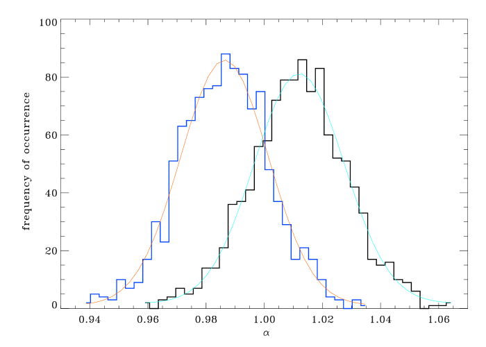
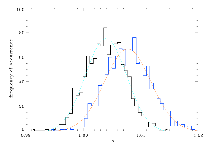
We have performed 1000 realizations for $\alpha=0.7$, $1$ and $1.3$, respectively. Our results for LPE and WE are shown as histograms in Figs. 1 to 6 and summarized in Table 1 where mean values and standard deviations (across realizations) are reported.

Figure 1: LP estimates for $\alpha=0.7$ on ${\bf n}$ (black curve) and ${\tilde{\bf n}}$ (dark blue curve). The bell shaped curves overplotted are Gaussian fits to the data.

Figure 2: Same as Fig. 1 but for WE. Note the shrinking in the horizontal scale.

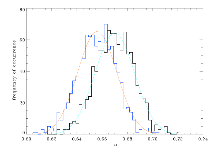
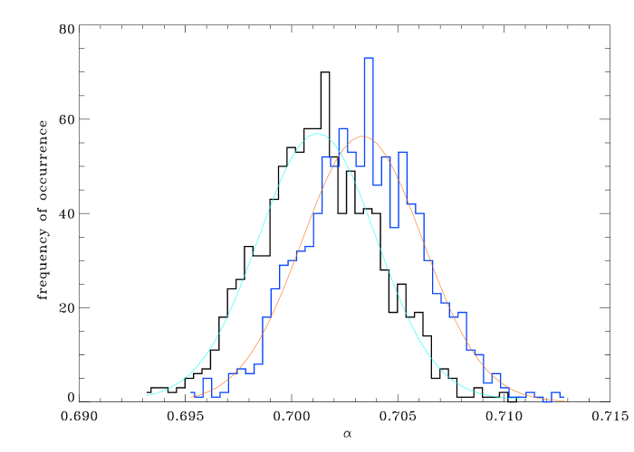
Our first conclusion is that both LPE and WE are not significantly degraded when ${\tilde{\bf n}}$ is considered. In fact, the bias is at most 1% for WE and only slightly larger for LPE. The results for standard deviations are also comparable. Indeed the relative performance of LPE increases as $\alpha$ grows. In general, WE performs slightly better, as expected. However, the simple, robust LPE stands up as a very convincing alternative in the absence of precise a priori information on the functional form of the spectral density. This point will be further discussed below.

We have also implemented the Moulines and Soulier (1999) broad-band log periodogram estimator mentioned in Sect. 2. The resulting estimates, however, were extremely close to those obtained with LPE and we thus decided to omit their presentation for the sake of brevity.

Table 1: Recovery of relevant parameters for WE and LPE

	$0.7$		$1.0$		$1.3$
$\alpha_{\mathrm{input}}$	$\mathbf{n}$	${\tilde{\bf n}}$	$\mathbf{n}$	${\tilde{\bf n}}$	$\mathbf{n}$	${\tilde{\bf n}}$
LPE	$0.671$	$0.657$	$1.013$	$0.988$	$1.361$	$1.314$
${\widehat{\alpha}_{\mathrm{LP}}}$	$\pm 0.015$	$\pm 0.016$	$\pm 0.017$	$\pm 0.016$	$\pm 0.021$	$\pm 0.016$
WE	$0.7015$	$0.7036$	$1.0042$	$1.0082$	$1.3223$	$1.317$
${\widehat{\alpha}_{\mathrm{W}}}$	$\pm 0.0028$	$\pm 0.0029$	$\pm 0.0033$	$\pm 0.0039$	$\pm 0.0054$	$\pm 0.030$

Figure 3: Same as Fig. 1, for $\alpha=1$.

Figure 4: Same as Fig. 2, for $\alpha=1$.

Figure 5: Same as Fig. 1, for $\alpha=1.3$.

Figure 6: Same as Fig. 2, for $\alpha=1.3$.

3.2 Effects on Map Making

In order to understand how WE and LPE impact on map making we evaluated GLS maps out of 50 data streams simulated as discussed in Sect. 3.1. We recall here that the GLS estimate for the map is:

$${\tilde{\bf m}}=({\bf P}^{\prime}{\bf N}^{-1}{\bf P})^{-1}\,{\bf P}^{\prime}{\bf N}^{-1}{\bf d}\,,$$

where $\mathbf{N}$ is the noise covariance matrix introduced in Eq. (7). The Monte Carlo pipeline relies on the following scheme: (1) generation of the noise timestream, $\mathbf{n}$; (2) computation of ${\tilde{\bf n}}$; (3) derivation of WE and LPE. The maps are computed using the iterative map making algorithm discussed in Natoli et al. (2001).

We note that WE return estimates of $A$, $f_{k}$ and $\alpha$. Only the latter two are required to build $\mathbf{N}$, the scale factor being irrelevant. On the other hand, LPE only returns estimates of $\alpha$. So, a fiducial value for $f_{k}$ is used to compute ${\bf N}$. This approach finds its theoretical justification in Dahlhaus (1995). He shows that taking

$$N_{jk}\propto\int_{-\pi}^{\pi}e^{i(j-k)f}f^{-\alpha}df$$ (15)

provides estimates asymptotically equivalent to exact GLS under the only assumption that Eq. (4) holds. Note that Eq. (15) only depends on $\alpha$.

A natural figure of merit to assess the relative performance of LPE and WE is the angular power spectrum of the maps. The latter is computed as

$$C_{\ell}=\frac{1}{2\ell+1}\sum_{m=\ell}^{\ell}|a_{\ell m}|^{2}\,,$$ (16)

where the $a_{\ell m}$’s are coefficients in the spherical harmonic expansion of the noise maps. We are not interested here in a rigorous power spectrum estimation but, rather, in a comparison between LPE and WE. This justifies the use of Eq. (16) which neglects corrections for, e.g., the sky coverage and detailed shape of the surveyed region. The results are shown in Fig. 7 (note that the $C_{\ell}$’s are averaged over the simulation index).

Figure 7: Averaged angular power spectrum of 50 maps displayed as a function of multipole $\ell$. The light blue line is for WE and completely hides the curve for LPE. The bottom red line is the difference between the two. The spectral index input value is $\alpha=1.2$.

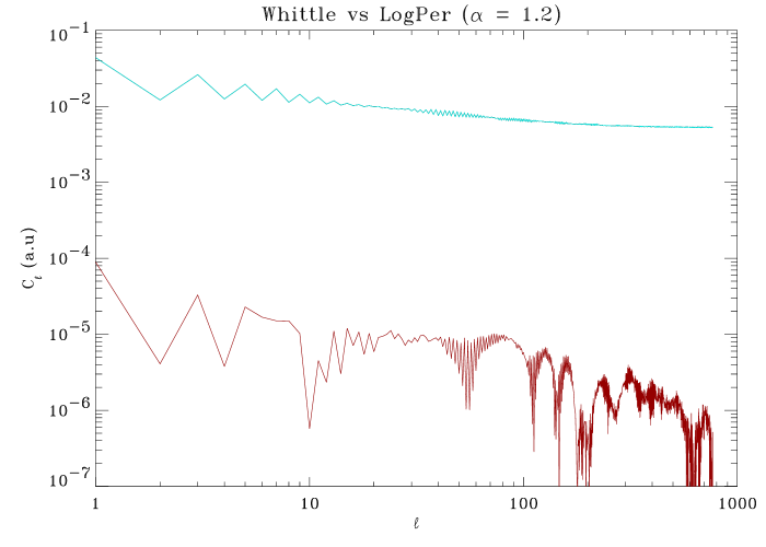
The curves for WE and LPE are virtually indistinguishable. This confirms that only the knowledge of $\alpha$ is relevant for GLS map making. Also, the small differences between LPE and WE become de facto immaterial when map making is at stake. This is an important point: as discussed in Sect. 2, LPE is semiparametric and as such less prone to suffer from a misspecified model.

The heuristic motivation behind this result can be easily understood if we think of GLS map making as equivalent to OLS performed on a pre-filtered series. Pre-filtering needs not to be based on the exact form of the noise spectral density. What really matters is to strongly suppress the long range correlation and this can be achieved even with an imperfect estimate of the noise memory parameter.

3.3 Comparison with iterative methods

The purpose of this Section is to compare the efficiency of LPE and WE against iterative noise-signal estimators. It is generally claimed (Prunet et al. 2001, Doré et al. 2001) that, when reasonable criteria are chosen, convergence on the noise estimator is reached fairly quickly, and only a few ($\sim$ 4 to 5) iterations are sufficient for most applications.

The following scheme is employed to implement the iterative method. We start from the OLS noise estimator, ${\tilde{\bf n}}$. The iteration is carried out by: (1) using the latter to estimate $\mathbf{N}$; (2) performing map making to obtain a new solution for the map, ${\hat{\bf m}}$; (3) estimating the noise again as ${\hat{\bf n}}\equiv{\bf d}-\bf P{\hat{\bf m}}$. This procedure, basically the same described in Prunet et al. (2001) and more recently in Doré et al. (2001), has been implemented by using our map making tool (Natoli et al. 2001), performing 6 iterations (1 OLS plus 5 GLS map making runs) for each map, out of a total of 50 Monte Carlo realizations. In the same spirit of Fig. 7 we derive $C_{\ell}$’s for these maps and compare them with the results based on WE (this time for an input value $\alpha=0.7$). Results are shown in Fig. 8:

Figure 8: As for Fig. 7 but comparing WE (blue curve) with the iterative (light red) method. The input value for $\alpha$ is $0.7$

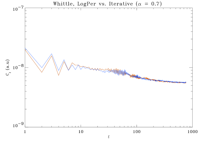
the similarity between the two curves is striking.

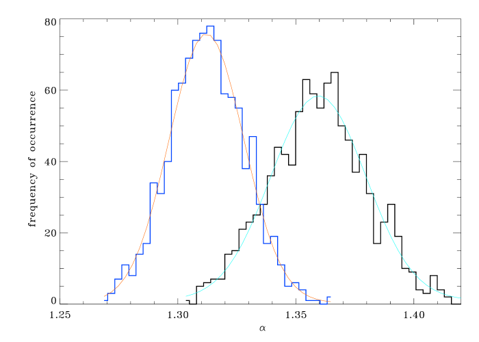
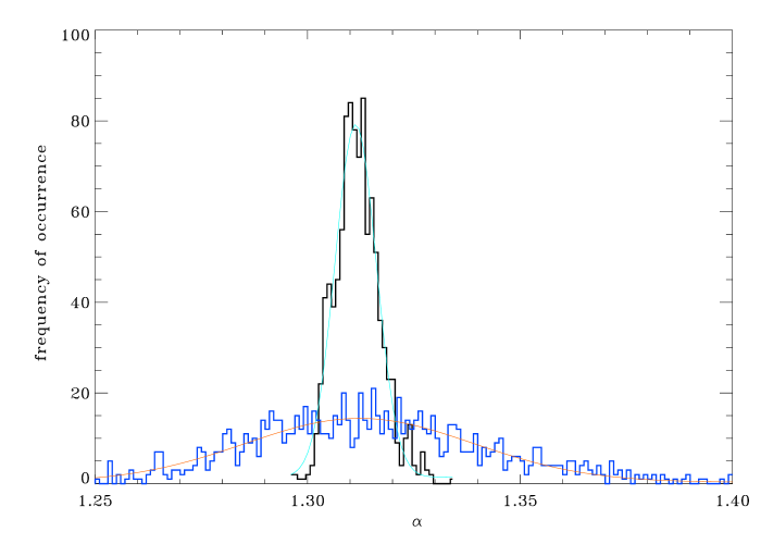
To further compare iterative and non iterative methods we have computed histograms showing the frequency of occurrence of temperature values for selected pixels of the maps. We have chosen a “medium” observed pixel, which is hit 660 times in the Planck scan described above and a “low” observed pixel, hit 240 times. The histograms are shown in Figs. 9 and 10, respectively. Note that all the pixels with the given hit number contribute to the histograms which do not show outliers.

Figure 9: Empirical distribution of the “medium” hit pixels (660 hits). WE (triangles) and the iterative scheme (squares).

Figure 10: Same as Fig. 9 but for pixels observed 240 times.

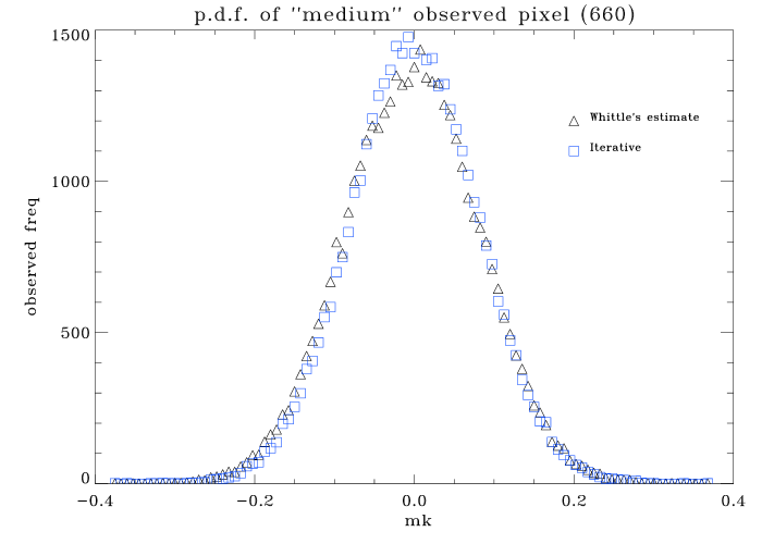
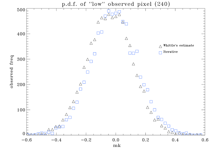
It should be clear at this point that estimating iteratively the noise properties yields no obvious advantage when compared to the simpler WE and LPE described in this paper. Furthermore, as stressed in Sect. 1, the iterative scheme described above needs a sound statistical foundation in the presence of long range dependence. Moreover, it is important to realize that such a scheme is severely more costly than LPE and WE. In fact, in order to implement the latter, only a one step OLS map making is needed, plus one periodogram estimation over the time line and the final GLS one shot map making (the actual computational effort to derive WE and LPE from the periodogram is extremely small). On the other hand, the iterative method requires, other than the OLS map making, a periodogram estimation and a GLS map making at every noise iteration.

3.4 Application to BOOMERanG

All simulations shown above were performed for a subset of the Planck timestream. Furthermore, the noise model assumed as input is the customary “$1/f$” noise (see Eq. (6)). In this Section we relax both assumptions and apply our techniques to BOOMERanG.

BOOMERanG is a balloon borne experiment which scans at constant elevation by allowing the gondola to slew at 1 or 2 degrees per second (d.p.s.), while the detector sampling rate is 60 Hz (de Bernardis et al. 1999). To make our simulations realistic we take a chunk ($2^{22}$ samples out of total of about $3\cdot 10^{7}$) of the 1 d.p.s. part of the scan performed by the B150A channel during the flight of 1998. Contrariously to Planck, this scan is aimed at a small patch. The central region comprises a few tens of square degrees and its coverage (i.e. number of hits per pixel) is far more uniform. The noise properties of the BOOMERanG detectors are not well described by the model given in Eq. (6) because the timestream is altered to deconvolve bolometric filters (both low pass and high pass). To take these effects into account we propose to use:

$$P(f)=A\sin^{2}\left(\frac{\pi f}{2f_{0}}\right)\left[1+\left(\frac{f_{k}}{f}\right)^{\alpha}+A^{\prime}e^{f/f_{1}}\right]$$ (17)

with fiducial values $A\simeq 2\cdot 10^{4}\,(\leavevmode\nobreak\ \mu{\rm K}\sqrt{{\rm s}})^{2}$, $f_{0}\simeq 10^{-3}$ Hz, $f_{1}\simeq 7$ Hz, $f_{k}=0.15$ Hz, $A^{\prime}\sim 10^{8}$ and $\alpha=1.5$. We choose $f_{0}\ll f_{1}$, since the exponential term arises after deconvonvolving the detector high frequency response. To avoid excessive contamination from this high frequency term we sharply cut the spectrum at 20 Hz (as in BOOMERanG: see Hivon et al. 2001).

Figure 11: Same as Figs. 9 and 10, but for a BOOMERanG-like simulation. The histogram are “observed” distributions of GLS mapmaking temperatures for all pixel hit $23$ times in the maps. Noise has been estimated using WE (black curve) and LPE (dark blue).

Figure 12: Same as Fig. 11 but for a pixel hit 100 times. We compare here WE (dark blue curve) with the iterative method (black). The light blue curve is computed using the correct noise power spectrum (Eq. (17)) and, hence, provides the exact GLS estimate.

We thus use Eq. (5) to generate Gaussian noise assuming the power spectrum given in Eq. (17). Subsequently, WE and LPE are applied to the data. WE is fully parametric and requires that a model for the spectral density is specified. Rather than supply the model given by Eq. (17), used to generate the data and hence “exact”, we base the estimations on Eq. (6), i.e. on standard “$1/f^{\prime\prime}$ noise. This results in a deliberate model misspecification, as we are providing WE with an incorrect model. This choice has the obvious purpose to test the robustness of the estimate. Strictly speaking, for $\alpha\leq 2$ Eq. (17) does no longer display long memory behavior, and in this sense we are misleading LPE as well. However, long memory is still a good approximation if $f_{0}\ll f_{k}$.

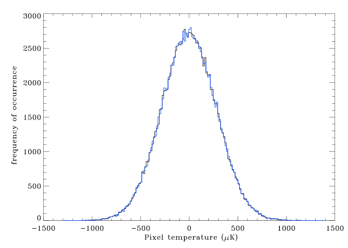
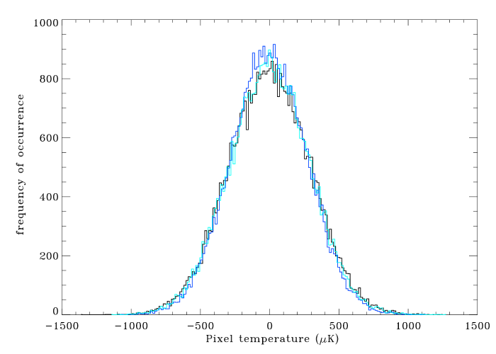
Our results are shown in Fig. 11 where we give, for the most frequently observed pixel in our scan, temperature histograms analogous to the ones given in Figs. 9 and 10. The similarity between the two curves is striking. Very much the same conclusions as in the previous Section can be drawn: the difference between WE and LPE, and between WE and the iterative method, is by all means negligible as shown in Fig. 12. In the same Figure we plot the exact (unfeasible) GLS estimate. Again, no significant difference emerges.

4 Summary and conclusions

This paper has addressed estimation methods for the properties of CMB receiver noise which is well approximated by a long memory process. The most recent literature proves that optimal statistical inference is deeply affected by such characteristics. Under these circumstances results by Dahlhaus (1995) entail that map making procedures can be performed with a single iteration, provided that the slope at the origin of the log spectral density (i.e. $\alpha$) is known; such procedures are asymptotically equivalent to maximum likelihood, GLS-type estimates. Our prime effort, hence, has been to address the efficient estimation of the memory parameter $\alpha$. We have first presented the fully parametric WE which allows for the full correlation structure of the noise process to be recovered. WE, however, requires that the functional form of the noise spectral density is known. To relax this very restrictive assumption we also focus on the semiparametric case, where it is only assumed that a spectral singularity be present at the origin. Both the parametric and the semiparametric procedures are known to enjoy some nice robustness properties in non-standard situations, including non-Gaussian and non-stationary circumstances.

We assess the performance of these statistical procedures by implementing them on simulated Planck and BOOMERanG datasets. We note first that for practical implementation we need to filter out the signal component by running a preliminary OLS regression. We have shown by direct Monte Carlo comparison that this induces no significant degradation of the expected results. Our next conclusion is that the performance of semiparametric LPE is very close to correctly specified, fully parametric WE. This is comforting, as it allows for robust statistical inference under minimal assumptions. In particular, in terms of map making the improvement obtained by a full specification of the noise structure is by all means negligible. Furthermore, our simple map making procedure based on Dahlhaus (1995) ideas provides results which are virtually indistinguishable from those produced by the (computationally much more costly) iterative scheme of Prunet et al. (2001). These results are robust to implementation in the stationary and nonstationary regions.

We believe this paper leaves several avenues for further research. For example, distribution (goodness of fit) tests are profoundly affected by long memory behaviour (Dehling & Taqqu, 1989; Giraitis & Surgailis, 1999). Efficient estimation of $\alpha$ can therefore be exploited to investigate in some detail non-Gaussian features. Also, a correct evaluation of the dependence structure of receiver noise may in principle improve the determination of confidence intervals for the angular power spectrum and its governing parameters, either by resampling methods or by asymptotic approximations. These issues are currently being investigated.