Analytic Approach to the Cloud-in-cloud Problem for Non-Gaussian Density Fluctuations

Abstract

We revisit the cloud-in-cloud problem for non-Gaussian density fluctuations. We show that the extended Press-Schechter (EPS) formalism for non-Gaussian fluctuations has a flaw in describing mass functions regardless of type of filtering. As an example, we consider non-Gaussian models in which density fluctuations at a point obeys a $\chi^{2}$ distribution with $\nu$ degrees of freedom. We find that mass functions predicted by using an integral formula proposed by Jedamzik, and Yano, Nagashima & Gouda, properly taking into account correlation between objects at different scales, deviate from those predicted by using the EPS formalism, especially for strongly non-Gaussian fluctuations. Our results for the mass function at large mass scales are consistent with those by Avelino & Viana obtained from numerical simulations.

NAOJ-Th-Ap2001, No.57

1 Introduction

How many objects with mass $M$ are there in our universe? This question has been one of main interests in the field of cosmological structure formation. Formation process of cosmological objects such as galaxy clusters and galaxies is well understood qualitatively in the context of the hierarchical clustering scenario based on a cold dark matter (CDM) model. In order to compute the number density of collapsed objects or mass function, one must deal with gravitational non-linear growth of small density perturbations. The most direct way is to perform $N$-body simulations. However, performing simulations for a large number of models on wide range of scales is a very difficult task because of the limit of the computation time and available amount of memory. Therefore, it is of great importance to derive analytic formulae that accurately describe the result of $N$-body simulations. Among them, the Press-Schechter formula (Press & Schechter 1974; hereafter PS) has been a most successful one and applied to a wide class of structure formation models.

Nevertheless, the PS formalism has a flaw in describing the number of collapsed objects. Because the underdense region of smoothed density fluctuations is not taken into account in the formalism, integration of the mass function over whole range of mass does not yield a unity. Even if the density fluctuation smoothed on mass scale $M$ is less than a critical density fluctuation $\delta_{c}$, there is a chance that the density fluctuation smoothed on larger mass scale $M^{\prime}>M$ is larger than $\delta_{c}$. This is called the “cloud-in-cloud” problem. Press & Schechter (1974) simply multiplied the mass function by the “PS fudge factor of two”in the case of Gaussian random fields.

The cloud-in-cloud problem for Gaussian random fields have been partially solved by Peacock & Heavens (1990) and Bond et al (1991) using the so-called excursion set formalism and by Jedamzik (1995) and Yano, Nagashima & Gouda (1996) using an integral equation. Consider a density fluctuation $\delta_{M}$ smoothed on mass scale $M$ at a given point. Then one can regard a sequence of density fluctuations $\delta_{M_{1}},\delta_{M_{2}},\cdots$ in descending order of $M$ as a trajectory of a “particle.” For fluctuations smoothed by the sharp $k$-space filter, each trajectory is described by a Markovian random walk of $\delta$ as a function of “time” $M$. Then we analytically obtain the PS fudge factor of two. However, for fluctuations smoothed by other filters, no analytic result is known, since the correlation between fluctuations with different scale renders the motion of a particle non-Markov process.

In contrast, the cloud-in-cloud problem for non-Gaussian density fluctuations had not been explored until recently. As is well known, a number of theoretical “unstandard” models including cosmic string models, texture models, multiple fields models, and so on predict that the primordial fluctuations are not Gaussian. Because the number of collapsed dark matter halos at early epoch, e.g. clusters at $z\sim 1$ or galaxies at $z\gtrsim 5$, depends sensitively on the tails of distribution function of initial density fluctuations, even a small deviation from Gaussianity would cause a noticeable change in the statistical property of those high-redshift objects. To make predictions on the number count of these rare objects, it is of crucial importance to investigate how the PS formalism is extended to models with non-Gaussian initial conditions.

Recently, there has been some progress on this issue based on the so-called extended Press-Schechter (EPS) formalism in which the PS fudge factor is again assumed to be a constant. For Gaussian fluctuations smoothed by the sharp $k$-space filter, the assumption is correct because of the nature of the Markovian random walk of $\delta$. However, in other cases, it is not known whether such assumption is correct, especially for non-Gaussian models. In the context of formalism developed by Jedamzik (1995) and Yano, Nagashima & Gouda (1996), the PS fudge factor is equivalent to the inverse of conditional probability of finding a region where $\delta_{M_{1}}\geq\delta_{c}$ of mass scale $M_{1}$ provided that it is totally included inside an isolated region where $\delta_{M_{2}}=\delta_{c}$ of mass scale $M_{2}$. In other words, the PS fudge factor is not a constant and depends on smoothing scales $M_{1},M_{2}$ in general. This behavior was also noticed by Nagashima & Gouda (1997) using Monte Carlo simulations. Although it has been claimed that the EPS formalism provides a good fit to the mass function obtained from $N$-body simulations for some non-Gaussian models (Robinson & Baker 2000), one cannot immediately give a justification for the result. In fact, recent numerical simulations of linear density fields showed that the EPS formalism does not provide a good fit to the mass function for strongly non-Gaussian probability distribution functions (PDFs) with small variance $\sigma\lesssim 0.5$ which correspond to objects with large mass, such as galaxy clusters at present (Avelino & Viana 2000). For such small variances, the mass function is essentially determined by the abundance of rare density peaks which are sensitive to the non-Gaussianity of initial fluctuations. It is of crucial importance to understand the role of the conditional probability for strongly non-Gaussian density fluctuations, especially at large scales.

In this paper, we study non-Gaussian models in which one-point PDF of density fluctuations smoothed on mass scale $M$ obeys a $\chi^{2}$ distribution with $\nu$ degrees of freedom, which are very simple and widely used as toy models in the literature (e.g. Barreiro, Sanz, Martínez-González & Silk 1998). The degree of non-Gaussianity is characterized by $\nu$. A $\chi^{2}_{\nu}$ distribution is strongly non-Gaussian for small $\nu$ and converges to a Gaussian distribution in the limit $\nu\rightarrow\infty$.

In §2, we introduce a formalism for computing the mass function. In §3, we describe simple models for which a density fluctuation at a point obeys a $\chi^{2}_{\nu}$ distribution. In §4, we explore the property of the conditional probability and compare the obtained mass functions with those predicted by using the EPS formalism. In §5, the effect of mode correlation is discussed. In the last section, we summarize our result and draw our conclusions.

2 Theory of Mass Function

To compute mass functions analytically, PS made following assumptions: (1) the overdense region collapses to an virialized object with mass $M$ when the linear density fluctuation $\delta$ smoothed on mass scale $M$ reaches a critical value $\delta_{c}$ which is a function of cosmic time; (2) Each overdense region is independent and described by a spherically symmetric collapse model which specifies $\delta_{c}$ (Tomita 1969; Gunn & Gott 1972). Then the volume fraction of the collapsing region at initial time with mass scale equal to or larger than $M$ is simply given by

$$\psi(\geq\delta_{c};M)=\int_{\delta_{c}}^{\infty}p(\delta;\sigma(M))d\delta,$$ (1)

where $p(\delta;\sigma(M))$ denotes a one-point PDF with variance $\sigma^{2}(M)\equiv\langle\delta_{M}^{2}\rangle$ of the initial density perturbation. Now consider regions where the density fluctuation $\delta$ smoothed on mass scale $M_{1}$ exceed $\delta_{c}$. Each region should be totally contained inside an isolated collapsed object with mass $M_{2}\geq M_{1}$. Then we have

$$\psi(\geq\delta_{c};M_{1})=\int_{M_{1}}^{\infty}\frac{M_{2}}{\bar{\rho}}n(M_{2})P(M_{1}|M_{2})dM_{2},$$ (2)

where $\bar{\rho}$ denotes the mean cosmic density, $P(M_{1}|M_{2})$ is the conditional probability of finding a region $V_{1}$ of mass scale $M_{1}$ where $\delta_{1}\equiv\delta(M_{1})\geq\delta_{c}$ provided that $V_{1}$ is totally contained in an isolated overdense region $V_{2}$ where $\delta_{2}\equiv\delta(M_{2})=\delta_{c}$ (Jedamzik 1995). In this formulation, one can calculate the mass function by solving the integral equation (2), once the conditional probability $P(M_{1}|M_{2})$ and the one-point PDF of the smoothed density fluctuations are given. Note that the excursion set formalism developed by Bond et al. (1991) is essentially equivalent to this formalism. Because $V_{2}$ is an isolated region, the conditional probability is given by the probability of the first upcrossing of $\delta_{2}$ at the threshold $\delta_{c}$ when smoothed on decreasing mass scales

$$P(M_{1}|M_{2})=p(\delta_{1}\geq\delta_{c}|\delta_{2}=\delta_{c},\delta(M)<\delta_{c},^{\forall}M>M_{2}),$$ (3)

assuming that the spatial correlation in the density fluctuations is negligible. Let us call a sequence of density fluctuations $\delta(M_{1}),\delta(M_{2}),\cdots$ in descending order of $M$ as a trajectory of a particle. For fluctuations $\delta(M)$ smoothed by the sharp $k$-space filter whose phases of Fourier modes $\delta_{\mathbf{k}}$ are uncorrelated, the motion of a particle is described by a Markovian random walk. In this case, the conditional probability $P(M_{1}|M_{2})$ does not depend on the state of a particle before the crossing $\delta_{2}=\delta_{c}$,

$$P(M_{1}|M_{2})=p(\delta_{1}\geq\delta_{c}|\delta_{2}=\delta_{c}).$$ (4)

In what follows we assume that equation (4) gives a good approximation of the conditional probability for fluctuations smoothed by other filters (Yano, Nagashima & Gouda 1996). Then we only need to specify a one-point PDF and a two-point PDF of the smoothed density fluctuations at a given point.

If $P(M_{1}|M_{2})\equiv f$ does not depend on mass scales $M_{1}$ and $M_{2}$, then the mass function is described by a formula similar to the PS formula, where the PS fudge-factor, $f$, is related to the conditional probability as

$$f=[p(\delta_{1}\geq\delta_{c}|\delta_{2}=\delta_{c})]^{-1}=const.$$ (5)

Let us first consider the Gaussian models. The bivariate Gaussian two-point PDF with vanishing means is given by

$$p_{G}(\delta_{1},\delta_{2};\sigma_{1},\sigma_{2},\tau)d\delta_{1}d\delta_{2}=$$ (6)

$$\frac{1}{2\pi\sigma_{1}\sigma_{2}\sqrt{1-\tau^{2}}}\exp\Biggl{[}-\frac{(\frac{\delta_{1}}{\sigma_{1}})^{2}+(\frac{\delta_{2}}{\sigma_{2}})^{2}-2\tau(\frac{\delta_{1}}{\sigma_{1}}\frac{\delta_{2}}{\sigma_{2}})}{2(1-\tau^{2})}\Biggr{]}d\delta_{1}d\delta_{2},$$

where $\sigma_{i}^{2}$ denotes the variance of $\delta_{i}$, $\langle\delta_{i}^{2}\rangle$, and $\tau$ denotes the correlation coefficient, $\langle\delta_{1}\delta_{2}\rangle/\sigma_{1}\sigma_{2}$. Note that $p_{G}$ is scale-invariant, i.e. $p_{G}(x_{1},x_{2};\sigma_{1},\sigma_{2},\tau)=\sigma_{1}^{-1}\sigma_{2}^{-1}p_{G}(x_{1}/\sigma_{1},x_{2}/\sigma_{2},;1,1,\tau)$. For fluctuations smoothed by the sharp $k$-space filter, $\tau=\sigma_{2}/\sigma_{1}$ (see appendix). Then the two-point conditional PDF is written in terms of the one-point PDF as $p_{G}(\delta_{1}|\delta_{2})=p_{G}(\delta_{1},\delta_{2})/p_{G}(\delta_{2})=p_{G}(\delta_{1}-\delta_{2};\sqrt{\sigma_{1}^{2}-\sigma_{2}^{2}})$. Because the Gaussian one-point PDF is also scale-invariant, we recover the constant PS fudge factor, $f_{G}^{-1}=p_{G}(\delta_{1}\geq\delta_{c}|\delta_{2}=\delta_{c})=({2\pi})^{-1/2}\int_{0}^{\infty}\exp[-\delta^{2}/2]d\delta=1/2$. From equations (2) and (4), we obtain an explicit form of mass function,

$$n(M;\delta_{c})dM=-\frac{f\bar{\rho}}{M}\frac{\partial\psi(\geq\delta_{c};M)}{\partial M}dM.$$ (7)

In general, however, the PS fudge factor $f$ is not a constant and the mass function $n(M)$ cannot be written explicitly as in equation (7). For instance, for Gaussian fluctuations smoothed by other window functions, $P(M_{1}|M_{2})$ depends on smoothing scales $M_{1}$ and $M_{2}$ (Nagashima 2001).

In the non-Gaussian models, the mass scale dependence of $P(M_{1}|M_{2})$ must be always taken into account. However, Koyama, Soda & Taruya (1999; hereafter KST) claimed that for generic non-Gaussian models, the relation $p(\delta_{1}|\delta_{2})\simeq p(\delta_{1}-\delta_{2})$ holds for $M_{1}\ll M_{2}$. Consequently, we have

$$P(M_{1}|M_{2})\approx\int_{0}^{\infty}p(\delta_{1},\sigma_{1})d\delta_{1}.$$ (8)

If the one-point PDF is scale-invariant, the above integration yields a constant value. Although obtaining a similar relation for all scales $M_{1}\leq M_{2}$ is a more complex issue, KST and some authors evaluated mass functions by solving equation (7) assuming a constant $f$ for various non-Gaussian models (Koyama, Soda & Taruya 1999; Robinson & Baker 2000). From now on, we call the PS formalism using the approximation described by equations (7) and (8) in evaluating the mass function, the extended PS (EPS) formalism.

Now let us evaluate the validity of the EPS formalism. In the limit of vanishing correlation coefficient, $\tau\rightarrow 0$, or equivalently $M_{1}\ll M_{2}$, the two-point PDF is written as a direct product of one-point PDFs, $p(\delta_{1},\delta_{2})=p(\delta_{1})p(\delta_{2})$, which gives

$$P(M_{1}|M_{2})=\int_{\delta_{c}}^{\infty}p(\delta_{1};\sigma_{1})d\delta_{1}.$$ (9)

On small mass scales with large variance, i.e. $\sigma_{1}\gg\delta_{c}$, the lower limit of integration variable $\delta_{c}$ can be set to zero as in the Gaussian fluctuations smoothed by the sharp $k$-space filter, leading to a constant $f$. Hence, the EPS approximation is valid for scales $M_{1}\ll M_{2}$ and $\sigma_{1}\gg\delta_{c}$. However, on large mass scales, where $\sigma_{1}\lesssim\delta_{c}$, such approximation cannot be verified except for the Gaussian cases, since the contribution of integration of $p(\delta_{1};\sigma_{1})$ in $\delta_{1}$ from $0$ to $\delta_{c}$ cannot be negligible. Therefore, the EPS approximation is not valid for $\sigma_{1}\lesssim\delta_{c}$ though $M_{1}\ll M_{2}$. This contradicts the validity of the EPS approximation for $M_{1}\ll M_{2}$ that KST have claimed. In generic non-Gaussian PDFs, the relation $p(\delta_{1}|\delta_{2})\sim p(\delta_{1}-\delta_{2})$ for $M_{1}\ll M_{2}$ does not hold. In fact, the class of PDFs of density fluctuations that satisfy $p(\delta_{1}|\delta_{2})\sim p(\delta_{1}-\delta_{2})$ for $M_{1}\ll M_{2}$ is very limited. The Gaussian fluctuations smoothed by the sharp $k$-space filter belong to this very limited class.

It would be worthwhile to comment on relationship between the conditional probability and the excursion set formalism. If the conditional probability satisfies $p(\delta_{1}|\delta_{2})=p(\delta_{1}-\delta_{2})$, then the master equation can be reduced to the diffusion equation by using the Kramers-Moyal expansion which is used in the excursion set formalism. However, it is clear that general PDFs do not necessarily satisfy the diffusion equation. We need to derive a proper two-point PDF that corresponds to the density fluctuation distribution function under consideration.

3 $\chi^{2}$ models

We consider toy models in which the density fluctuation $\delta_{M}$ smoothed on scale $M$ at a given point obey a $\chi^{2}_{\nu}$ PDF and we assume that the Fourier modes of fluctuations $\delta_{\mathbf{k}}$ are totally uncorrelated. The validity of this assumption is discussed in §5.

Let ${\mathbf{x}}_{i}=(x_{1i},x_{2i},\cdots,x_{Ni}),i=1,\cdots,\nu$ be independent Gaussian $N$-dimensional vector variables. We call the distribution of ${\mathbf{z}}\equiv(\sum_{i=1}^{\nu}x_{1i}^{2},\sum_{i=1}^{\nu}x_{2i}^{2},\cdots,\sum_{i=1}^{\nu}x_{Ni}^{2})$ a $N$-point $\chi^{2}$ distribution with $\nu$ degrees of freedom. The one-point $\chi^{2}_{\nu}$ distribution is

$$p_{\chi^{2}_{\nu}}(x;\sigma)dx=\frac{\sqrt{\nu/2}}{\sigma\Gamma(\nu/2)}\left(\sqrt{\frac{\nu}{2}}\frac{x}{\sigma}\right)^{(\nu-2)/2}\exp\left(-\sqrt{\frac{\nu}{2}}\frac{x}{\sigma}\right)dx,$$ (10)

where $\Gamma(x)$ denotes the $\Gamma$ function.

Next, we derive the two-point PDF $p(z_{1},z_{2})$ of $\chi^{2}_{\nu}$ distribution with variance $\sigma_{1}$, $\sigma_{2}$ and correlation coefficient $\tau$. Let us consider variables $x_{1},x_{2}$ which obey a two-point Gaussian distribution $p_{G}(x_{1},x_{2};s_{1},s_{2},\epsilon)$ with vanishing means. By changing the variables as $z_{1}=x_{1}^{2}$, $z_{2}=x_{2}^{2}$, one obtains

$$p_{\chi_{1}^{2}}(z_{1},z_{2};\tau)dz_{1}dz_{2} = \frac{1}{2\pi s_{1}s_{2}\sqrt{(z_{1}z_{2})(1-\epsilon^{2})}}\cosh\Biggl{[}\frac{\epsilon\sqrt{z_{1}z_{2}}}{s_{1}s_{2}(1-\epsilon^{2})}\Biggr{]}$$ (11)

$$\times\exp\Biggl{[}-\frac{s_{2}z_{1}/s_{1}+s_{1}z_{2}/s_{2}}{2s_{1}s_{2}(1-\epsilon^{2})}\Biggr{]}dz_{1}dz_{2},$$

where $s_{i}^{2}\equiv\langle x_{i}^{2}\rangle=\langle z_{i}\rangle$, $\sigma_{i}^{2}=2s_{i}^{4}$ and $\tau=(\langle z_{1}z_{2}\rangle-\langle z_{1}\rangle\langle z_{2}\rangle)/\sigma_{1}\sigma_{2}=\epsilon^{2}$. The corresponding characteristic function is

$$\phi_{\chi^{2}_{1}}(t_{1},t_{2})=[1-2is_{1}s_{2}(s_{1}t_{1}s_{2}^{-1}+s_{2}t_{2}s_{1}^{-1})-4s_{1}^{2}s_{2}^{2}(1-\epsilon^{2})t_{1}t_{2}]^{-1/2}.$$ (12)

The characteristic function for $p_{\chi^{2}_{\nu}}(z_{1},z_{2};\sigma_{1},\sigma_{2},\tau)$ is given by $\phi_{\chi^{2}_{\nu}}=(\phi_{\chi^{2}_{1}})^{\nu}$ where $\langle z_{i}\rangle=\nu s_{i}^{2}$, Var$(z_{i})=\sigma^{2}_{i}=2\nu s_{i}^{4}$ and $\tau=\epsilon^{2}$, since each variable $z_{i}$ is written as a sum of independent random variables. From two-dimensional Fourier transform of $\phi_{\chi^{2}_{\nu}}(t_{1},t_{2})$, we finally obtain the two-point PDF of $\chi^{2}_{\nu}$ distribution,

$$p_{\chi^{2}_{\nu}}(z_{1},z_{2};\sigma_{1},\sigma_{2},\tau)$$ (18)

$$=\left\{\begin{array}[]{l}\displaystyle\frac{1}{\alpha\tilde{\sigma}^{2}\Gamma(\frac{\nu}{2})}\Biggl{(}\frac{z_{1}z_{2}}{\tau\tilde{\sigma}^{2}}\Biggr{)}^{\frac{\nu}{4}-\frac{1}{2}}\exp\Biggl{[}-\frac{\sigma_{1}^{-1}z_{1}+\sigma_{2}^{-1}z_{2}}{\alpha\sqrt{2/\nu}}\Biggr{]}\\ \displaystyle\quad\times\textrm{I}_{\frac{\nu}{2}-1}\Biggl{(}\frac{\sqrt{4\tau z_{1}z_{2}}}{\alpha\tilde{\sigma}}\Biggr{)},\hfil\textrm{for}\quad 0<\tau<1,\\ \displaystyle\frac{1}{\alpha\tilde{\sigma}^{2}\Gamma(\frac{\nu}{2})}\Biggl{(}\frac{-z_{1}z_{2}}{\tau\tilde{\sigma}^{2}}\Biggr{)}^{\frac{\nu}{4}-\frac{1}{2}}\exp\Biggl{[}-\frac{\sigma_{1}^{-1}z_{1}+\sigma_{2}^{-1}z_{2}}{\alpha\sqrt{2/\nu}}\Biggr{]}\par\\ \displaystyle\quad\times\textrm{J}_{\frac{\nu}{2}-1}\Biggl{(}\frac{\sqrt{-4\tau z_{1}z_{2}}}{\alpha\tilde{\sigma}}\Biggr{)},\hfil\textrm{for}\quad-1<\tau<0,\\ \displaystyle\frac{1}{\tilde{\sigma}^{2}(\Gamma(\frac{\nu}{2}))^{2}}\Biggl{(}\frac{z_{1}z_{2}}{\tilde{\sigma}^{2}}\Biggr{)}^{\frac{\nu}{2}-1}\exp\Biggl{[}-\frac{\sigma_{1}^{-1}z_{1}+\sigma_{2}^{-1}z_{2}}{\sqrt{2/\nu}}\Biggr{]},\quad\textrm{for}\quad\tau=0,\end{array}\right.$$

where $\alpha\equiv 1-\tau$, $\tilde{\sigma}\equiv\sqrt{2\sigma_{1}\sigma_{2}/\nu}$ and $J_{n}$ and $I_{n}$ are the Bessel and modified Bessel function of the first kind, respectively. The one-point and the two-point $\chi^{2}_{\nu}$ PDFs are scale-invariant and extend from $0$ to $\infty$ for each variable. Because we assume that the PDFs of a density fluctuation have a vanishing mean, we will use off-centered PDFs, $p^{*}_{\chi^{2}_{\nu}}(z)\!\equiv\!p_{\chi^{2}_{\nu}}(z+\langle z\rangle)$, $p^{*}_{\chi^{2}_{\nu}}(z_{1},z_{2})\!\equiv\!p_{\chi^{2}_{\nu}}(z_{1}+\langle z_{1}\rangle,z_{2}+\langle z_{2}\rangle)$ which are also scale-invariant in the following analysis.

It is cumbersome to calculate the three-point PDF explicitly. For simplicity, we only consider the case of $\nu=1$ (see also Sheth 1995). In terms of the covariance matrix for the original trivariate Gaussian PDF,

$$\textrm{cov}=\left(\begin{array}[]{@{\,}ccc@{\,}}s_{11}&s_{12}&s_{13}\\ s_{21}&s_{22}&s_{23}\\ s_{31}&s_{32}&s_{33}\end{array}\right),$$ (19)

the explicit form of the trivariate $\chi^{2}_{1}$ PDF can be written as

$$p_{\chi_{1}^{2}}(z_{1},z_{2},z_{3};\sigma_{1},\sigma_{2},\sigma_{3},\sigma_{12},\sigma_{23},\sigma_{13})$$ (20)

$$= \frac{1}{2(2\pi)^{3/2}\sqrt{\textrm{det}(\textrm{cov})z_{1}z_{2}z_{3}}}\exp\Bigl{[}-\frac{c_{11}z_{1}+c_{22}z_{2}+c_{33}z_{3}}{2}\Bigr{]}$$

$$\times \Bigl{(}\exp(-c_{12}\sqrt{z_{1}z_{2}})\cosh(c_{23}\sqrt{z_{2}z_{3}}+c_{13}\sqrt{z_{1}z_{3}})$$

$$+ \exp(c_{12}\sqrt{z_{1}z_{2}})\cosh(-c_{23}\sqrt{z_{2}z_{3}}+c_{13}\sqrt{z_{1}z_{3}})\Bigr{)},$$

where $\sigma_{ij}=2s_{ij}^{2}$ for $i\neq j$, $\sigma_{i}^{2}=2s_{ii}^{2}$, and $c_{ij}=(\textrm{cov}^{-1})_{ij}$.

It should be noted that the models considered in our analysis are not exactly identical to the “$\chi^{2}_{\nu}$ field models” (Peebles 1999; Scoccimarro 2000) in which the initial fluctuation itself is described by a $\chi^{2}_{\nu}$ field. In contrast to the Gaussian models, the PDF of a smoothed $\chi^{2}$ field deviates from the original PDF in general (Avelino & Viana 2000). If one would like to explore more realistic models, one should take into account the dependence of the PDF on smoothing scale. Fortunately, for $\chi^{2}_{\nu}$ PDFs with $\nu$ larger than $10$ smoothed by the Gaussian filter, it is known that the departure from the original PDF is not significant although the departure is noticeable in the case of the sharp $k$-space filter (Avelino & Viana 2000). Hence, we can expect a similar result for some particular choice of smoothing filter.

4 Solving the cloud-in-cloud problem

In order to study the characteristics of $\chi^{2}_{\nu}$ models on mass function, we first estimate the conditional probability

$$P(M_{1}|M_{2})\equiv\int_{\delta_{c}}^{\infty}p^{*}_{\chi^{2}_{\nu}}(\delta_{1}|\delta_{c};\sigma_{1},\sigma_{2},\tau)d\delta_{1}$$ (21)

for various kinds of smoothing filters, such as the sharp $k$-space, the Gaussian and the top-hat filters.

First of all, we consider fluctuations smoothed by the sharp $k$-space filter $\tilde{W}_{R}(k)=6R^{3}\theta(\pi/R-k)/\pi$. The relation between the mass $M$ and the smoothing scale $R$ is given by $M=6R^{3}\bar{\rho}/\pi$. The correlation coefficient is $\tau=\sigma_{2}/\sigma_{1}=(M_{1}/M_{2})^{(n+3)/6}$ (see appendix) provided that the power spectrum of the initial density fluctuations has a form ${\cal{P}}(k)\propto k^{n}$, where $n$ denotes the spectral index and $n>-3$. The critical value $\delta_{c}$ is 1.69 independent of mass scale for the spherical collapse in the Einstein-de Sitter universe. For simplicity, we assume $\delta_{c}=1.69$ in the following analysis. As we have argued in §2, for $M_{1}\ll M_{2}$ and $\sigma_{1}\gg\delta_{c}$, the EPS approximation gives a correct value,

$$f^{-1}(\textrm{EPS}) = \int_{0}^{\infty}p^{*}_{\chi^{2}_{\nu}}(\delta_{1};\sigma_{1})d\delta_{1}$$ (22)

$$= \frac{\Gamma(\nu/2,\nu/2)}{\Gamma(\nu/2)}$$

$$= P(M_{1}|M_{2})\quad\mbox{for}~{}M_{2}\gg M_{1}~{}\mbox{and}~{}\sigma_{1}\gg\delta_{c},$$

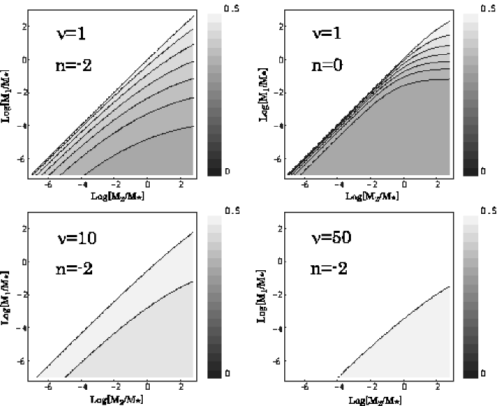
Figure 1: Plots of the conditional probability $p(\delta_{1}\geq\delta_{c}|\delta_{2}=\delta_{c};\sigma(M_{1}),\sigma(M_{2}),\tau(M_{1},M_{2}))$ for $\chi^{2}_{\nu}$ PDFs smoothed by the sharp $k$-space filter. $n$ denotes the spectral index. The accompanying palettes show the relation between the gray level and the value. $M_{*}$ is defined as $\sigma(M_{*})=1$. We set $\delta_{c}=1.69$.

where $\Gamma(x,y)$ denotes the incomplete Gamma function. For other parameter regions, however, the EPS approximation is not always correct, especially for strongly non-Gaussian PDFs. From Figure 1, one can see that the inverse of the EPS factor, $f^{-1}$, deviates from the correct conditional probability $P(M_{1}|M_{2})$ for a region $M_{1}\ll M_{2}$ and $\sigma_{1}\lesssim\delta_{c}$, or equivalently $M_{1}\gtrsim M_{*}$, where $\sigma(M_{*})=1$. For fluctuations smoothed by the sharp $k$-space filter, the trajectories are described by a Markovian random walk. Therefore, the chance of upcrossing at the critical value $\delta_{c}$ is almost equivalent to the chance of downcrossing at $\delta_{c}$, i.e. $P(M_{1}|M_{2})=1/2$. Therefore, in the neighborhood of diagonal line $M_{1}=M_{2}$, we have $P(M_{1}|M_{2})\sim 1/2$. On the other hand, in the Gaussian limit $\nu\rightarrow\infty$, we have $f^{-1}(\textrm{EPS})=\Gamma(\nu/2,\nu/2)/\Gamma(\nu/2)\rightarrow 1/2$. Consequently, for weakly non-Gaussian PDFs smoothed by the sharp $k$-space filter such that $f^{-1}(\textrm{EPS})\sim 1/2$, it is natural to expect $P(M_{1}|M_{2})\sim 1/2$ on all scales $M_{1}\leq M_{2}$. Thus, for weakly non-Gaussian PDFs smoothed by the sharp $k$-space filter, the EPS formalism gives a good approximation of $f$.

Next, we consider the property of fluctuations smoothed by other filters for which the trajectories of density fluctuations cannot be described by a Markovian random walk because of the Fourier-mode correlation. In this case, equation (4) does not give an exact result. Let us consider a trajectory that firstly crosses $\delta_{c}$ upwards at $M_{2}$ and ends at $\delta_{1}>\delta_{c}$ and $M_{1}$. For $M_{2}\gg M_{1}$, the trajectory can be well approximated by that of a Markovian random walk, since the correlation length is almost negligible compared with the length of the whole trajectory. On the other hand, for $M_{2}\sim M_{1}$, the trajectory can be well approximated by a monotonically increasing function in decreasing value of $M$, or increasing value of $\sigma$, since the correlation coefficient is almost equal to unity. Then the conditional probability is approximately given by

$$P(M_{1}|M_{2})\approx\int_{\delta_{c}}^{\infty}p(\delta_{1}|\delta_{2}=\delta_{c},\partial\delta_{2}/\partial M_{2}<0)d\delta_{1}.$$ (23)

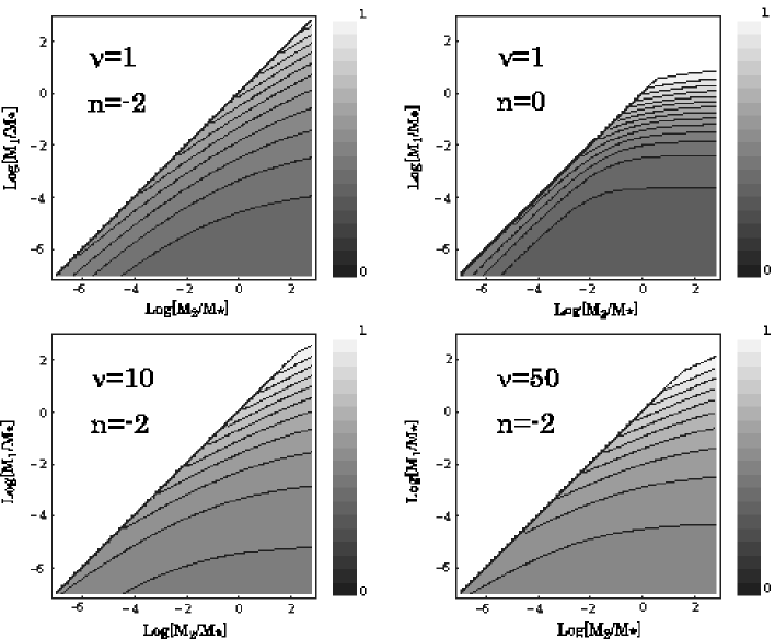
Figure 2: Same as Figure 1, but for the Gaussian filter. Note that the contour level is from 0 to 1.

At large scales, $\delta_{1}\ll\delta_{c}$, or equivalently $M_{1}\gg M_{*}$, the probability of upcrossing at $\delta_{c}$ is very low. In other words, the probability of $\partial\delta_{2}/\partial M_{2}\geq 0$ at $\delta_{2}=\delta_{c}$ is almost zero. Therefore, the extra condition $\partial\delta_{2}/\partial M_{2}>0$ is not necessary at large scales. As shown in Figure 2, when the Gaussian filter is used, $P(M_{1}|M_{2})$ increases compared with that for the sharp $k$-space filter owing to the Fourier-mode correlation. At large scales $M_{1}\gg M_{*}$, $P(M_{1}|M_{2})\sim 1$. Consequently, the chance of downcrossing at $\delta_{c}$ is almost zero. Thus it is reasonable to conclude that equation (4) still provides a good approximation of mass functions, at least, at large scales even for other filters. On the other hand, in the region $M_{1}\ll M_{*}$ and $M_{1}\ll M_{2}$, $P(M_{1}|M_{2})$ is close to the value in the case of the sharp $k$-space filter. This suggests that the approximation of the Markovian random walk is good in that parameter region.

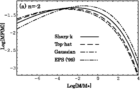
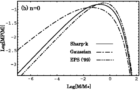
Figure 3: Plots of multiplicity functions $F(M)=Mn(M)/\bar{\rho}$ for fluctuations obeying the $\chi^{2}_{1}$ PDF smoothed by various filters. (a)$n=-2$. (b)$n=0$. The solid, the dashed, and the dashed-dotted lines correspond to $F(M)$ for fluctuations smoothed by the sharp $k$-space filter, the top-hat filter, and the Gaussian filter, respectively. The dashed-double-dotted line represents the value predicted by using the EPS formalism. $M_{*}$ is defined as $\sigma(M_{*})=1$. In the case of $n=0$, the multiplicity function $F(M)$ for fluctuations smoothed by the top-hat filer is exactly the same as that smoothed by the sharp $k$-space filter.

Substituting the variances $\sigma_{1}$, $\sigma_{2}$, and the correlation coefficient $\tau$ for each type of smoothing filter (see appendix for derivation) into the conditional probability equation (4), one can compute the mass function by solving the integral equation (2). In Figure 3, we show the multiplicity functions $F(M)$ for the various filters and for the EPS formalism in the case of $\chi^{2}_{1}$ PDF with one degree of freedom. The multiplicity functions derived here decrease at large scales compared with those of the EPS prediction. As we have argued in §2, the actual value of $P(M_{1}|M_{2})=p(\delta_{1}\geq\delta_{c}|\delta_{2}=\delta_{c})$ is larger than the value $f^{-1}$ predicted by using the EPS approximation at large scales, which explains a decrease in the multiplicity function $F(M)$. To compensate the deficit at large scales, $F(M)$ increases at small scales. Regarding the dependence of $F(M)$ on the spectral index $n$, one can see in Figure 3 that a relative increase of $F(M)$ at small scales is much prominent for larger $n$. This is because $F(M)$ decreases rapidly at smaller scales for a larger value of $n$, or for a much blue spectrum. Similar behavior is also observed for the Gaussian models (Nagashima 2001).

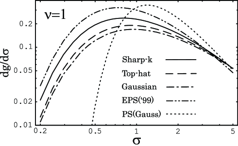
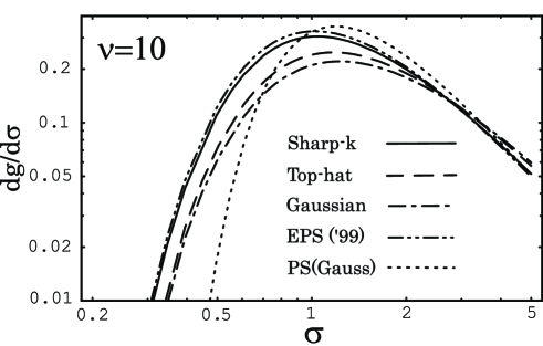
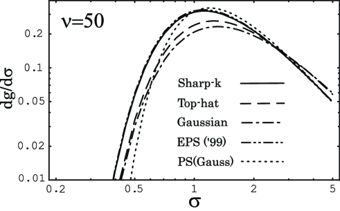
Figure 4: Plots of $dg/d\sigma$ for fluctuations that obey three kinds of $\chi^{2}$ PDFs ($\nu=1,10$ and 50). The spectral index is assumed to be $n=-2$. The solid, the dashed, and the dashed-dotted lines correspond to $F(M)$ for fluctuations smoothed by the sharp $k$-space filter, the top-hat filter and the Gaussian filter, respectively. The dashed-double-dotted line represents the value predicted by the EPS formalism. The dotted line corresponds to the value predicted by the PS formalism for the Gaussian PDF. In the case of the sharp-k space filter, $dg/d\sigma$ does not depend on $n$.

In Figure 4, we show, for $\chi^{2}_{\nu}$ PDFs with various degree of freedom, $dg(\sigma)/d\sigma$ which is defined as $g(\sigma)=\tilde{g}(M(\sigma))$ for which $\tilde{g}(M)=\int_{M}^{\infty}F(M^{\prime})dM^{\prime}$ is the fraction of collapsed objects above a smoothing scale $M$. At large scales, $\sigma\lesssim 1$, $dg(\sigma)/d\sigma$ is significantly increased compared with those corresponding to the Gaussian PS mass function. This is because the $\chi^{2}_{\nu}$ PDFs have a broad tail toward large $\delta$, especially for strongly non-Gaussian PDFs with small value of $\nu$. Even in the case of $\nu=50$, one can still observe a clear difference from the value corresponding to the PS mass function for fluctuations with small variance $\sigma\lesssim 1$. In other words, the amount of rare density peaks at large scales is very sensitive to the non-Gaussianity of the initial fluctuations. In the Gaussian limit, $\nu\rightarrow\infty$, the EPS formalism correctly reproduces $dg(\sigma)/d\sigma$ for fluctuations smoothed by the sharp $k$-space filter. As the degree of freedom $\nu$ decreases, a deviation from the EPS prediction becomes noticeable. It is clear that the EPS formalism overestimates the number density of dark halos on large scales $\sigma\lesssim 1$, especially for strongly non-Gaussian PDFs. For fluctuations smoothed by the Gaussian and the top-hat filters, such a deviation is prominent even in the case of a weakly non-Gaussian PDF ($\nu=50$) owing to the correlation between Fourier-modes. Similar result has been obtained by Avelino & Viana (2000) using Monte Carlo simulations for smoothed $\chi^{2}_{\nu}$ fields.

Note that our analytic calculation of $dg(\sigma)/d\sigma$ for $\nu=10$ and $\sigma\lesssim 1$ agrees well with the previous numerical results by Avelino & Viana (2000) when the Gaussian filter is used. The result is natural, since the departure from the original one-point PDF is not significant in this case. However, for fluctuations smoothed by the Gaussian filter with slightly large variance $1\!\lesssim\!\sigma\!\lesssim\!5$, our analytic values exceed their numerical values. We might be able to recover their numerical results if we use the improved approximation described by equation (23) of the conditional probability instead. Nevertheless, for the purpose of constraining non-Gaussianity of initial fluctuations using the abundance of high-redshift clusters (Matarrese, Verde & Jimenez 2000), our approximation of the conditional probability may be sufficient in practice, as mentioned.

5 Effect of mode correlation

So far, we have assumed that different Fourier-modes of $\chi^{2}_{\nu}$ fluctuations are uncorrelated. However, if we consider $\chi^{2}_{\nu}$ field models defined as $\phi(\textbf{x})\equiv\sum_{i}^{\nu}\psi_{i}^{2}(\textbf{x})$ where $\psi_{i}(\textbf{x})$ are independent homogeneous and isotropic random Gaussian fields whose Fourier-modes are uncorrelated, Fourier-modes $\phi_{\textbf{k}}$ of a $\chi^{2}_{\nu}$ field are no longer uncorrelated. The signature of correlation appears as non-vanishing skewness , kurtosis, or higher-order cumulants although the two-point correlation has the same form as the Gaussian one (Scoccimarro 2000). In this case, a hypothetical particle with position $\delta(M)$ cannot be described by the Markovian random walk even if we smooth the fluctuations by using the sharp-k space filter. Therefore, it is of crucial importance to estimate the effect of correlation.

In order to check the validity of our calculation, we compare the conditional probability $P_{3}\equiv p(\delta_{1}\geq\delta_{c}|\delta_{2}=\delta_{c},\delta_{3}<\delta_{2}),M_{1}\leq M_{2}\leq M_{3}$ specified by a three-point and two-point PDFs to $P_{2}\equiv p(\delta_{1}\geq\delta_{c}|\delta_{2}=\delta_{c})$ specified by a two-point and one-point PDFs. In fact, the actual condition to be satisfied is equation (3), which is equivalent to $P_{n},n\rightarrow\infty$. $P_{3}$ is expected to be more accurate than $P_{2}$ for estimating the conditional probability $P(M_{1}|M_{2})$.

In what follows, we only consider $\nu=1$ case, for which the effect of mode correlation owing to the non-Gaussianity is most significant. In the limit $\sigma_{3}\rightarrow 0$, the correlation coefficients vanish $\tau_{i3}\sim\sigma_{3}/\sigma_{i}\rightarrow 0$, which gives $p(\delta_{1}|\delta_{2},\delta_{3})=p(\delta_{1},\delta_{2})p(\delta_{3})/p(\delta_{2})p(\delta_{3})=p(\delta_{1}|\delta_{2})$. Thus, if $M_{3}$ is large enough compared with $M_{2}$ and $M_{1}$, the effect of mode correlation is negligible. On the other hand, for $M_{3}\sim M_{2}$, or equivalently, $\sigma_{3}\sim\sigma_{2}$, the probability of having a trajectory $\delta_{1}\geq\delta_{c}$ becomes large owing to the correlation in the fluctuations on different scales. Note that in the limit $\sigma_{3}\rightarrow\sigma_{2}$, $P_{3}$ is equivalent to the right-hand-side of equation (23) assuming that $\delta_{2}(\sigma_{2})$ is differentiable at $\sigma_{2}$. From equation (20), one can easily calculate the ratio $P_{3}/P_{2}$.

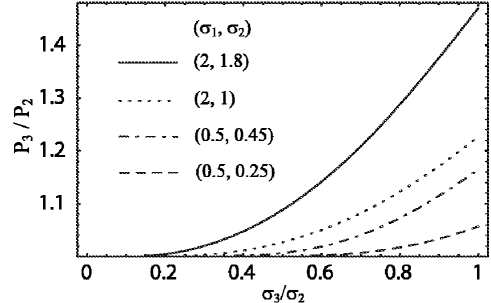
Figure 5: Effect of mode correlation in the case of Gaussian filtering for $\chi^{2}_{1}$ fluctuations with the spectral index $n=-2$. A deviation from 1 in the value of $P_{3}/P_{2}$ gives a relative error in $P_{2}$ for estimating the conditional probability $P(M_{1}|M_{2})$ assuming that the effects of four-point or higher-order correlations are negligible.

First of all, we consider the case of the Gaussian filtering. It turns out that the ratio $P_{3}/P_{2}$ is $\lesssim 1.5$ for $\sigma_{1}=2$, and $\lesssim 1.2$ for $\sigma_{1}=0.5$ if the spectral index is $n=-2$ (see figure 5). At large scales $\sigma<1$, a decrease in the multiplicity function $F(M)$ is expected to be less than $\sim 30$ percent.

In the case of the sharp-k space filtering, we have the scale-invariant relations in the covariances: $\sigma_{12}=\sigma_{2}^{2},\sigma_{23}=\sigma_{3}^{2},\sigma_{13}=\sigma_{3}^{2}$. Then we obtain

$$p_{\chi_{1}^{2}}^{SK}(z_{1}|z_{2},z_{3})$$

$$= p_{\chi_{1}^{2}}^{SK}(z_{1}|z_{2})$$

$$= \frac{1}{\sqrt{2\pi z_{1}(s_{1}^{2}-s_{2}^{2})}}\exp\Biggl{(}-\frac{z_{1}+z_{2}}{2(s_{1}^{2}-s_{2}^{2})}\Biggr{)}\cosh\Biggl{(}\frac{\sqrt{z_{1}z_{2}}}{s_{1}^{2}-s_{2}^{2}}\Biggr{)},$$ (25)

where $\sigma_{i}^{2}=2s_{i}^{4}$, which gives $P_{3}=P_{2}$ irrespective of the value of the spectral index $n$ as in the case of the Gaussian fluctuations. Thus, the effect of three-point correlation is completely negligible if the fluctuations are smoothed by using the sharp-k space filter. This relation might also hold for other $\chi^{2}_{\nu}$ PDFs with $\nu>1$, since the effect of correlation is less significant. Presumably, all the scale-invariant PDFs have this property.

To summarize, the effect of mode correlation is less significant for fluctuations at large scales $\sigma<1$ irrespective of the type of filtering. Inclusion of an additional condition $\delta_{3}<\delta_{c}$ improves the reliance of calculation for strongly non-Gaussian fluctuations at small scales $\sigma>1$.

6 Conclusions

In this paper, we have demonstrated that the EPS approach has a drawback in describing the number of collapsed objects, especially for strongly non-Gaussian density fluctuations. Based on the formalism developed by Jedamzik, and Yano, Nagashima and Gouda properly taking into account the scale dependence of correlation between objects at different scales, we analytically calculated the mass function for various $\chi^{2}_{\nu}$ models and found a deviation from those predicted by using the EPS formalism, especially noticeable for strongly non-Gaussian models: a decrease at large scales and an increase at small scales in the value of multiplicity function. The result may affect some recent studies of constraints on non-Gaussian models using the cluster abundance at different red shifts and the correlation length of galaxy clusters (Chin, Ostriker & Strauss 1998; Koyama, Soda & Taruya 1999; Robinson, Gawiser & Silk 2000). Our results are similar to those by Avelino and Viana (2000) based on Monte-Carlo simulations of non-Gaussian $\chi^{2}_{\nu}$ fields. At intermediate scales, $1\lesssim\sigma\lesssim 5$, the deviation from the EPS prediction is not prominent. It seems that the result is consistent with those from $N$-body simulations for various non-Gaussian fields (Robinson & Baker 2000). It would be interesting if larger $N$-body simulation could be carried out and find out a deviation of mass function from the EPS prediction for objects with very large mass (low-$\sigma$) or for those with very small mass (high-$\sigma$).

In order to vindicate that the generalized PS formalism works in estimating the mass function for non-Gaussian models, we should take various kinds of effects into consideration: effects of non-spherical collapse (for Gaussian fields, see Sheth et al 2001), ambiguity in mass-smoothing scale relation (Bardeen et al 1986, Peacock & Heavens 1991), and conditions of objects surrounding by an isolated dark halo. The last issue is relevant to the cloud-in-cloud problem. Although we have discussed about a prescription for incorporating the condition of upcrossing at the critical value $\delta_{c}$, we did not explicitly consider the effect of spatial correlation owing to the finite size of halos in evaluating the conditional probability $P(M_{1}|M_{2})$. For Gaussian models it is known that the effect of spatial correlation almost cancels out the filtering effect, recovering the original PS mass function, particularly in the case of the top-hat filter (Nagashima 2001). It is of very importance to check whether such a cancellation occurs for non-Gaussian models. The other issues left untouched should be addressed in our future work.

Appendix A Correlation coefficients

In this section, we derive the formulae of correlation coefficients $\tau$ for density fluctuations smoothed by three types of filter, namely, the sharp $k$-space filter, the Gaussian filter and the top-hat filter.

Let us consider a mass density fluctuation (contrast) $\delta({{\mathbf{x}}})\equiv\frac{\rho({{\mathbf{x}}})-\bar{\rho}}{\bar{\rho}}$, where $\rho({{\mathbf{x}}})$ denotes the mass density at a point ${{\mathbf{x}}}$ and $\bar{\rho}$ is the mean cosmic mass density. Using a window function $W_{R}(r=|x|)$, $\delta({{\mathbf{x}}})$ can be smoothed on scale $R$

$$\delta_{R}({\mathbf{x}})=\int W_{R}(|{\mathbf{x}}-{\mathbf{x}}^{\prime}|)\delta({\mathbf{x}}^{\prime})d{\bf x},$$ (A1)

and in Fourier space,

$$~{}~{}=\frac{1}{(2\pi)^{3}}\int\tilde{W}_{R}(k)\delta({\mathbf{k}})e^{i{\bf k\cdot x}}d{{\mathbf{k}}},$$ (A2)

where $\delta_{\mathbf{k}}$ and $\tilde{W}_{R}(k)$ are the Fourier transforms of $\delta_{\mathbf{k}}$ and $W_{R}(r)$, respectively. Here we choose a normalization of the window function as $W_{R}(0)=1$.
If the fluctuations are homogeneous, then the two-point correlation is written in terms of the power spectrum ${\cal{P}}(k)$ as

$$\langle\delta_{{\mathbf{k}}_{1}}\delta^{*}_{{\mathbf{k}}_{2}}\rangle=(2\pi)^{3}\delta_{D}({\mathbf{k}}_{1}-{\mathbf{k}}_{2}){\cal{P}}(k_{1}).$$ (A3)

which gives

$$\langle(\delta_{R})^{2}\rangle=\frac{1}{(2\pi)^{3}}\int_{0}^{\infty}4\pi k^{2}\tilde{W}_{R}^{2}(k){\cal{P}}(k)dk.$$ (A4)

The correlation coefficient is given by $\tau\equiv\langle\delta_{R_{1}}\delta_{R_{2}}\rangle/\sigma_{R_{1}}\sigma_{R_{2}}$ where

$$\langle\delta_{R_{1}}\delta_{R_{2}}\rangle=\frac{1}{(2\pi)^{3}}\int_{0}^{\infty}4\pi k^{2}\tilde{W}_{R_{1}}(k)\tilde{W}_{R_{2}}(k){\cal{P}}(k)dk.$$ (A5)

Note that all the equations in this appendix except for (A3) hold for fluctuations whose Fourier transforms are correlated. The mass of objects smoothed on scale $R$ can be defined as

$$M\equiv\int{\bar{\rho}}W_{R}({\mathbf{x}})d{\mathbf{x}}.$$ (A6)

The correlation coefficients for the three types of filters are written as follows. We assume that ${\cal{P}}(k)\propto k^{n}$.

1. Sharp $k$-space filter
   

   $$W_{R}(r) = \frac{3}{k_{c}^{3}r^{3}}(\sin k_{c}r-k_{c}r\cos k_{c}r),$$ (A7)

   $$\tilde{W}_{R}(k) = \frac{6\pi^{2}}{k_{c}^{3}}\theta(k_{c}-k),$$ (A8)

   where $k_{c}$ is the cut-off wave number, $k_{c}\simeq R^{-1}$, and $\theta(x)$ is the Heaviside step function. Note that there is an ambiguity in the relation between $k_{c}$ and $R$. Here we define it as $k_{c}=\pi/R$ that gives $M=6R^{3}\bar{\rho}/\pi$ which has been widely used in the literature. If we choose $k_{c}=(9\pi/2)^{1/3}/R$, then we have $M=4\pi R^{3}\bar{\rho}/3$. For the former definition, the variance of density fluctuation is

   $$\sigma_{M}^{2}\propto\frac{R^{-3-n}\pi^{1+n}}{2(3+n)},$$ (A9)

   and the correlation coefficient for $M_{1}<M_{2}$ is $\tau=\sigma_{M_{2}}/\sigma_{M_{1}}=(M_{2}/M_{1})^{-(n+3)/6}=(R_{2}/R_{1})^{-(n+3)/2}$.

2. Gaussian filter
   

   $$W_{R}(r) = \exp(-r^{2}/(2R^{2})),$$ (A10)

   $$\tilde{W}_{R}(k) = (2\pi)^{3/2}R^{3}\exp(-k^{2}R^{2}/2).$$ (A11)

   The mass of objects smoothed on scale $R$ is $M=(2\pi)^{3/2}R^{3}\bar{\rho}$ and for $n>-3$,

   $$\sigma_{M}^{2} \propto (2\pi)^{-2}R^{-3-n}\Gamma((3+n)/2),$$ (A12)

   $$\tau = \frac{2^{(n+3)/2}(\sigma_{1}^{-4/(3+n)}+\sigma_{2}^{-4/(3+n)})^{-(3+n)/2}}{\sigma_{1}\sigma_{2}}.$$ (A13)

3. Top-hat filter
   

   $$W_{R}(r) = \theta(1-r/R),$$ (A14)

   $$\tilde{W}_{R}(k) = 4\pi R^{3}\Biggl{(}\frac{\sin kR}{(kR)^{3}}-\frac{\cos kR}{(kR)^{2}}\Biggr{)}.$$ (A15)

   The mass of objects smoothed on scale $R$ is $M=4\pi R^{3}\bar{\rho}/3$. If $n$ is not an integer, for $-3<n<1$,

   $$\sigma_{M}^{2}\propto\frac{9}{2\pi^{2}R^{3}}(2R)^{-n}(n-2)(n+1)\sin(n\pi/2)\Gamma(-3+n),$$ (A16)

   $$\tau = \frac{9\sin(n\pi/2)}{4\pi^{2}R_{1}^{3}R_{2}^{3}}\Biggl{(}\biggl{(}(R_{1}+R_{2})^{3-n}-(R_{2}-R_{1})^{3-n}\biggr{)}(\Gamma(-3+n)+\Gamma(-2+n))$$ (A17)

   $$+ \biggl{(}(R_{1}+R_{2})^{1-n}-(R_{2}-R_{1})^{1-n}\biggr{)}R_{1}R_{2}\Gamma(-1+n)\Biggr{)}\sigma_{1}^{-1}\sigma_{2}^{-2}.$$

   For integers $-3<n<1$,

   $$\sigma_{M}^{2}\propto\frac{9}{2\pi^{2}R^{3}}(2R)^{-n}\times\left\{\begin{array}[]{ll}\displaystyle{\frac{\pi}{6}}~{}~{}~{}(n=0)&\\ \\ \displaystyle{\frac{1}{8}~{}~{}~{}(n=-1)}&\\ \\ \displaystyle{\frac{\pi}{60}~{}~{}~{}(n=-2)}&,\end{array}\right.\\$$ (A18)

   and

   $$\tau=\left\{\begin{array}[]{ll}\displaystyle{\sqrt{\frac{R_{1}^{3}}{R_{2}^{3}}}=\frac{\sigma_{2}}{\sigma_{1}},~{}~{}(n=0)}&\\ \\ \displaystyle{\frac{1}{4R_{1}^{2}R_{2}^{2}}\biggl{(}2R_{1}R_{2}(R_{1}^{2}+R_{2}^{2})+(R_{2}^{2}-R_{1}^{2})^{2}\ln\frac{R_{1}-R_{2}}{R_{1}+R_{2}}\biggr{)},~{}~{}~{}(n=-1)}&\\ \\ \displaystyle{\frac{5R_{2}^{2}-R_{1}^{2}}{4R_{2}^{3}}\sqrt{R_{1}R_{2}}=\frac{\sigma_{2}}{4\sigma_{1}^{5}}(5\sigma_{1}^{4}-\sigma_{2}^{4}),~{}~{}~{}(n=-2)}.&\end{array}\right.\\$$ (A19)

References

- (1)
- (2) Avelino, P.P., & Viana, P.T.P. 2000, MNRAS, 314, 358
- (3) Barreiro, R.B., Sanz, J.L., Martínez-González, E., & Silk, J. 1998, MNRAS, 296, 693
- (4) Bond, J.R., Cole, S., Efstathiou, G., & Kaiser, N. 1991, ApJ, 379, 440
- (5) Bardeen, J.M., Bond, J.R., Kaiser, N., & Szalay A.S., 1986, ApJ, 304, 15
- (6) Chiu, W.A., Ostriker, J.P., & Strauss, M.A. 1998, ApJ, 479, 490
- (7) Gunn,J.E., & Gott, J.R. 1972, ApJ, 176, 1
- (8) Jedamzik, K. 1995, ApJ, 448, 1
- (9) Koyama, K., Soda, J., & Taruya, A. 1999, MNRAS, 310, 111
- (10) Matarrese, S., Verde, L., & Jimenez, R. 2000, ApJ, 541, 10
- (11) Nagashima, M., 2001, ApJ, 562, 7
- (12) Nagashima, M., & Gouda, N. 1997, MNRAS, 287, 515
- (13) Peebles, P.J.E. 1999, ApJ, 510, 523
- (14) Peacock, J.A., & Heavens, A.F. 1990, MNRAS, 243, 133
- (15) Press, W.H., & Schechter, P. 1974, ApJ, 187, 425
- (16) Robinson, J., & Baker, J.E. 2000, MNRAS, 311, 781
- (17) Robinson, J., Gawiser E., Silk, J. 2000, ApJ, 532, 1
- (18) Sheth, R.K., 1995, MNRAS, 277, 933
- (19) Sheth, R.K., Mo, H.J., & Tormen, G. 2001 MNRAS, 323, 1
- (20) Scoccimarro, R. 2000, ApJ, 542, 1
- (21) Tomita, K. 1969, PTP, 42,9
- (22) Yano, T., Nagashima, M, & Gouda, N. 1996, ApJ, 466, 1