Rotational velocities of A-type stars ^,

Within the scope of a Key Programme determining fundamental parameters of stars observed by HIPPARCOS, spectra of 525 B8 to F2-type stars brighter than $V=8$ have been collected at ESO. Fourier transforms of several line profiles in the range 4200–4500 Å are used to derive $v\sin i$ from the frequency of the first zero. Statistical analysis of the sample indicates that measurement error is a function of $v\sin i$ and this relative error of the rotational velocity is found to be about 6 % on average.
The results obtained are compared with data from the literature. There is a systematic shift from standard values from Slettebak et al. (1975), which are 10 to 12 % lower than our findings. Comparisons with other independent $v\sin i$ values tend to prove that those from Slettebak et al. are underestimated. This effect is attributed to the presence of binaries in the standard sample of Slettebak et al., and to the model atmosphere they used.

1 Introduction

Since work began on the subject (Struve & Elvey 1931), it has been observed that stellar rotation rate is directly linked to the spectral type, and A-type stars are known to be mean high rotators.

The Doppler effect allows measurement of the broadening parameter $v\sin i$, the projection of the equatorial velocity $v$ along the line of sight. From a statistically significant sample of measured $v\sin i$, it is possible to derive the distribution of $v$ assuming that the rotation axes are randomly distributed and the sample is not biased.

Projected rotational velocities can be derived in many ways. Although large surveys of $v\sin i$ already exist, great care must be taken when combining their data, as various calibrations were used.

The most accurate method of computing $v\sin i$ would be the time-consuming computation of line profiles, starting from a model atmosphere (with the introduction of other broadening mechanisms), and their comparison with the observed lines (see Dravins et al. 1990, for their study of Sirius). Such high precision is not justified, however, in a statistical study of high rotators like the non-peculiar A-type stars where other mechanisms (macroturbulence, instrumental) are negligible compared to rotation.

Line widths appear to be the natural indicator for measuring stellar rotation, and most $v\sin i$ are derived in this way, as a function of the full-width at half-maximum (FWHM). The largest catalogue of $v\sin i$ is by Uesugi & Fukuda (1982). It is an extremely heterogeneous compilation of observational data mainly based on the old Slettebak system (Slettebak 1949, 1954, 1955, 1956; Slettebak & Howard 1955). Several years ago, Abt & Morrell (1995) measured $v\sin i$ for 1700 A-type stars in the northern hemisphere, calibrated with the new system from Slettebak et al. (1975, hereafter SCBWP). More recently, Wolff & Simon (1997) measured the $v\sin i$ of 250 stars, most of which were cooler than those in our sample, by cross-correlation with the spectra of standard stars of similar temperature. They found a small systematic difference with Abt & Morrell’s results (the former are larger by $\approx 5$ %), and with those of Danziger & Faber (1972) (smaller by 8 %). This can be explained by the difference between the “old” and “new” Slettebak systems. Brown & Verschueren (1997) derived $v\sin i$ for a sample of early-type stars in Sco OB2 association from spectra taken with the same instrument we used. They adopted three different techniques according to the expected $v\sin i$ values, which they show to be generally consistent with each other. The $v\sin i$ values so obtained correspond to those defining the SCBWP scale, except for stars with $v\sin i$ below 60 $\mathrm{km}\,\mathrm{s}^{-1}$, for which the SCBWP values are systematically lower.

The use of the Fourier technique in the determination of $v\sin i$ remains occasional, mainly because using a calibration FWHM-$v\sin i$ is much easier and fitting theoretical profiles to observed ones in wavelength space allows one to derive more parameters than simply the rotational broadening. Nevertheless, Fourier techniques are a valuable tool for investigating stellar rotation, as described by Smith & Gray (1976). Gray (1980) compared the $v\sin i$ obtained from Fourier transform of the Mg ii 4481 line profile with the $v\sin i$ values from Uesugi & Fukuda and SCBWP and found a reasonable agreement (deviations of $\pm 10$ % with SCBWP), but his sample is quite small.

Suspecting that the small differences found with respect to standard values could be due to an underestimation in the SCBWP calibration of the $v\sin i$ values, we decided to undertake a measure of $v\sin i$ independent of any pre-existing calibration. We adopted the method described in Ramella et al. (1989).

The largest scatter in the average $v\sin i$ distribution is found for late B and early A stars (Gray 1992, Fig. 17.16 p. 386), and we want to test whether this is due only to errors in measurement or if it is related to some physical effect. Brown & Verschueren (1997), in their study of the Sco OB2 association, found that B7-B9 stars of the Upper Scorpius subgroup rotate faster than the B0-B6 stars. This result corresponds to Gray’s result, suggesting that the apparent scatter may disguise a physical effect. This effect has already been detected by Mouschovias (1983).

The possibility of a change on average $v\sin i$ with evolution from zero-age to terminal-age main sequence has been studied for several decades, and the absence of any evolutionary effect for stars with a mass higher than $1.6\,\mathscr{M}_{\odot}$ is confirmed by the recent study of Wolff & Simon (1997). The fact that the colors of stars are affected by rotation was observed for the first time by Brown & Verschueren, but only for stars belonging to young groups, not field stars. They conclude, moreover, that the determination of ages and mass distributions is not affected by rotation.

As a matter of fact, the effect of rotation on stellar parameters is also known: a rapidly rotating star simulates a star with lower $T_{\mathrm{eff}}$ and $\log g$. However, in this case, all quantities (line strength, photometric colors, for example) change in the same way so that the effect is practically undetectable (this point was already discussed by Wolff 1983, p. 159), especially when field stars are studied.

In this paper, newly determined $v\sin i$ data, obtained with Fourier transforms, for 525 southern early-type stars are presented. The observations and the sample are described in Sect. 2. In Sect. 3 the technique used to derive $v\sin i$ from the spectra is detailed and discussed. In Sect. 4 the results are presented and compared to data from the literature. In Sect. 5 our conclusions are summarized. This paper is the first of a series pertaining to rotational velocities of A-type stars; data collected in the northern hemisphere and measured $v\sin i$ will be presented in a forthcoming paper.

2 Observational data

The spectra were obtained with the ECHELEC spectrograph, mounted at the Coudé focus of the ESO 1.52 m telescope at La Silla. They were collected from June 1989 to January 1995 in the framework of an ESO Key Programme aimed at the determination of fundamental parameters of early-type stars observed by HIPPARCOS (Gerbaldi & Mayor 1989), nearer than 100 pc. In total, 871 spectra were collected for 525 stars whose spectral types range from B8 to F2 (Fig. 1). Most of these stars belong to the main sequence (half of the sample are in luminosity class V, and a fifth is classified IV or IV-V). These stars are all brighter than the $V$ magnitude 8.

It is worth noticing that the spectra which are the subject of the present paper were also studied by Grenier et al. (1999) to derive radial velocities, and that the 71 A0 dwarf stars observed were investigated by Gerbaldi et al. (1999). Basically, this sample includes objects with no radial velocity or only for one epoch. Some stars with no $v\sin i$ determination were added from the Bright Star Catalogue (Hoffleit & Jaschek 1982). The observational programme is more detailed by Grenier et al. (1999).

Figure 1: Distribution of the spectral type for the 525 programme stars.

Figure 2: Normalized spectrum of Sirius, covering the 4210–4500 Å range, around H$\gamma$. The 15 selected lines (listed in Table 2) are indicated

The observations were made in the spectral range 4210–4500 Å (Fig. 2). The linear dispersion is about 3.1 Å $\mathrm{mm}^{-1}$, the slit width of $320\,\mu$m corresponds to $1\aas@@fstack{\prime\prime}52$ on the sky, and the power of resolution is about 28 000.

The complete reduction of the spectra using MIDAS package, from CCD frame to linear spectrum, is detailed by Burnage & Gerbaldi (1990, 1992).

3 Measurement of the rotational velocity

3.1 Method

As pointed out by Gray & Garrison (1987), there is no “standard” technique for measuring projected rotational velocity. The first application of Fourier analysis in the determination of stellar rotational velocities was undertaken by Carroll (1933). Gray (1992) uses the whole profile of Fourier transform of spectral lines to derive the $v\sin i$, instead of only the zeroes as suggested by Carroll. The $v\sin i$ measurement method we adopted is based on the position of the first zero of the Fourier transform (FT) of the line profiles (Carroll 1933). The shape of the first lobe of the FT allows us to better and more easily identify rotation as the main broadening agent of a line compared to the line profile in the wavelength domain. FT of the spectral line is computed using a Fast Fourier Transform algorithm. The $v\sin i$ value is derived from the position of the first zero of the FT of the observed line using a theoretical rotation profile for a line at 4350 Å and $v\sin i$ equal to 1 $\mathrm{km}\,\mathrm{s}^{-1}$ (Ramella et al. 1989). The whole profile in the Fourier domain is then compared with a theoretical rotational profile for the corresponding velocity to check if the first lobes correspond (Fig. 3).

Figure 3: Profile of the Fourier transform of the Mg ii 4481 Å line (solid line) for the star HIP 95965 and theoretical rotational profile (dashed line) with $v\sin i=200$ $\mathrm{km}\,\mathrm{s}^{-1}$.

If $\nu_{\mathrm{o}}$ is the position of the first zero of the line profile (at $\lambda_{\mathrm{o}}$) in the Fourier space, the projected rotational velocity is derived as follows:

$$v\sin i={4350\over\lambda_{\mathrm{o}}}\,{\nu_{\mathrm{T}}\over\nu_{\mathrm{o}}},$$ (1)

where 4350 Å and ${\nu_{\mathrm{T}}}$ respectively stand for the wavelength and the first zero of the theoretical profile.

It should be noted that we did not take into account the gravity darkening, effect that can play a role in rapidly rotating stars when velocity is close to break-up, as this is not relevant for most of our targets.

3.2 Continuum tracing

Determination of the projected rotational velocity requires normalized spectra.

As far as the continuum is concerned, it has been determined visually, passing through noise fluctuations. The MIDAS procedure for continuum determination of 1D-spectra has been used, fitting a spline over the points chosen in the graphs.

Uncertainty related to this determination rises because the continuum observed on the spectrum is a pseudo-continuum. Actually, the true continuum is, in this spectral domain, not really reached for this type of stars. In order to quantify this effect, a grid of synthetic spectra of different effective temperatures (10 000, 9200, 8500 and 7500 K) and different rotational broadenings has been computed from Kurucz’ model atmosphere (Kurucz 1993), and Table 1 lists the differences between the true continuum and the pseudo-continuum represented as the highest points in the spectra.

Table 1: Differences between the true continuum and the highest points in different spectral bands for the set of synthetic spectra.

$T_{\mathrm{eff}}$, $v\sin i$		spectral interval (Å)
(K, $\mathrm{km}\,\mathrm{s}^{-1}$)		4200–4220	4220–4240	4240–4260	4260–4280	H$\gamma$	4400–4420	4420–4440	4440–4460	4460–4480	4480–4500
10 000,	10	0.0029	0.0028	0.0035	0.0053		0.0042	0.0023	0.0016	0.0012	0.0006
10 000,	50	0.0031	0.0044	0.0043	0.0073		0.0057	0.0032	0.0023	0.0020	0.0011
10 000,	100	0.0041	0.0059	0.0067	0.0077		0.0063	0.0034	0.0040	0.0034	0.0022
9200,	10	0.0049	0.0049	0.0064	0.0090		0.0068	0.0038	0.0027	0.0021	0.0012
9200,	50	0.0058	0.0071	0.0077	0.0123		0.0085	0.0057	0.0046	0.0027	0.0023
9200,	100	0.0076	0.0097	0.0110	0.0140		0.0093	0.0063	0.0070	0.0050	0.0054
8500,	10	0.0073	0.0073	0.0100	0.0143		0.0105	0.0059	0.0047	0.0032	0.0020
8500,	50	0.0099	0.0109	0.0133	0.0202		0.0151	0.0105	0.0069	0.0044	0.0047
8500,	100	0.0142	0.0152	0.0190	0.0262		0.0156	0.0127	0.0140	0.0069	0.0114
7500,	10	0.0037	0.0037	0.0051	0.0069		0.0055	0.0027	0.0023	0.0014	0.0009
7500,	50	0.0083	0.0101	0.0166	0.0225		0.0132	0.0118	0.0064	0.0032	0.0068
7500,	100	0.0212	0.0189	0.0257	0.0381		0.0182	0.0191	0.0255	0.0064	0.0245

It illustrates the contribution of the wings of H$\gamma$, as the hydrogen lines reach their maximum strength in the early A-type stars, and in addition, the general strength of the metallic-line spectrum which grows with decreasing temperature. In the best cases, i.e. earliest type and low broadening, differences are about a few 0.1 %. For cooler stars and higher rotators, they reach up to 3 %. The points selected to anchor the pseudo-continuum are selected as much as possible in the borders of the spectra, where the influence of the wings of H$\gamma$ is weaker.

Continuum is then tilted to origin and the spectral windows corresponding to lines of interest are extracted from the spectrum in order to compute their FT.

3.3 Set of lines

3.3.1 a priori selection

The essential step in this analysis is the search for suitable spectral lines to measure the $v\sin i$. The lines which are candidates for use in the determination of rotation (Table 2) have been identified in the Sirius atlas (Furenlid et al. 1992) and retained according to the following criteria:

• not blended in the Sirius spectrum,

• far enough from the hydrogen line H$\gamma$ to maintain relatively good access to the continuum.

These are indicated in Fig. 2.

Table 2: List of the spectral lines used (when possible) for the $v\sin i$ measurement.

wavelength	element	wavelength	element
(Å)		(Å)
4215.519	Sr ii	4404.750	Fe i
4219.360	Fe i	4415.122	Fe i
4226.728	Ca i	4466.551	Fe i
4227.426	Fe i	4468.507	Ti ii
4235.936	Fe i	4481${}^{.126}_{.325}$	Mg ii †
4242.364	Cr ii	4488.331	Ti ii
4261.913	Cr ii	4489.183	Fe ii
		4491.405	Fe ii

† Wavelengths of both components are indicated for the magnesium doublet line.

The lines selected in the Sirius spectrum are valid for early A-type stars. When moving to stars cooler than about A3-type stars, the effects of the increasing incidence of blends and the presence of stronger metallic lines must be taken into account. The effects are: (1) an increasing departure of the true continuum flux (to which the spectrum must be normalized) from the curve that joins the highest points in the observed spectrum, as mentioned in the previous subsection, and (2) an increased incidence of blending that reduces the number of lines suitable for $v\sin i$ measurements. The former effect will be estimated in Sect. 3.4. The latter can be derived from the symmetry of the spectral lines.

Considering a line, continuum tilted to zero, as a distribution, moments of $k$-th order can be defined as:

$$\forall k,\;m_{k}={\displaystyle\sum_{i=1}^{L}\left[1-\mathscr{F}(\lambda_{i})\right]\left[\lambda_{i}-\lambda_{\mathrm{c}}\right]^{k}\over\displaystyle\sum_{i=1}^{L}1-\mathscr{F}(\lambda_{i})},$$ (2)

for an absorption line centered at wavelength $\lambda_{\mathrm{c}}$ and spreading from $\lambda_{1}$ to $\lambda_{L}$, where $\mathscr{F}(\lambda_{i})$ is the normalized flux corresponding to the wavelength $\lambda_{i}$. Ranges $[\lambda_{1},\lambda_{L}]$ are centered around theoretical wavelengths from Table 2 and the width of the window is taken to be 0.35, 0.90 and 1.80 Å for rotational broadening 10, 50 and 100 $\mathrm{km}\,\mathrm{s}^{-1}$ respectively (the width around the Mg ii doublet is larger: 1.40, 2.0 and 2.3 Å). Skewness is then defined as

$$\gamma_{1}={m_{3}\over(m_{2})^{3/2}}.$$ (3)

Variations of skewness of a synthetic line profile with temperature and/or rotational broadening should be caused only by the presence of other spectral lines that distort the original profile. Table 3 gives skewness of the selected lines for the different synthetic spectra.

Table 3: Variation of the skewness $\gamma_{1}$ (Eq. 3) of the lines with $T_{\mathrm{eff}}$ and $v\sin i$ in the synthetic spectra.

	$v\sin i$	$T_{\mathrm{eff}}$ (K)
line	($\mathrm{km}\,\mathrm{s}^{-1}$)	10 000	9200	8500	7500
Sr ii 4216	10	$0.07$	$0.10$	$0.18$	$0.22$
	50	$0.04$	$0.08$	$0.18$	$0.36$
	100	$0.05$	$0.10$	$0.17$	$0.24$
Fe i 4219	10	$0.03$	$0.03$	$0.04$	$0.05$
	50	$0.03$	$0.08$	$0.18$	$0.32$
	100	$-0.03$	$-0.05$	$-0.07$	$-0.03$
Ca i 4227	10	$-0.02$	$-0.07$	$-0.25$	$-0.63$
	50	$-0.21$	$-0.28$	$-0.37$	$-0.49$
	100	$-0.15$	$-0.22$	$-0.32$	$-0.40$
Fe i 4227	10	$-0.09$	$-0.13$	$-0.19$	$-0.28$
	50	$-0.34$	$-0.48$	$-0.57$	$-0.69$
	100	$-0.26$	$-0.36$	$-0.46$	$-0.55$
Fe i 4236	10	$-0.03$	$-0.06$	$-0.11$	$-0.24$
	50	$-0.01$	$-0.03$	$-0.09$	$-0.24$
	100	$-0.29$	$-0.30$	$-0.31$	$-0.29$
Cr ii 4242	10	$0.01$	$-0.01$	$0.04$	$0.42$
	50	$0.03$	$0.04$	$0.10$	$0.25$
	100	$0.01$	$0.01$	$-0.03$	$-0.16$
Cr ii 4262	10	$-0.07$	$-0.09$	$-0.13$	$-0.22$
	50	$-0.19$	$-0.22$	$-0.24$	$-0.32$
	100	$-0.27$	$-0.36$	$0.43$	$-0.50$
Fe i 4405	10	$0.01$	$0.01$	$0.01$	$0.03$
	50	$-0.00$	$-0.01$	$-0.01$	$-0.02$
	100	$-0.03$	$-0.03$	$-0.02$	$0.00$
Fe i 4415	10	$0.10$	$0.21$	$0.35$	$0.42$
	50	$0.10$	$0.17$	$0.23$	$0.22$
	100	$0.30$	$0.33$	$0.33$	$0.28$
Fe i 4467	10	$0.00$	$-0.01$	$0.01$	$0.16$
	50	$-0.02$	$-0.01$	$0.02$	$0.08$
	100	$-0.13$	$-0.19$	$-0.26$	$-0.35$
Ti ii 4468	10	$-0.04$	$-0.05$	$-0.05$	$-0.05$
	50	$0.13$	$0.27$	$0.42$	$0.52$
	100	$0.10$	$0.13$	$0.20$	$0.28$
Mg ii 4481	10	$-0.06$	$0.04$	$0.45$	$0.97$
	50	$-0.04$	$-0.00$	$0.11$	$0.27$
	100	$-0.02$	$0.01$	$0.08$	$0.22$
Ti ii 4488	10	$-0.00$	$-0.03$	$-0.11$	$-0.31$
	50	$-0.12$	$-0.16$	$-0.21$	$-0.26$
	100	$-0.08$	$-0.10$	$-0.13$	$-0.18$
Fe ii 4489	10	$0.04$	$0.04$	$0.03$	$-0.02$
	50	$-0.08$	$-0.12$	$-0.11$	$0.05$
	100	$-0.20$	$-0.24$	$-0.28$	$-0.33$
Fe ii 4491	10	$0.01$	$0.01$	$0.02$	$0.03$
	50	$-0.02$	$-0.05$	$-0.15$	$-0.31$
	100	$-0.18$	$-0.23$	$-0.31$	$-0.41$

The most noticeable finding in this table is that $|\gamma_{1}|$ usually increases with decreasing $T_{\mathrm{eff}}$ and increasing $v\sin i$. This is a typical effect of blends. Nevertheless, high rotational broadening can lower the skewness of a blended line by making the blend smoother.

Skewness $\gamma_{1}$ for the synthetic spectrum close to Sirius’ parameters ($T_{\mathrm{eff}}=10\,000$ K, $v\sin i=10$ $\mathrm{km}\,\mathrm{s}^{-1}$) is contained between $-0.09$ and $+0.10$. The threshold, beyond which blends are regarded as affecting the profile significantly, is taken as equal to $0.15$. If $|\gamma_{1}|>0.15$ the line is not taken into account in the derivation of the $v\sin i$ for a star with corresponding spectral type and rotational broadening. This threshold is a compromise between the unacceptable distortion of the line and the number of retained lines, and it ensures that the differences between centroid and theoretical wavelength of the lines have a standard deviation of about 0.02 Å.

As can be expected, moving from B8 to F2-type stars increases the blending of lines. Among the lines listed in Table 2, the strongest ones in Sirius spectrum (Sr ii 4216, Fe i 4219, Cr ii 4242, Fe i 4405 and Mg ii 4481) correspond to those which remain less contaminated by the presence of other lines. Only Fe i 4405 retains a symmetric profile not being heavily blended at the resolution of our spectra and thus measurable all across the grid of the synthetic spectra.

The Mg ii doublet at 4481 Å is usually chosen to measure the $v\sin i$: it is not very sensitive to stellar effective temperature and gravity and its relative strength in late B through mid-A-type star spectra makes it almost the only measurable line in this

Figure 4: $v\sin i_{\mathrm{{Mg\textsc{ii}}}}$ derived from the 4481 Mg ii line versus $\langle v\sin i\rangle$ derived from other metallic lines for early A-type stars. The solid line stands for the one-to-one relation. The dashed line is the least-squares linear fit for $\langle v\sin i\rangle>30$ $\mathrm{km}\,\mathrm{s}^{-1}$.

spectral domain for high rotational broadening. However the separation of 0.2 Å in the doublet leads to an overestimate of the $v\sin i$ derived from the Mg ii line for low rotational velocities. Figure 4 displays deviation between the $v\sin i_{\mathrm{{Mg\textsc{ii}}}}$ measured on the Mg ii doublet and the mean $\langle v\sin i\rangle$ derived from weaker metallic lines, discarding automatically the Mg ii line. For low velocities, typically $\langle v\sin i\rangle\lesssim 25$ $\mathrm{km}\,\mathrm{s}^{-1}$, the width of the doublet is not representative of the rotational broadening but of the intrinsic separation between doublet components. That is why $v\sin i_{\mathrm{{Mg\textsc{ii}}}}$ is stagnant at a plateau around 19 $\mathrm{km}\,\mathrm{s}^{-1}$, and gives no indication of the true rotational broadening. In order to take this effect into account, the Mg ii doublet is not used for $v\sin i$ determination below 25 $\mathrm{km}\,\mathrm{s}^{-1}$. For higher velocities, the $v\sin i$ derived from weak lines are on the average overestimated because they are prone to blending, whereas Mg ii is much more blend-free. On average, for $\langle v\sin i\rangle>30$ $\mathrm{km}\,\mathrm{s}^{-1}$, the relation between $\langle v\sin i\rangle$ and $v\sin i_{\mathrm{{Mg\textsc{ii}}}}$ deviates from the one-to-one relation as shown by the dashed line in Fig. 4, and a least-squares linear fit gives the equation

$$v\sin i_{\mathrm{{Mg\textsc{ii}}}}=0.9\,\langle v\sin i\rangle+0.6,$$ (4)

which suggests that blends can lead to a 10 % overestimation of the $v\sin i$.

3.3.2 a posteriori selection

Among the list of candidate lines chosen according to the spectral type and rotational broadening of the star, some can be discarded on the basis of the spectrum quality itself. The main reason for discarding a line, first supposed to be reliable for $v\sin i$ determination, lies in its profile in Fourier space. One retains the results given by lines whose profile correspond to a rotational profile.

In logarithmic frequency space, such as in Figs. 3 and 5, the rotational profile has a unique shape, and the effect of $v\sin i$ simply acts as a translation in frequency. Matching between the theoretical profile, shifted at the ad hoc velocity, and the observed profile, is used as confirmation of the value of the first zero as a $v\sin i$.

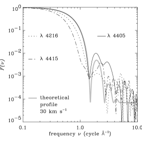
Figure 5: Example of line profiles in the Fourier space for HD 75063 (A1III type star) whose $v\sin i=30\,\mathrm{km}\,\mathrm{s}^{-1}$. The theoretical rotational profile (grey solid line), computed for the average $v\sin i$ of the star, matches perfectly the FT of the Fe i 4405 line (black solid line), whereas Fourier profiles of Sr ii 4216 and Fe i 4415 differ from a rotational shape. Among these three observed lines, only Fe i 4405 is retained for $v\sin i$ determination.

This comparison, carried out visually, allows us to discard non suitable Fourier profiles as shown in Fig. 5.

A discarded Fourier profile is sometimes associated with a distorted profile in wavelength space, but this is not always the case. For low rotational broadening, i.e. $v\sin i\lesssim 10$ $\mathrm{km}\,\mathrm{s}^{-1}$, the Fourier profile deviates from the theoretical rotational profile. This is due to the fact that rotation does not completely dominate the line profile and the underlying instrumental profile is no longer negligible. It may also occur that an SB2 system, where lines of both components are merged, appears as a single star, but the blend due to multiplicity makes the line profile diverge from a rotational profile.

To conclude, the number of measurable lines among the 15 listed in Table 2 also varies from one spectrum to another according to the rotational broadening and the signal-to-noise ratio and ranges from 1 to 15 lines.

Figure 6: Average number of measured lines (running average over 30 points) is plotted as a function of the mean $\langle v\sin i\rangle$.

As shown in Fig. 6, the average number of measured lines decreases almost linearly with increasing $v\sin i$, because of blends, and reaches one (the Mg ii 4481 doublet line) at $v\sin i\approx 100$ $\mathrm{km}\,\mathrm{s}^{-1}$. Below about 25 $\mathrm{km}\,\mathrm{s}^{-1}$, the number of measured lines decreases with $v\sin i$ for two reasons: first, Mg ii line is not used due to its intrinsic width; and more lines are discarded because of their non-rotational Fourier profile, instrumental profile being less negligible.

3.4 Systematic effect due to continuum

The measured continuum differs from the true one, and the latter is generally underestimated due to the wings of H$\gamma$ and the blends of weak metallic lines. One expects a systematic effect of the pseudo-continuum on the $v\sin i$ determination as the depth of a line appears lower, and so its FWHM.

We use the grid of synthetic spectra to derive rotational broadening from “true normalized” spectra (directly given by the models) and “pseudo normalized” spectra (normalized in the same way as the observed spectra). The difference of the two measurements is

$$\delta v\sin i=v\sin i-v\sin i^{\prime},$$ (5)

where $v\sin i$ is the rotational broadening derived using a pseudo-continuum and $v\sin i^{\prime}$ using the true continuum.

Figure 7: Systematic shift $\delta v\sin i$ as a function of the true rotational broadening $v\sin i^{\prime}$ for: a Fe i 4405 and b Mg ii 4481. The different symbols stand for the effective temperature of the synthetic spectra: fill circle: 10 000 K; square: 9200 K; diamond: 8500 K; triangle: 7500 K.

The systematic effect of the normalization induces an underestimation of the $v\sin i$ as shown in Fig. 7. This shift depends on the spectral line and its relative depth compared to the difference between true and pseudo-continuum. For Fe i 4405 (Fig. 7.a), the shift is about $0.15\,(v\sin i^{\prime}-30)$, which leads to large differences. The effect is quite uniform in temperature as reflected by the symmetric shape of the line all along the spectral sequence (Table 3). Nevertheless, at $v\sin i^{\prime}=150$ $\mathrm{km}\,\mathrm{s}^{-1}$, the scattering can be explained by the strength of H$\gamma$ whose wing is not negligible compared to the flattened profile of the line. For Mg ii 4481 (Fig. 7.b), the main effect is not due to the Balmer line but to blends of metallic lines. The shift remains small for early A-type stars (filled circles and open squares): $\lesssim 5$ %, but increases with decreasing effective temperature of the spectra, up to 10 %. This is due to the fact that Mg ii doublet is highly affected by blends for temperatures cooler than about 9000 K.

This estimation of the effect of the continuum is only carried out on synthetic spectra because the way our observed spectra have been normalized offers no way to recover the true continuum. The resulting shift is given here for information only.

3.5 Precision

Two types of uncertainties are present: those internal to the method and those related to the line profile.

The internal error comes from the uncertainty in the real position of the first zero due to the sampling in the Fourier space. The Fourier transforms are computed over 1024 points equally spaced with the step $\Delta\nu$. This step is inversely proportional to the step in wavelength space $\Delta\lambda$, and the spectra are sampled with $\Delta\lambda=0.05$ Å. The uncertainty of $v\sin i$ due to the sampling is

$$\begin{array}[]{ccl}\Delta v\sin i&\propto&(v\sin i)^{2}\,\lambda_{\mathrm{o}}\,\Delta\nu\\ &\propto&(v\sin i)^{2}\,{\lambda_{\mathrm{o}}\over\Delta\lambda}\\ &\approx&4.\,10^{-4}\,(v\sin i)^{2}.\end{array}$$ (6)

This dependence with $v\sin i$ to the square makes the sampling step very small for low $v\sin i$ and it reaches about 1 $\mathrm{km}\,\mathrm{s}^{-1}$ for $v\sin i=50$ $\mathrm{km}\,\mathrm{s}^{-1}$.

The best way to estimate the precision of our measurements is to study the dispersion of the individual $v\sin i$. For each star, $v\sin i$ is an average of the individual values derived from selected lines.

3.5.1 Effect of $v\sin i$

The error associated with the $v\sin i$ is expected to depend on $v\sin i$, because Doppler broadening makes the spectral lines shallow; that is, it reduces the contrast line/continuum and increases the occurrence of blends. Both effects tend to disrupt the selection of the lines as well as the access to the continuum. Moreover, the stronger the rotational broadening is, the fewer measurable lines there are. In Fig. 8, the differences between the individual $v\sin i$ values from each measured line in each spectrum with the associated mean value for the spectrum are plotted as a function of $\langle v\sin i\rangle$.

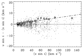
Figure 8: Differences between individual $v\sin i$ and mean over a spectrum $\langle v\sin i\rangle$. Variation of the standard deviation associated with the measure as a function of $\langle v\sin i\rangle$ is shown by the open circles. A linear least squares fit on these points (dot-dashed line) gives a slope of 0.06.

A robust estimate of the standard deviation is computed for each bin of 50 points; resulting points (open grey circles in Fig. 8) are adjusted with a linear least squares fit (dot-dashed line) giving:

$$\sigma_{v\sin i|v\sin i}=0.059{\scriptstyle\pm 0.003}\,\langle v\sin i\rangle.$$ (7)

The fit is carried out using GaussFit (Jefferys et al. 1998a, b), a general program for the solution of least squares and robust estimation problems. The formal error is then estimated as 6 % of the $v\sin i$ value.

3.5.2 Effect of spectral type

Figure 9: Mean of differences between individual $v\sin i$ and average $\langle v\sin i\rangle$ over a spectrum, normalized by the formal error due to $v\sin i$, are indicated for each spectral type by the open squares. The standard deviations of these means for each spectral class are plotted as filled circles, with their associated error bar.

Residual around this formal error can be expected to depend on the effective temperature of the star. Figure 9 displays the variations of the residuals as a function of the spectral type. Although contents of each bin of spectral type are not constant all across the sample (the error bar is roughly proportional to the logarithm of the inverse of the number of points), there does not seem to be any trend, which suggests that our choice of lines according to the spectral type eliminates any systematic effect due to the stellar temperature from the measurement of the $v\sin i$.

3.5.3 Effect of noise level

Although noise is processed as a high frequency signal by Fourier technique and not supposed to act much upon $v\sin i$ determination from the first lobe of the FT, signal-to-noise ratio (SNR) may affect the measurement. SNR affects the choice of the lines’ limits in the spectrum as well as the computation of the lines’ central wavelength.

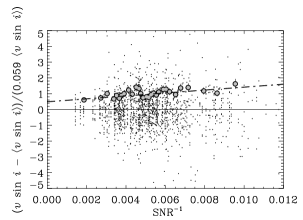
Figure 10: Differences between individual $v\sin i$ and mean over a spectrum $\langle v\sin i\rangle$, normalized by the formal error due to $v\sin i$. Variation of the standard deviation associated to the measure with the noise level (SNR^-1) is shown by the open circles. A linear least squares fit on these points (dot-dashed line) gives a slope of $\sim 100$

The differences $v\sin i-\langle v\sin i\rangle$, normalized by the formal error $0.059\,\langle v\sin i\rangle$, are plotted versus the noise level (SNR^-1) in Fig. 10 in order to estimate the effect of SNR. Noise is derived for each spectrum using a piecewise-linear high-pass filter in Fourier space with a transition band chosen between $0.3$ and $0.4$ times the Nyquist frequency; standard deviation of this high frequency signal is computed as the noise level and then divided by the signal level. The trend in Fig. 10 is computed as for Fig. 8, using a robust estimation and GaussFit. The linear adjustment gives:

$$\hat{\sigma}_{v\sin i|\mathrm{SNR}}=93{\scriptstyle\pm 16}\,\mathrm{SNR}^{-1}+0.5{\scriptstyle\pm 0.1}.$$ (8)

The distribution of mean signal-to-noise ratios for our observations peaks at $\mathrm{SNR}=190$ with a standard deviation of $78$. This means that for most of the observations, SNR does not contribute much to the formal error on $v\sin i$ ($\hat{\sigma}_{v\sin i|\mathrm{SNR}}\approx 1$). Finally, the formal error associated with the $v\sin i$ can be quantified as:

$$\begin{array}[]{ccl}\sigma_{v\sin i}&=&\sigma_{v\sin i|v\sin i}\,\hat{\sigma}_{v\sin i|\mathrm{SNR}}\\ &=&\left(0.059\,\langle v\sin i\rangle\right)\,\left(93\,\mathrm{SNR}^{-1}+0.5\right)\\ &\propto&{v\sin i\over\mathrm{SNR}}.\end{array}$$ (9)

3.5.4 Error distribution

Distribution of observational errors, in the case of rotational velocities, is of particular interest during a deconvolution process in order to get rid of statistical errors in a significant sample.

To have an idea of the shape of the error law associated with the $v\sin i$, it is necessary to have a great number of spectra for the same star. Sirius has been observed on several occasions during the runs and its spectrum has been collected 48 times. Sirius spectra typically exhibit high signal-to-noise ratio (SNR $\gtrsim 250$). The 48 values derived from each set of lines, displayed in Fig. 11, give us an insight into the errors distribution. The mean $v\sin i$ is $16.22{\scriptstyle\pm 0.04}$ $\mathrm{km}\,\mathrm{s}^{-1}$ and its associated standard deviation $0.27{\scriptstyle\pm 0.03}$ $\mathrm{km}\,\mathrm{s}^{-1}$; data are approximatively distributed following a gaussian around the mean $v\sin i$.

Figure 11: The $v\sin i$ determinations for the 48 spectra of Sirius are distributed around the mean $16.22{\scriptstyle\pm 0.04}$ $\mathrm{km}\,\mathrm{s}^{-1}$ with a dispersion of $0.27{\scriptstyle\pm 0.03}$ $\mathrm{km}\,\mathrm{s}^{-1}$. The optimal normal distribution $\mathscr{N}(16.23,0.21)$ that fits the histogram with a 96 % significance level is over-plotted. The optimal log-normal distribution merges together with the gaussian.

A Kolmogorov-Smirnov test shows us that, with a 96 % significance level, this distribution is not different from a gaussian centered at 16.23 with a standard deviation equal to 0.21. In the case of Sirius (low $v\sin i$) the error distribution corresponds to a normal distribution. We may expect a log-normal distribution as the natural error law, considering that the error on $v\sin i$ is multiplicative. But for low $v\sin i$, and low dispersion, log-normal and normal distributions do not significantly differ from each other.

Moreover, for higher broadening, the impact of the sampling effect of the FT (Eq. 6) is foreseen, resulting in a distribution with a box-shaped profile. This effect becomes noticeable for $v\sin i\gtrsim 100$ $\mathrm{km}\,\mathrm{s}^{-1}$.

4 Rotational velocities data

4.1 Results

In all, projected rotational velocities were derived for 525 B8 to F2-type stars. Among them, 286 have no rotational velocities either in the compilation of Uesugi & Fukuda (1982) or in Abt & Morrell (1995).

The results of the $v\sin i$ determinations are presented in Table 4 which contains the following data: column (1) gives the HD number, column (2) gives the HIP number, column (3) displays the spectral type as given in the HIPPARCOS catalogue (ESA 1997), columns (4,5,6) give respectively the derived value of $v\sin i$, the associated standard deviation and the corresponding number of measured lines (uncertain $v\sin i$ are indicated by a colon), column (7) presents possible remarks about the spectra: SB2 (“SB”) and shell (“SH”) natures are indicated for stars detailed in the subsections which follow, as well as the reason why $v\sin i$ is uncertain – “NO” for no selected lines, “SS” for variation from spectrum to spectrum and “LL” for variation from line to line, as detailed in the Appendix A.

Grenier et al. (1999) studied the same stars with the same spectra and derived radial velocities using cross-correlation techniques. On the basis of the shape of the cross-correlation function (CCF) they find that less than half of the sample has a symmetric and gaussian CCF and they classify stars with distorted CCF as, among other things, “certain” “probable” or “suspected” doubles.

Table 4: (extract) Results of the $v\sin i$ measurements. Only the 15 first stars are listed below. The whole table is available electronically.

HD	HIP	Spect. type	$v\sin i$	$\sigma$	#	Remark
			($\mathrm{km}\,\mathrm{s}^{-1}$)
256	602	A2IV/V	243	9	2
319	636	A1V	61	5	8
560	813	B9V	249	–	1
565	798	A6V	149	0	2
1064	1191	B9V	128	–	1
1685	1647	B9V	236	–	1
1978	1900	A0	110:	–	1	NO
2696	2381	A3V	168	3	2
3003	2578	A0V	93	–	1
3652	3090	F0	46	–	1
4065	3356	B9.5V	35	4	4
4125	3351	A6V	90	–	1
4150	3405	A0IV	124	0	2
4338	3576	F0IV	75	–	1
4772	3858	A3IV	157	3	2

Uncertainties in $v\sin i$ are induced by peculiarities in the spectra due for example to binarity or to the presence of a shell. The results for these objects are detailed below. These objects were either known as binaries or newly detected by Grenier et al. (1999).

4.1.1 Binary systems

Spectra of double-lined spectroscopic binary systems (SB2) display lines of both components of the system. They are, by nature, more affected by blends and require much more attention than single stars in order to disentangle both spectra.

Moreover, the difference in radial velocity $\Delta V_{\mathrm{r}}$ has to be large enough for the spectrum to show well separated lines. Considering a gaussian line profile, 98 % of the distribution is contained between $\pm 2.326\,\sigma$ ($\sigma$ being the standard deviation of the Gaussian) which is nearly equal to $\pm\mathrm{FWHM}$. It follows that a double line resulting from the contribution of the components of a binary system should be spaced of $|\Delta\lambda_{\mathrm{A}}-\Delta\lambda_{\mathrm{B}}|\gtrsim 2\,\mathrm{FWHM}$ (where $\Delta\lambda_{\mathrm{A}}$ and $\Delta\lambda_{\mathrm{B}}$ are the respective Doppler shifts) to overlap as little as possible and be measurable in terms of $v\sin i$ determination. Taking the calibration relation from SCBWP as a rule of thumb ($\mathrm{FWHM}{\scriptstyle[\mathrm{\AA}]}\approx 0.025\,v\sin i{\scriptstyle[\mathrm{km}\,\mathrm{s}^{-1}]}$), the difference of radial velocity in an SB2 system should be higher than:

$$\Delta V_{\mathrm{r}}\gtrsim{2\,c\,0.025\over\lambda}\,v\sin i\approx 3.4\,v\sin i,$$ (10)

where $c$ is the velocity of light and $\lambda$ the wavelength of the line ($\sim 4350$ Å). This threshold is a rough estimate of whether $v\sin i$ is measurable in the case of SB2. On the other hand, the respective cores of the double line cease to be distinct when relative Doppler shift is lower than the FWHM, considering gaussian profiles, i.e. $\Delta V_{\mathrm{r}}\lesssim 1.1\,v\sin i$. Below this value, lines of both components merge.

Figure 12: The part of the spectrum of HD 10167, centered around Mg ii 4481 (4460–4500 Å) is displayed for the two observed spectra of the star. Both panels present the binarity. Relative radial velocities are high enough compared to rotational broadening to allow to measure $v\sin i$ for both components. Observation b occurs nearly two years after observation a.

Figure 13: HD 18622 has been observed at three different times: a HJD 2 447 790, b 2 448 525 and c 2 448 584. For each spectrum the region around Mg ii 4481 Å is displayed. Relative radial velocities vary from about indiscernible components in panel c to nearly 150 $\mathrm{km}\,\mathrm{s}^{-1}$ in a. Relatively high rotational broadening makes the measurement of $v\sin i$ difficult because of the ratio $\Delta V_{\mathrm{r}}\over v\sin i$, and derived rotational velocities are uncertain.

Figure 14: HD 27346 spectra have been collected at two different orbital phases separated in time by 981 days. Mg ii line shows clearly the two components in panel a, whereas they are merged in b.

Figure 15: a and b Observations of HD 87330 around Mg ii, separated by almost three years. Low rotational broadening allows the measurement of $v\sin i$ using weak metallic lines, whereas Mg ii line of both components overlap, due to the intrinsic width of the doublet. c Spectrum of the late B star HD 90972, with few metallic lines. The low difference of radial velocities makes the measurement of $v\sin i$ uncertain.

Table 5 displays the results for the stars in our sample which exhibit an SB2 nature. We focus only on stars in which the spectral lines of both component are separated. Spectral lines are identified by comparing the SB2 spectrum with a single star spectrum. Projected rotational velocities are given for each component when measurable, as well as the difference in radial velocity $\Delta V_{\mathrm{r}}$ computed from the velocities given by Grenier et al. (1999).

Table 5: Results of the $v\sin i$ measurements for individual spectra of SB2 systems. When available, the $v\sin i$ measurements are given for each component (A for the bluest and B for the reddest). The difference of radial velocity is also given, derived from Grenier et al. Dash (–) indicates a non-determined value: no double-peak CCF for $\Delta V_{\mathrm{r}}$ measurement, and $1.1\,v\sin i\lesssim\Delta V_{\mathrm{r}}\lesssim 3.4\,v\sin i$ for individual $v\sin i$ measurement. When SB2 signature is not detectable a single $v\sin i$ of merged lines is measured. Last column refers to the corresponding figures.

HD	HIP	Spect. type	$v\sin i$		$\Delta V_{\mathrm{r}}$	Fig.
			($\mathrm{km}\,\mathrm{s}^{-1}$)		($\mathrm{km}\,\mathrm{s}^{-1}$)
			A	B
10167	7649	F0V	17	14	80	12a.
			11	13	62	12b.
18622	13847	A4III+…	71:	74:	154	13a.
			–	–	109	13b.
			83		–	13c.
27346	19704	A9IV	35	35	135	14a.
			36:		–	14b.
87330	49319	B9III/IV	11	9	67	15a.
			10	10	45	15b.
90972	51376	B9/B9.5V	23:	29:	54	15c.

• HD 10167 has given no indication of a possible duplicity up to now in the literature and is used as a photometric standard star (Cousins 1974).

• HD 18622 ($\theta^{1}$ Eri) is a binary system for which HIPPARCOS measured the angular separation $\rho=8\aas@@fstack{\prime\prime}31{\scriptstyle\pm 0.003}$ and the difference of magnitude $\Delta Hp=1.09{\scriptstyle\pm 0.01}$ of the visual system, while our data concern the SB2 nature of the primary.

• HD 27346 is suspected to be an astrometric binary on the basis of HIPPARCOS observations.

• HD 87330 was detected as a variable star by HIPPARCOS and its variability is possibly due to duplicity.

• HD 90972 ($\delta$ Ant) is a visual double system (Pallavicini et al. 1992) whose primary is an SB2 for which the $v\sin i$ of both components are given in Table 5. Grenier et al. do not identify $\delta$ Ant as an SB2 system but point to it as a certain double star on the basis of the CCF. It is worth noticing that their CCF is equivalent to a convolution with observed and synthetic spectra and the resulting profile is smoothed by both.

The magnesium doublet is perfectly suited to distinguish a spectral duplicity, so that spectral domain around 4481 Å is displayed for SB2 systems is Figs. 12, 13, 14, 15. However, the intrinsic width of the doublet increases its blend due to multiplicity whereas fainter lines can be clearly separated, and Mg ii line is not used to derive $v\sin i$ for SB2 systems.

Less obvious SB2 lie in our sample, but individually analyzing line profiles one-by-one is not an appropriate method for detecting them. Results about binarity for these spectra are however indicated in Grenier et al.

4.1.2 Metallic shell stars

The specific “shell” feature in stars with a circumstellar envelope is characterized by double emission and central absorption in hydrogen lines. This characteristic is likely a perspective effect, as suggested by Slettebak (1979), and shell-type lines occur at high inclination $i$ when line of sight intersects with the disk-like envelope. For our purpose, $v\sin i$ determination, critical effect is due to metallic shell stars, where shell-type absorption not only occurs in Balmer series but also in metallic lines. Our candidate lines exhibit a broad profile, indicating rapid rotation of the central star, a high inclination of the line of sight, and a superimposed sharp absorption profile originating in the circumstellar envelope (Fig. 16). Metallic shell-type lines arise when perspective effect is more marked than for hydrogen shell stars (Briot 1986). Measurement of $v\sin i$ requires a line profile from the central star photosphere only, and not polluted by absorption caused by the circumstellar envelope which does not reflect the rotation motion.

Figure 16: Part of the spectrum of HD 225200 showing the rotationally broadened line Mg ii 4481 (filled circle) and metallic lines exhibiting the signature of the shell as sharp core and extended wings (open triangle).

Derived $v\sin i$ for the metallic shell stars present in our sample are listed in Table 6. These stars are already known as shell stars. HD 15004 (71 Cet) and HD 225200 are further detailed by Gerbaldi et al. In our spectral range, magnesium multiplet Mg ii 4481 is the only measurable line.

Table 6: Results of the $v\sin i$ measurements for individual spectra of metallic shell stars.

HD	HIP	Spectral type	$v\sin i$
			($\mathrm{km}\,\mathrm{s}^{-1}$)
15004	11261	A0III	249
24863	18275	A4V	249
38090	26865	A2/A3V	204
88195	49812	A1V	236
99022	55581	A4:p	236
			236
			249
225200	345	A1V	345

4.2 Comparison with existing data

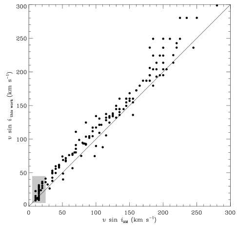
Figure 17: Comparison between $v\sin i$ values from this work and from Abt & Morrell (1995, AM) for the 160 common stars. The solid line stands for the one-to-one relation. The grey box encompasses the points of low $v\sin i$, for which the relation has a much higher local slope and produces an overestimation of the global slope.

Figure 18: Comparison between $v\sin i$ data from this work and from Slettebak et al. The solid line stands for the one-to-one relation. The 35 standard stars are plotted with error bar on both axes (see text). The stars that deviate most from the one-to-one relation have their HD number indicated and are summarized in Table 7.

The most homogeneous large data set of rotational velocities for A-type stars which has been provided up to now is that of Abt & Morrell (1995), who measured $v\sin i$ for about 1700 A-type stars in the northern hemisphere. The intersection with our southern sample includes 160 stars. The comparison of the $v\sin i$ (Fig. 17) shows that our determination is higher on average than the velocities derived by Abt & Morrell (AM). The linear relation given by GaussFit is:

$$v\sin i_{\mathrm{this\;work}}=1.15{\scriptstyle\pm 0.03}\,v\sin i_{\mathrm{AM}}+2.1{\scriptstyle\pm 0.8}.$$ (11)

Abt & Morrell based their measurements on the scale established by SCBWP, who built a new calibration FWHM-$v\sin i$, replacing the old system and leading to values 5 % smaller on average for A-F stars.

There are 35 stars in common between our sample and the standard stars of SCBWP. It is worth emphasizing that among these 35 stars, only one third has a gaussian CCF in the study of Grenier et al. Moreover there is an SB2 system (HD 18622) and almost one half of this group is composed of suspected or probable multiple stars, on the basis of their CCF.

Figure 18 displays the $v\sin i$ derived in this paper versus the $v\sin i$ from SCBWP for the 35 standard stars in common. The solid line represents the one-to-one relation. A clear trend is observed: $v\sin i$ from SCBWP are on average 10 to 12 % lower. A linear least squares fit carried out with GaussFit on these values makes the systematic effect explicit:

$$v\sin i_{\mathrm{this\;work}}=1.04{\scriptstyle\pm 0.02}\,v\sin i_{\mathrm{SCBWP}}+6.1{\scriptstyle\pm 1.0}.$$ (12)

The relation is computed taking into account the error bars of both sources. The error bars on the values of SCBWP are assigned according to the accuracy given in their paper (10 % for $v\sin i<200\,\mathrm{km}\,\mathrm{s}^{-1}$ and 15% for $v\sin i\geq 200\,\mathrm{km}\,\mathrm{s}^{-1}$). Our error bars are derived from the formal error found in section 3.5 (Eq. 9).

The difference between the two relations, (Eq. 11) and (Eq. 12), concerns mainly the low $v\sin i$ region. When low $v\sin i$ from Abt & Morrell, $<25$ $\mathrm{km}\,\mathrm{s}^{-1}$, are not taken into account (grey box in Fig. 17), the relation given by GaussFit between $v\sin i$ from Abt & Morrell and this work becomes:

$$v\sin i_{\mathrm{this\;work}}=1.08{\scriptstyle\pm 0.02}\,v\sin i_{\mathrm{AM}}+5.3{\scriptstyle\pm 1.8},$$ (13)

which is almost identical to the relation with SCBWP data (Eq. 12).

Table 7: Highlight of the discrepancy between $v\sin i$ values from SCBWP and ours (standard deviation of our measurement is indicated; dash “–” stands for only one measurement). Comparison with data from the literature for the twelve stars that exhibit the largest differences. $v\sin i$ are classified in three subgroups according to the way they are derived: by-product of a spectrum synthesis, frequency analysis of the lines profiles or infered from a FWHM-$v\sin i$ relation independent from SCBWP’s one. Flags from HIPPARCOS catalogue are indicated: variability flag H52 (C: constant, D: duplicity-induced variability, M: possibly micro-variable, U: unsolved variable, –: no certain classification) and double annex flag H59 (O: orbital solution, G: acceleration terms, –: no entry in the Double and Multiple Systems Annex). The shape of the CCF found by Grenier et al. is also given (0: symmetric and gaussian peak, 1: SB2, 2: certain double, near spectral types, 3: certain double, A-B type with faint F-G component, 4: probable double, 5: suspected double, 6: probable multiple system, 7: certain shell star, 8: suspected shell star, 9: wide and irregular peak, 10: wide peak of B star (few lines)).

Name	HD	Sp. type	$v\sin i$ ($\mathrm{km}\,\mathrm{s}^{-1}$)						hipparcos		CFF
			scbwp	this work		literature			H52	H59
						spec. synth.	freq. analysis	FWHM
$\eta$ Phe	4150	A0IV	$105$	$124$	${\scriptstyle\pm 0}$	–	–	–	C	G	4
$\nu$ Pup	47670	B8III	$200$	$246$	${\scriptstyle\pm 7}$	–	–	–	U	–	5
$\alpha$ CMa	48915	A0m…	$10$	$16$	${\scriptstyle\pm 1}$	$16{\scriptstyle\pm 1}^{(1)}\;16^{(2)}$	$17^{(4)}\;16.9^{(5)}$	–	–	–	0
						$16.2^{(3)}$	$19^{(6)}\;15.3{\scriptstyle\pm 0.3}^{(7)}$
$QW$ Pup	55892	F0IV	$40$	$51$	${\scriptstyle\pm 8}$	–	–	$50^{(8)}$	M	–	4
$a$ Vel	75063	A1III	$20$	$30$	${\scriptstyle\pm 2}$	–	–	–	–	–	0
$\alpha$ Vol	78045	Am	$25$	$34$	${\scriptstyle\pm 2}$	$45^{(9)}$	–	–	C	–	0
$\theta$ Leo	97633	A2V	$15$	$23$	${\scriptstyle\pm 1}$	$21^{(2)}\;22.1^{(3)}$	–	$23^{(10)}$	–	–	0
$A$ Cen	100673	B9V	$125$	$160$	–	–	–	–	C	–	10
$\lambda$ Mus	102249	A7III	$50$	$60$	${\scriptstyle\pm 2}$	–	–	$60^{(11)}$	C	O	0
$\psi$ Cen	125473	A0IV	$100$	$124$	${\scriptstyle\pm 2}$	$132^{(9)}$	–	–	–	–	5
$\epsilon$ Aqr	198001	A1V	$85$	$102$	–	$108.1^{(3)}\;95^{(12)}$	–	–	–	–	0
$\omega^{2}$ Aqr	222661	B9V	$120$	$150$	–	–	–	–	C	–	4

(1) Kurucz et al. (1977)	(5) Deeming (1977)	(9) Holweger et al. (1999)
(2) Lemke (1989)	(6) Ramella et al. (1989)	(10) Fekel (1998)
(3) Hill (1995)	(7) Dravins et al. (1990)	(11) Noci et al. (1984)
(4) Smith (1976)	(8) Balachandran (1990)	(12) Dunkin et al. (1997)

For slow rotational velocities, the discrepancy far exceeds the estimate of observational errors. Figure 18 also shows the stars which deviate the most from the one-to-one relation. These twelve stars, for which the error box around the point does not intersect with the one-to-one relation, are listed in Table 7 with different rotational velocity determinations gathered from the literature. Their large differences together with comparison to other data allow us to settle on which source carries the systematic effect. Without exception, all data gathered from the literature and listed in Table 7 are systematically higher than the corresponding SCBWP’s $v\sin i$ and for the majority of the listed stars, data from the literature are consistent with our $v\sin i$ determinations. These stars are further detailed in the Appendix B.

5 Discussion and conclusion

The selection of several suitable spectral lines and the evaluation of their reliability as a function of broadening and effective temperature allows the computation of $v\sin i$ over the whole spectral range of A-type stars and a robust estimate of the associated relative error.

Up to 150 $\mathrm{km}\,\mathrm{s}^{-1}$, a statistical analysis indicates that the standard deviation is about 6 % of the $v\sin i$. It can be seen, in both Figs. 17 and 18, that the dispersion increases beyond 180 $\mathrm{km}\,\mathrm{s}^{-1}$ approximately, when comparing rotational velocities to previous determination by Abt & Morrell and SCBWP. SCBWP estimate a larger uncertainty for rotational velocities higher than 200 $\mathrm{km}\,\mathrm{s}^{-1}$; nevertheless our precision estimation for a 200 $\mathrm{km}\,\mathrm{s}^{-1}$ $v\sin i$ is extrapolated from Fig. 8. Errors may thus be larger, due to the sampling in Fourier space, which is proportional to $(v\sin i)^{2}$.

In addition, determination of continuum level induces a systematic underestimation of $v\sin i$ that reaches about 5 to 10 % depending on the lines and broadening.

Gravity darkening (von Zeipel effect, von Zeipel 1925) is not taken into account in this work. Hardorp & Strittmatter (1968) quantify this effect, showing that $v\sin i$ could be 15 to 40 % too small if gravity darkening is neglected for stars near break-up velocity. Nevertheless, in a recent work (Shan 2000), this effect is revised downwards and found to remain very small as long as angular velocity is not close to critical velocity ($\omega<0.8$): it induces an underestimation lower than 1 % of the FWHM. In our observed sample, 15 stars (with spectral type from B8V to A1V) have $v\sin i>250$ $\mathrm{km}\,\mathrm{s}^{-1}$. According to their radii and masses, derived from empirical calibrations (Habets & Heintze 1981), their critical velocities $v_{\mathrm{c}}$ are higher than 405 $\mathrm{km}\,\mathrm{s}^{-1}$ (Zorec, private communication). Only seven stars have a high $v\sin i$, so that $v\sin i/v_{\mathrm{c}}>0.7$. The fraction of stars rotating near their break-up velocity remains very small, probably lower than 2 % of the sample size.

A systematic shift is found with the values from the catalogue of Abt & Morrell (1995). This difference arises from the use of the calibration relation from SCBWP, for which a similar shift is found. The discrepancy observed with standard $v\sin i$ values given by SCBWP has already been mentioned in the literature. Ramella et al. (1989) point out a similar shift with respect to the $v\sin i$ from SCBWP. They suppose that the discrepancy could come from the models SCBWP used to compute theoretical FWHM of the Mg ii line. Brown & Verschueren (1997) derived $v\sin i$ for early-type stars. For low $v\sin i$ (up to $\sim 60$ $\mathrm{km}\,\mathrm{s}^{-1}$), their values are systematically higher than those of SCBWP. They attribute this effect to the use of the models from Collins & Sonneborn (1977) by SCBWP; they assert that using the modern models of Collins et al. (1991), to derive $v\sin i$ from FWHM, eliminates the discrepancy. Fekel (private communication) also finds this systematic effect between values from Abt & Morrell (1995), which are directly derived from the SCBWP’s calibration, and the $v\sin i$ he measured using his own calibration (Fekel 1997).

In addition, some stars used as $v\sin i$ standards turn out to be multiple systems or to have spectral features such that their status as a standard is no longer valid. The presence of these “faulty” objects in the standard star sample may introduce biases in the $v\sin i$ scale. There is no doubt that the list of standards established by SCBWP has to be revised.

The above comparisons and remarks lead us to call into question the $v\sin i$ values of the standard stars from SCBWP.

This paper is a first step, and a second part will complete these data with a northern sample of A-type stars.

Appendix A notes on stars with uncertain rotational velocity

A.1 Stars with no selected line

For a few spectra, all the measurable lines were discarded either a priori from Table 3 or a posteriori because of a distorted FT. These stars appear in Table 4 with an uncertain $v\sin i$ (indicated by a colon) and a flag “NO”. They are detailed below:

• HD 1978 is rapid rotator whose Mg ii line FT profile is distorted ($v\sin i=110:$ $\mathrm{km}\,\mathrm{s}^{-1}$).

• HD 41759, HD 93905 and HD 99922 have a truncated spectrum: only two thirds of the spectral range are covered (from 4200 to 4400 Å). Half of the selected lines are thus unavailable and estimation of the $v\sin i$ is then given, as an indication, by lines that would have normally been discarded by the high skewness of their synthetic profile. ($v\sin i=215:,\;85:,\;65:$ $\mathrm{km}\,\mathrm{s}^{-1}$ respectively)

• HD 84121 is a sharp-lined A3IV star ($v\sin i=10:$ $\mathrm{km}\,\mathrm{s}^{-1}$). It is resolved by HIPPARCOS as a binary system (separation $0\aas@@fstack{\prime\prime}125\,\pm 0\aas@@fstack{\prime\prime}006$ and magnitude difference $\Delta Hp=0.61\pm 0.31$ mag) and highly suspected to hide a third component (Söderhjelm 1999).

• HD 103516 is a supergiant A3Ib star ($v\sin i=20:$ $\mathrm{km}\,\mathrm{s}^{-1}$).

• HD 111786 is detected binary by Faraggiana et al. (1997) ($v\sin i=45:$ $\mathrm{km}\,\mathrm{s}^{-1}$).

• HD 118349 is a A7-type star indicated as variable in photometry, due to duplicity, by HIPPARCOS ($v\sin i=100:$ $\mathrm{km}\,\mathrm{s}^{-1}$).

A.2 Stars with high external error

The following stars have a mean $v\sin i$ whose associated standard deviation is higher than 15 % of the $v\sin i$. This dispersion may either come from differences from one spectrum to another or lie in a single spectrum.

Some of the stars whose spectrum has been collected several times show different $v\sin i$ from one spectrum to another (flag “SS” in Table 4). These differences could be related to intrinsic variations in the spectrum itself. Other stars present a high dispersion in the measures from lines in a single spectrum (flag “LL” in Table 4). These stars are detailed in appendices A.2.1 and A.2.2 respectively.

A.2.1 Variations from spectrum to spectrum

• HD 55892 has two very different $v\sin i$ derived from its two collected spectra : 45 and 56 $\mathrm{km}\,\mathrm{s}^{-1}$. Probable double in Grenier et al. (1999).

• HD 74461 $73\,\mathrm{km}\,\mathrm{s}^{-1}\pm 15\,\mathrm{km}\,\mathrm{s}^{-1}$ and $93\,\mathrm{km}\,\mathrm{s}^{-1}\pm 6\,\mathrm{km}\,\mathrm{s}^{-1}$. Probable double in Grenier et al. (1999).

• HD 87768 shows two different values in the two spectra: 90 and 112 $\mathrm{km}\,\mathrm{s}^{-1}$. It is indicated as a certain double star by Grenier et al. (1999), whose primary is an A star and secondary should be a faint F-G star. Abt & Willmarth (1994), point to it as an SB2 system on the basis of the study of its radial velocity.

• HD 174005 has two very different $v\sin i$ derived from its two collected spectra ($129\pm 5$ and $66\pm 7$ $\mathrm{km}\,\mathrm{s}^{-1}$). It is classified as a certain double star, with components of similar spectral types, by Grenier et al. (1999).

• HD 212852 shows two different values in the two spectra: 93 and 121 $\mathrm{km}\,\mathrm{s}^{-1}$. It is suspected double by Grenier et al. (1999).

A.2.2 Variations from line to line

• HD 40446 is a A1Vs star whose $v\sin i$ is found as $27\pm 5$ $\mathrm{km}\,\mathrm{s}^{-1}$. The stochastic motion solution in HIPPARCOS data may suggest a possible multiplicity.

• HD 109074 is a A3V star with $v\sin i=84\pm 15$ $\mathrm{km}\,\mathrm{s}^{-1}$. HIPPARCOS astrometric solution comprises acceleration terms, which could indicate a multiplicity.

Appendix B notes on $v\sin i$ standard stars with discrepant rotational velocity

Standard stars from SCBWP that are listed in Table 7, are now detailed:

• $η$~Phe (HD 4150) is among the A0 dwarf stars investigated by Gerbaldi et al. (1999). They suspect $\eta$ Phe to be a binary system on the basis of the fit between the observed and the computed spectrum, as do Grenier et al. on the basis of the CCF of the spectrum.

• $ν$~Pup (HD 47670) is a late B giant star. It is part of the sample studied by Baade (1989a, b) who searches for line profile variability. He detects roughly central quasi-emission bumps in the rotationally broadened Mg ii absorption line. This feature could be caused by the change in effective gravity from equator to poles and the associated temperature differences because of fast rotation. Rivinius et al. (1999) tone down this result but conclude nevertheless that there is strong evidence that this star is a not previously recognized bright Be star. $\nu$ Pup was suspected to be a $\beta$ Cephei star (Shaw 1975) and is newly-classified as an irregular variable on the basis of the HIPPARCOS photometric observations.

• Sirius ($\alpha$ CMa, HD 48915) has a $v\sin i=10$ $\mathrm{km}\,\mathrm{s}^{-1}$ in the catalogue of SCBWP. Several authors have given larger values derived from approximatively the same spectral domain. Smith (1976) finds 17 $\mathrm{km}\,\mathrm{s}^{-1}$ and Kurucz et al. (1977) 16 $\mathrm{km}\,\mathrm{s}^{-1}$ $\pm 1$ $\mathrm{km}\,\mathrm{s}^{-1}$. Deeming (1977), using Bessel functions, finds 16.9 $\mathrm{km}\,\mathrm{s}^{-1}$. Lemke (1989), analyzing abundance anomalies in A stars, derives the $v\sin i$ of Sirius as an optimum fit over the spectral range: 16 $\mathrm{km}\,\mathrm{s}^{-1}$. Dravins et al. (1990) using Fourier techniques on high resolution and high signal-to-noise ratio spectra give 15.3 $\mathrm{km}\,\mathrm{s}^{-1}$ $\pm 0.3$ $\mathrm{km}\,\mathrm{s}^{-1}$. Hill (1995) studies a dozen A-type stars using spectral synthesis techniques to make an abundance analysis; fitting the spectra (four 65 Å wide spectral regions between 4500 and 5000 Å) he finds 16.2 $\mathrm{km}\,\mathrm{s}^{-1}$ as the $v\sin i$ of Sirius.

• $QW$~Pup (HD 55892) is an early F-type star. It belongs to the $\gamma$ Dor class of pulsating variable stars (Kaye et al. 1999). Balachandran (1990), studying lithium depletion, determines Li abundances and rotational velocities for a sample of nearly 200 F-type stars. Using her own FWHM–$v\sin i$ calibration, she finds 50 $\mathrm{km}\,\mathrm{s}^{-1}$ for $QW$ Pup, which gets closer to our determination. HIPPARCOS results show that $QW$ Pup is a possible micro-variable star.

• $a$~Vel (HD 75063) in an early A-type star. It is part of the sample of IRAS data studied by Tovmassian et al. (1997) in the aim of detecting circumstellar dust shells. They do not rule out that $a$ Vel may have such a feature. No relevant $v\sin i$ data have been found for this star.

• $α$~Vol (HD 78045) is a dusty A star on the basis of IRAS data (Cheng et al. 1992). Holweger et al. (1999) measure a $v\sin i$ significantly larger than the $v\sin i$ from SCBWP and even our determination.

• $θ$~Leo (HD 97633) is a candidate constant velocity A star. Fekel (1998) monitors it and attributes to it a $v\sin i=23\,\mathrm{km}\,\mathrm{s}^{-1}$. Lemke (1989) and Hill (1995) respectively measured it at 21 and 22.1 $\mathrm{km}\,\mathrm{s}^{-1}$. These values are significantly higher than 15 $\mathrm{km}\,\mathrm{s}^{-1}$ found by SCBWP.

• $A$~Cen (HD 100673) is a B-type emission line star.

• $λ$~Mus (HD 102249) has been measured by Noci et al. (1984) who derive its $v\sin i$ using the CCF and a calibration as described in Stauffer et al. (1984). In HIPPARCOS data, $\lambda$ Mus is a binary star for which orbital parameters are given: period $P=453\,\mathrm{d}\pm 8$ d, inclination $i=134\,\degr\pm 8$ °, semi-major axis of photocentre orbit $a_{0}=6.31\,\mathrm{mas}\pm 1.05$ mas.

• $ψ$~Cen (HD 125473) is a dusty A-star (Cheng et al. 1992). The rotational velocity derived by Holweger et al. (1999) agrees with our determination, 30 % larger than SCBWP.

• $ϵ$~Aqr (HD 198001) has a $v\sin i=85$ $\mathrm{km}\,\mathrm{s}^{-1}$ according to SCBWP, much smaller than the value in this work. The velocity derived by Hill is consistent with ours, taking into account the uncertainty of the measurements. Dunkin et al. (1997) found 95 $\mathrm{km}\,\mathrm{s}^{-1}$ by fitting the observed spectrum with a synthetic one.

• $ω^2$~Aqr (HD 222661) has, to our knowledge, no further determination of the $v\sin i$, independent of the SCBWP’s calibration.

References

- Abt & Morrell (1995) Abt, H. A. & Morrell, N. I. 1995, ApJS, 99, 135
- Abt & Willmarth (1994) Abt, H. A. & Willmarth, D. W. 1994, ApJS, 94, 677
- Baade (1989a) Baade, D. 1989a, A&AS, 79, 423
- Baade (1989b) —. 1989b, A&A, 222, 200
- Balachandran (1990) Balachandran, S. 1990, ApJ, 354, 310
- Briot (1986) Briot, D. 1986, A&A, 163, 67
- Brown & Verschueren (1997) Brown, A. G. A. & Verschueren, W. 1997, A&A, 319, 811
- Burnage & Gerbaldi (1990) Burnage, R. & Gerbaldi, M. 1990, in Data Analysis Workshop - 2nd ESO/ST-ECF Garching, 137
- Burnage & Gerbaldi (1992) Burnage, R. & Gerbaldi, M. 1992, in Data Analysis Workshop - 4th ESO/ST-ECF Garching, 159
- Carroll (1933) Carroll, J. A. 1933, MNRAS, 93, 478
- Cheng et al. (1992) Cheng, K.-P., Bruhweiler, F. C., Kondo, Y., & Grady, C. A. 1992, ApJ Lett., 396, L83
- Collins & Sonneborn (1977) Collins, G. W. I. & Sonneborn, G. H. 1977, ApJS, 34, 41
- Collins et al. (1991) Collins, G. W. I., Truax, R. J., & Cranmer, S. R. 1991, ApJS, 77, 541
- Cousins (1974) Cousins, A. W. J. 1974, Mon. Notes Astron. Soc. S. Afr., 33, 149
- Danziger & Faber (1972) Danziger, I. J. & Faber, S. M. 1972, A&A, 18, 428
- Deeming (1977) Deeming, T. J. 1977, Ap&SS, 46, 13
- Dravins et al. (1990) Dravins, D., Lindegren, L., & Torkelsson, U. 1990, A&A, 237, 137
- Dunkin et al. (1997) Dunkin, S. K., Barlow, M. J., & Ryan, S. G. 1997, MNRAS, 286, 604
- ESA (1997) ESA. 1997, The Hipparcos and Tycho Catalogues, ESA-SP 1200
- Faraggiana et al. (1997) Faraggiana, R., Gerbaldi, M., & Burnage, R. 1997, A&A, 318
- Fekel (1997) Fekel, F. C. 1997, PASP, 109, 514
- Fekel (1998) Fekel, F. C. 1998, in Precise stellar radial velocities, IAU Colloquium 170, ed. J. B. Hearnshaw & C. D. Scarfe, E64
- Furenlid et al. (1992) Furenlid, I., Kurucz, R., Westin, T. N. G., & Westin, B. A. M. 1992, Sirius Atlas
- Gerbaldi et al. (1999) Gerbaldi, M., Faraggiana, R., Burnage, R., Delmas, F., Gómez, A. E., & Grenier, S. 1999, A&AS, 137, 273
- Gerbaldi & Mayor (1989) Gerbaldi, M. & Mayor, M. 1989, Messenger, 56, 12
- Gray (1980) Gray, D. F. 1980, PASP, 92, 771
- Gray (1992) —. 1992, The observation and analysis of stellar photospheres, 2nd edn. (Cambridge University Press)
- Gray & Garrison (1987) Gray, R. O. & Garrison, R. F. 1987, ApJS, 65, 581
- Grenier et al. (1999) Grenier, S., Burnage, R., Faraggiana, R., Gerbaldi, M., Delmas, F., Gómez, A. E., Sabas, V., & Sharif, L. 1999, A&AS, 135, 503
- Habets & Heintze (1981) Habets, G. M. H. J. & Heintze, J. R. W. 1981, A&AS, 46, 193
- Hardorp & Strittmatter (1968) Hardorp, J. & Strittmatter, P. A. 1968, ApJ, 153, 465
- Hill (1995) Hill, G. M. 1995, A&A, 294, 536
- Hoffleit & Jaschek (1982) Hoffleit, D. & Jaschek, C. 1982, The Bright star catalogue, 4th edn. (New Haven, Conn.: Yale University Observatory)
- Holweger et al. (1999) Holweger, H., Hempel, M., & Kamp, I. 1999, A&A, 350, 603
- Jefferys et al. (1998a) Jefferys, W. H., Fitzpatrick, M. J., & McArthur, B. E. 1998a, Celest. Mech., 41, 39
- Jefferys et al. (1998b) Jefferys, W. H., Fitzpatrick, M. J., McArthur, B. E., & McCartney, J. E. 1998b, GaussFit: A System for least squares and robust estimation, User’s Manual, Dept. of Astronomy and McDonald Observatory, Austin, Texas
- Kaye et al. (1999) Kaye, A. B., Handler, G., Krisciunas, K., Poretti, E., & Zerbi, F. M. 1999, PASP, 111, 840
- Kurucz (1993) Kurucz, R. L. 1993, in Space Stations and Space Platforms - Concepts, Design, Infrastructure and Uses
- Kurucz et al. (1977) Kurucz, R. L., Traub, W. A., Carleton, N. P., & Lester, J. B. 1977, ApJ, 217, 771
- Lemke (1989) Lemke, M. 1989, A&A, 225, 125
- Mouschovias (1983) Mouschovias, T. C. 1983, in IAU Symp. 102: Solar and Stellar Magnetic Fields: Origins and Coronal Effects, Vol. 102, 479
- Noci et al. (1984) Noci, G., Pomilia, A., & Ortolani, S. 1984, in Cool stars, Stellar systems and the Sun, ed. Springer-Verlag, Lecture Notes in Physics No. 254, 130
- Pallavicini et al. (1992) Pallavicini, R., Pasquini, L., & Randich, S. 1992, A&A, 261, 245
- Ramella et al. (1989) Ramella, M., Böhm, C., Gerbaldi, M., & Faraggiana, R. 1989, A&A, 209, 233
- Rivinius et al. (1999) Rivinius, T., Štefl, S., & Baade, D. 1999, A&A, 348, 831
- Shan (2000) Shan, H. 2000, Chin. Astron. Astrophys., 24, 81
- Shaw (1975) Shaw, J. C. 1975, A&A, 41, 367
- Slettebak (1949) Slettebak, A. 1949, ApJ, 110, 498
- Slettebak (1954) —. 1954, ApJ, 119, 146
- Slettebak (1955) —. 1955, ApJ, 121, 653
- Slettebak (1956) —. 1956, ApJ, 124, 173
- Slettebak (1979) —. 1979, Space Sci. Rev., 23, 541
- Slettebak et al. (1975) Slettebak, A., Collins, I. G. W., Parkinson, T. D., Boyce, P. B., & White, N. M. 1975, ApJS, 29, 137, [SCBWP]
- Slettebak & Howard (1955) Slettebak, A. & Howard, R. F. 1955, ApJ, 121, 102
- Smith (1976) Smith, M. A. 1976, ApJ, 203, 603
- Smith & Gray (1976) Smith, M. A. & Gray, D. F. 1976, PASP, 88, 809
- Söderhjelm (1999) Söderhjelm, S. 1999, A&A, 341, 121
- Stauffer et al. (1984) Stauffer, J. R., Hartmann, L., Soderblom, D. R., & Burnham, N. 1984, ApJ, 280, 202
- Struve & Elvey (1931) Struve, O. & Elvey, C. T. 1931, MNRAS, 91, 663
- Tovmassian et al. (1997) Tovmassian, H. M., Navarro, S. G., Tovmassian, G. H., & Corral, L. J. 1997, AJ, 113, 1888
- Uesugi & Fukuda (1982) Uesugi, A. & Fukuda, I. 1982, in Kyoto: University of Kyoto, Departement of Astronomy, Rev.ed.
- von Zeipel (1925) von Zeipel, H. 1925, MNRAS, 85, 678
- Wolff (1983) Wolff, S. C. 1983, The A-stars: Problems and perspectives. Monograph series on nonthermal phenomena in stellar atmospheres (NASA SP-463)
- Wolff & Simon (1997) Wolff, S. C. & Simon, T. 1997, PASP, 109, 759