The harmonic power spectrum of the soft X-ray
background I. The data analysis

Fluctuations of the soft X-ray background are investigated using harmonic analysis. A section of the ROSAT  All-Sky Survey around the north galactic pole is used. The flux distribution is expanded into a set of harmonic functions and the power spectrum is determined. Several subsamples of the RASS have been used and the spectra for different regions and energies are presented. The effects of the data binning in pixels are assessed and taken into account. The spectra of the analyzed samples reflect both small scale effects generated by strong discrete sources and the large scale gradients of the XRB distribution. Our results show that the power spectrum technique can be effectively used to investigate anisotropy of the XRB at various scales. This statistics will become a useful tool in the investigation of various XRB components.

1 Introduction

The diffuse X-ray background (XRB) detected 38 years ago by Giacconi et al. (1962) was one of the first discoveries in the history of the X-ray astronomy. In the seventies, the X-ray satellites ARIEL V and HEAO-1 scanned most of the sky. A large degree of isotropy of the X-ray flux found in those investigations suggested that the origin of the XRB was mainly extragalactic and might therefore be of cosmological interest.

At soft energies (below $\sim 4$ keV) imaging optics of X-ray telescopes made possible the analysis of the X-ray sky with high sensitivity and good angular resolution. Observations made with the EINSTEIN satellite have shown that a substantial fraction of the soft X-ray background originates in discrete sources, mostly AGNs (Giacconi et al. 1979, Tananbaum et al. 1979). A further major step in the investigation of the soft XRB was done using the ROSAT  X-ray telescope (Trümper 1990). Deep ROSAT  pointing observations resolved $\sim 80$ % of the XRB at $1$ keV (Hasinger 1998, Krautter 1999). Using the ROSAT  observations Hasinger (1992) has shown that at energies $\la 1$ keV thermal emission by hot Galactic plasma represents a distinct diffuse constituent of the XRB.

It is likely that the contribution to the XRB by the plasma emission is not limited just to our Galaxy. Cen & Ostriker (1999) and Phillips et al. (2000) argue that a non-negligible fraction of the soft ($0.5-2$ keV) XRB flux is generated by hot gas in filaments and halos surrounding galaxies and various galaxy structures. Thus, the total soft X-ray flux is a mixture of extragalactic radiation and emission from the Galaxy. The extragalactic part itself is non-homogeneous. Apart from the dominating fraction produced by various classes of X-ray sources, some truly diffuse component is expected. In order to study individual components of the XRB it is necessary to disentangle them carefully from the total flux.

Investigation of the X-ray background could provide valuable information on the Large-Scale Structure of the Universe (Barcons 1998). The observed XRB flux represents the integrated X-ray emission along the line of sight. The bulk of the resolved soft XRB originates at redshifts of $1-2$ (Barcons 1998). It is likely that in the same epoch the largest present-day structures collapsed. Since different cosmological models predict a different description of the structure formation, the XRB could provide strong constraints on these models.

One of the basic characteristics of the XRB is the angular distribution of the background flux in the sky. Measurements of the anisotropy of the XRB at various angular scales are an effective tool in the study of the different XRB components. In the present paper we investigate the surface distribution of the XRB using spherical harmonic analysis. The harmonic power spectrum is one of the basic statistical instruments in various problems of extragalactic astrophysics. It has not been widely used in the studies of the XRB because it requires high quality observational material. Recently Scharf et al. (2000) investigated the all-sky HEAO1-A2 data in the 2-10 keV band in order to estimate the XRB dipole. Due to the low resolution of the HEAO 1 data, the angular power spectrum of the XRB up to l=20 was calculated. The statistical properties of the XRB distribution have been analyzed in the past using various correlation methods. Fluctuations of the XRB were successfully measured using the autocorrelation function (Soltan et al. 1996, 1999). The relationships between different classes of extragalactic object and the XRB were investigated using cross-correlation techniques. This method proved to be very effective in the analysis of relations between the XRB and normal galaxies (e.g. Lahav et al. 1993, Roche et al. 1995, Soltan et al. 1997), clusters of galaxies (Soltan et al. 1996), IRAS galaxies (Miyaji et al. 1994), and the cosmic microwave background (Kneissl et al. 1997).

The harmonic power spectrum and the autocorrelation function are related (Eqs. (12) and (19)). Both statistics provide basically the same information on the anisotropy of the observed distribution. However, in the actual applications to the specific problems both methods give results which are complementary, particularly if the data are subject to large uncertainties.

The autocorrelation function (ACF) of the XRB has been measured for separations between $0.^{\circ}4$ and $\sim 6^{\circ}$ (Soltan et al. 1996, 1999) using the ROSAT  All-Sky Survey (RASS). Our present measurements of the power spectrum of the XRB are based also on the RASS. A comparison of the results obtained by these two methods should give a better insight into the nature of the XRB fluctuations as well as a better understanding of the errors affecting the RASS data. To determine the correlations at smaller angular separations the ROSAT  pointed observations should be used (Soltan et al., in preparation).

In the paper we collect the formulae of harmonic analysis and give a comprehensive description of the procedures used in our computations. We calculate the power spectra of the XRB distribution for several regions of the sky and for different energy bands. In the future we plan to use these results to investigate the nature of the XRB fluctuations. The amplitudes and characteristic scales of the XRB variations determined by means of harmonic analysis will be used to evaluate various models of the XRB and to specify the contribution of the different components to the total background flux.

The organization of the paper is as follows. In Sect. 2 we describe briefly the observational material: the RASS. Because the RASS has been described in detail in a series of papers (see the references in the section below), we give here just the basic information. In Sect. 3 the spherical harmonic analysis is described in detail. We list in a consistent way all the formulae and describe the modification of the analysis resulting from the partial sky coverage. A method to verify the accuracy of our computations is also given. A summary of our results is presented in Sect. 4. We conclude our investigations with some remarks concerning future work where we plan to discuss the implications of the present results for various models of the XRB (Sect. 5).

2 The data

The RASS has allowed us for the first time to study an unbiased, spatially complete sample of the X-ray background.

During the six month survey ROSAT  , using the Position Sensitive Proportional Counter (PSPC), scanned the sky in great circles including the ecliptic poles, collecting data within the $0.1-2.5$ keV band. The plane of the great circles precessed by $\sim 4^{\prime}$ each orbit, following the average solar motion. Since the full field of view of the PSPC had radius of $57^{\prime}$, areas of the sky close to the ecliptic plane were visible for at least 30 orbits or $\sim 2$ days, while the ecliptic poles were covered by observations during the entire survey. The exposure therefore increases significantly with ecliptic latitude, from a minimum of $\sim 700$ s at the ecliptic plane to over $50$ ks at the poles. This variable exposure introduces strong variations in the signal–to–noise ratio. For a fuller description of the RASS see Snowden & Schmitt (1990) and Voges (1992).

Various effects and components contaminating the cosmic signal contribute to the raw data. Non-cosmic counts of the PSPC observations consist mostly of charged particles and gamma rays which penetrate the detector, small pulse-height events that follow larger events in the detector and are believed to be caused by negative ion formation and scattered solar X-ray background produced by scattering of solar X-rays in the Earth’s atmosphere. Other sources of non–cosmic background are auroral X-rays and other sporadic events, most of which are probably also produced by low–energy charged–particle interactions with the atmosphere or telescope. They last typically for a few minutes to a few hours and are called short-term enhancements. The last component of non cosmic contamination is a long-term enhancement – X-ray background of unknown character, that varies on a time scale of few days and appears most strongly in the R1 and R2 bands. For details see Snowden et al. (1994).

Great efforts were made to separate all these non–cosmic counts from the genuine X-ray background (Plucinsky et al. 1993, Snowden et al. 1994, Snowden et al. 1997, and references therein). The final RASS maps constitute unique material on the large–scale distribution of the XRB. However, we are interested in the subtle effects which are highly sensitive to even small imperfections in the data. Thus, in spite of the careful elimination of the non–cosmic counts, effects of any potential residual contamination could have significant impact on our analysis.

Since most of the non–cosmic background occurs in the low and medium ROSAT  energy bands, typically below $1$ keV (with the exception of the particle contribution which becomes noticeable above $2$ keV), we used the hard part of the RASS data, divided into three energy bands: R5, R6 and R7, centered at $0.83$, $1.15$ and $1.55$ keV, respectively. Due to the moderate spectral resolution of the PSPC, all bands, particularly the neighboring ones, overlap considerably. Because of this, the count rates in our bands are highly correlated.

The energy band R6 ($0.73$-$1.56$ keV) is regarded as the best probe for the diffuse cosmological XRB, because in this band the systematic uncertainty induced by the foreground is minimized. We concentrate our analysis and results on R6 band, but investigate systematic effects by comparison with the two neighboring bands, particularly the R5 band. This band is also low in non-cosmic photons and in contamination by charged particles, but, as the amplitude of the galactic component relative to the extragalactic signal increases drastically towards soft energies, the R5 band contains an increased galactic foreground component compared to the R6 band. Thus the R5 band should allow us to discriminate between the galactic and the extragalactic signals.

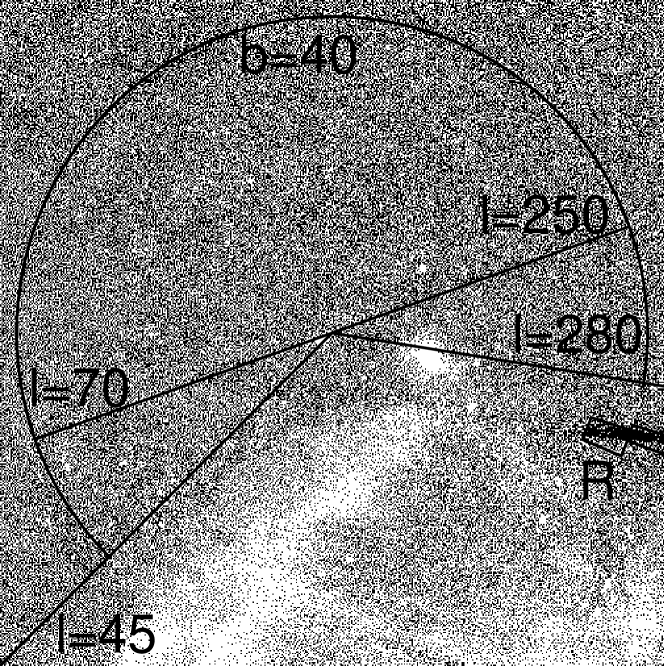
Figure 1: Section of the RASS centered on the North Galactic Pole in an equal area projection. The whole map covers $3.19$ Sr. The areas defined in Table 1 used in the computations are marked. The small region marked ‘R’ has been removed from the data because of insufficient exposure time.

The data from the north galactic hemisphere are used. The XRB flux is binned into $12^{\prime}\times 12^{\prime}$ pixels composing an array of $512\times 512$ elements. An equal-area polar projection centered on the North Galactic Pole has been applied to record the data. Within this area a small patch of sky marked ‘R’ in Fig. 1 has not been covered by the RASS. A large portion of the north galactic hemisphere is dominated by the hot plasma emission in our Galaxy (Snowden et al. 1995). Most of this local signal is concentrated at galactic longitudes between $260^{\circ}$ and $50^{\circ}$. The remaining area is visually free from the foreground galactic signal, but some local contribution is also present (Soltan et al. 1996, 1999). To investigate effects of the galactic contamination on our determinations of the power spectrum, computations have been performed using various subsets of the available data.

The regions investigated in detail in the present analysis are defined in Table 1. The total area (‘A’ in Table  1) is highly non-homogeneous because of the galactic component. The spherical harmonic transform for this area has been computed mainly as a check of our algorithm (see below). Area ‘B’ is the largest fragment of the northern celestial hemisphere apparently free from strong galactic emission. However, the border regions of this area are close to prominent emission regions. Area ‘B’ extends also to low galactic latitudes ($b<20^{\circ}$ at the ”corners” of the RASS map) and effects of the galactic obscuration are likely to be present. Thus, one could expect some interference of galactic and extragalactic signals. Area ‘C’ is restricted to the galactic latitudes $b>40^{\circ}$. The smallest area , ‘D’, has been extensively analyzed by Soltan et al. (1996, 1999). The power spectrum obtained for this region should correspond to the autocorrelation function obtained in those papers. To see the effects on our results of the brightest sources, some computations were performed without two conspicuous clusters: Coma and Abell 1367.

Table 1
Sample	$l_{min}$	$l_{max}$	$b_{min}$	$\Omega$[Sr]
A	$0^{\circ}$	$360^{\circ}$	$12^{\circ}-37^{\circ\dagger}$	$3.18^{\ddagger}$
B	$45^{\circ}$	$280^{\circ}$	$12^{\circ}-37^{\circ\dagger}$	$2.04$
C	$45^{\circ}$	$280^{\circ}$	$40^{\circ}$	$1.43$
D	$70^{\circ}$	$250^{\circ}$	$40^{\circ}$	$1.12$

^† Minimum galactic latitude varies with the galactic longitude (see Fig. 1).
^‡ After removal of region ‘R’.

3 The power spectrum

Although the definitions and basic relationships for spherical harmonics are outlined in a number of astrophysical publications, we describe below in some detail the standard formulae and all the essential steps of our analysis in order to present it in a complete and coherent way. Where possible, we followed the notation used by Peebles (1973) and Hauser & Peebles (1973).

3.1 Sky coverage

Spherical harmonic functions constitute a set of orthogonal functions on the sphere. Astrophysical data rarely cover a full solid angle of $4\pi$. In the present investigation the useful data are also available for a limited region of the sky only. Incomplete sky coverage destroys the orthogonality of the spherical harmonic functions. Consequently, the power spectrum coefficients are correlated (Hauser & Peebles 1973). There are basically two ways to take this effect into account. One can either construct a new set of functions which are orthogonal in the defined area of the sphere (e.g. Górski 1994, Tegmark 1996), or fill the area where the observational material is missing with synthetic data (see below). Both methods have their advantages as well as drawbacks. In the present paper we use the latter approach for two reasons. Firstly, we perform calculations using data selected in several regions of the sky. Different windows imply different sets of orthogonal functions, which makes comparison of the results ambiguous. Secondly, we are interested in XRB fluctuations at angular scales significantly smaller than the size of the area covered by the data. A section of the harmonic power spectrum corresponding to these small scales is adequately determined using the available RASS data.

3.2 Spherical harmonics - the formulae

The distribution of the XRB flux on the celestial sphere, $\rho(\theta,\phi)$, is represented as an infinite sum of spherical harmonics $Y_{l}^{m}$:

$$\rho(\theta,\phi)=\sum_{l=0}^{\infty}\,\sum_{m=-l}^{l}\;a_{l}^{m}\,Y_{l}^{m}(\theta,\phi),$$ (1)

where the coefficients $a_{l}^{m}$ are the spherical harmonic transform:

$$a_{l}^{m}=\int_{4\pi}\,\rho(\theta,\phi)\>Y_{l}^{m\ast}(\theta,\phi)\>d\Omega\,.$$ (2)

The RASS covers practically the whole celestial sphere, but only relatively small regions of the sky contain the data dominated by the extragalactic signal; the remaining areas are heavily contaminated by local effects. As a result of this, we are forced to carry out the power spectrum analysis using the data from a fraction of the sky. To assess the effects of incomplete sky coverage we introduce, following Peebles (1973), the window function, $W(\theta,\phi)$, which describes the area used in the analysis:

$$W(\theta,\phi)=\cases{1,&\hbox{inside the accepted region,}\cr 0,&\hbox{outside the accepted region.}}$$ (3)

Using the window function we define for the whole celestial sphere a model distribution of the XRB:

$$\tilde{\rho}(\theta,\phi)=W(\theta,\phi)\,\rho(\theta,\phi)+[1-W(\theta,\phi)]\,\langle\rho\rangle\,,$$ (4)

where $\langle\rho\rangle$ is the mean background flux averaged over the accepted area. Thus, within the window area the model distribution is identical to the actual one, while outside the window it is constant and equal to the average signal computed using the data just from the accepted region. The model distribution covers the whole sphere, but the cosmic information is limited to the window area.

The spherical harmonic transform of $\tilde{\rho}$,

$$\tilde{a}_{l}^{m}=\int_{4\pi}\,\tilde{\rho}\>Y_{l}^{m\ast}\,d\Omega\,,$$ (5)

and $\tilde{\rho}$ is related to the $\tilde{a}$’s by a formula analogous to Eq. (1). Using Eq. (4) we get:

$$\tilde{a}_{l}^{m}=\cases{\int_{\Omega}\,\rho\>Y_{l}^{m\ast}\>d\Omega-\langle\rho\rangle\,\int_{\Omega}\,Y_{l}^{m\ast}\,d\Omega,&\hbox{for $l\neq 0$,}\cr\sqrt{4\pi}\,\langle\rho\rangle,&\hbox{for $l=0$,}}$$ (6)

where the integrals extend over the solid angle, $\Omega$, of the accepted area. The zero degree term, $\tilde{a}_{0}^{0}$, represents the average signal in the data and does not depend on the window function. One should note that coefficients $\tilde{a}_{l}^{m}$, although calculated using the cosmic data from the fraction of the sky, represent a mathematically well defined spherical harmonic transform. In particular, the expected values of all the $l\neq 0$ coefficients $\tilde{a}_{l}^{m}$ are equal to 0. Eq. (6) implies that

$$\left\langle\int_{\Omega}\,\rho\>Y_{l}^{m\ast}\,d\Omega\right\rangle=\langle\rho\rangle\int_{\Omega}\,Y_{l}^{m\ast}\,d\Omega\,,$$ (7)

where $\langle...\rangle$ enclosing the integral denote the expectation value. Eq. (7) shows that the ‘spherical harmonic transform’ coefficients calculated from a fraction of the sphere deviate systematically from zero (see Peebles (1973) for a detailed discussion).

One should expect that at angular scales substantially smaller than the characteristic size of the window, the fluctuations of the XRB are adequately described by $\tilde{a}_{l}^{m}$. In order to find a relationship between $\tilde{a}_{l}^{m}$ and ${a}_{l}^{m}$, we use the angular autocorrelation function (ACF), $w(\theta)$:

$$w(\theta)={{\left\langle\rho(\omega_{1})\,\rho(\omega_{2})\right\rangle}_{\mid{4\pi}}\over\langle\rho\rangle^{2}}-1\,,$$ (8)

where $\omega_{i}=(\theta_{i},\phi_{i})$ for $i=1,2$ denote points in the celestial sphere separated by the angle $\theta$ and the average values $\langle...\rangle$ are calculated for the whole sphere. Using Eq. (B2) of Peebles (1973) and Eq. (1) one obtains the relationship between the average flux correlation and the spherical harmonic transform:

$${\left\langle\rho(\omega_{1})\,\rho(\omega_{2})\right\rangle}_{\mid{4\pi}}=\sum_{l=0}\;\sum_{m=-l}^{l}\mid\!a_{l}^{m}\!\mid^{2}\,{P_{l}(\cos\theta)\over 4\pi}$$ (9)

$$\phantom{{\left\langle\rho(\omega_{1})\,\rho(\omega_{2})\right\rangle}_{\mid{4\pi}}}=\langle\rho\rangle^{2}+\sum_{l=1}{2l+1\over 4\pi}Z_{l}\,P_{l}(\cos\theta)\,,$$

where

$$Z_{l}={1\over 2l+1}\,\sum_{m=-l}^{l}\mid\!a_{l}^{m}\!\mid^{2}$$ (10)

is the power spectrum for the distribution on the sphere, and $P_{l}$ is a Legendre function of degree $l$. In an analogous way we define the power spectrum of the model distribution $\tilde{\rho}$:

$$\tilde{Z}_{l}={1\over 2l+1}\,\sum_{m=-l}^{l}\mid\!\tilde{a}_{l}^{m}\!\mid^{2}\,.$$ (11)

Eqs. 8, 9 and 10 give

$$w(\theta)={1\over\langle\rho\rangle^{2}}\;\sum_{l=1}{2l+1\over 4\pi}\,Z_{l}\,P_{l}(\cos\theta)\,,$$ (12)

and an analogous relationship between $\tilde{w}$ and $\tilde{Z}_{l}$. If we now limit our analysis to separation angles small in comparison to the size of the area of solid angle $\Omega$, we may express the average product of the model flux $\langle\tilde{\rho}(\omega_{1})\,\tilde{\rho}(\omega_{2})\rangle_{\mid 4\pi}$ as the sum of two components (using Eq. (4)):

$$\langle\tilde{\rho}(\omega_{1})\,\tilde{\rho}(\omega_{2})\rangle_{\mid 4\pi}\approx{\Omega\over 4\pi}\,\langle\rho(\omega_{1})\,\rho(\omega_{2})\rangle_{\mid\Omega}+{4\pi-\Omega\over 4\pi}\,\langle\rho\rangle^{2}\,,$$ (13)

where on the left hand side the averaging is over the whole sphere, while on the right hand side it is done over a solid angle of $\Omega$. One can transform this equation into:

$$\tilde{w}(\theta)={\Omega\over 4\pi}\,w_{\Omega}(\theta)\,,$$ (14)

where $w_{\Omega}$ is the autocorrelation function calculated using the data within the solid angle $\Omega$. As long as the cosmic signal contained within the window is a fair sample of the entire XRB, $w_{\Omega}(\theta)=w(\theta)$. Thus, scaling of the ACFs (Eq. (14)) together with Eqs. (10) and (11) gives

$$Z_{l}={4\pi\over\Omega}\,{1\over 2l+1}\,\sum_{m=-l}^{l}\mid\!\tilde{a}_{l}^{m}\!\mid^{2}\,,$$ (15)

in agreement with Eqs. (53) and (54) by Peebles (1973). Eq. (15) shows that the high $l$ part of the power spectrum (for the whole sphere) is directly proportional to the power spectrum based on the data from the fraction of the sphere if these data are representative for the whole sphere (fair sample assumption).

3.3 Spherical harmonics - computations

Figure 2: Count rate distribution in the R6 energy band of the RASS in $12^{\prime}$ pixels along galactic longitude $l=0$. The data in this region are heavily contaminated by galactic emission which causes large-scale variations in the count rate. The curves show the synthesized distribution for $l_{\rm max}=450$, 900, and 1800.

Figure 3: Same as Fig. 2 for galactic longitude $l=90^{\circ}$. Most of the signal is of extragalactic origin. Because of the negligible galactic contribution, the average count rate is lower than in Fig. 2. Note the good fit for $l_{\ rmmax}=1800$ (bottom panel).

The large survey area combined with a relatively high angular resolution of the RASS allows us to calculate the power spectrum over a wide range of the spherical harmonic degree $l$. Fluctuations of the XRB on the scale $\theta$ will produce a signal in the power spectrum at $l\sim\pi/\theta$. Since the pixel size of the RASS is $12^{\prime}$, our algorithm should be effective up to $l\sim 900$. Fortunately this requirement could be satisfied with the present day computers without major problems.

The spherical harmonic function is defined in a standard way by:

$$Y_{l}^{m}(\theta,\phi)=c_{l}^{m}\,P_{l}^{m}(\cos\theta)\,e^{im\phi}\,,$$ (16)

$$c_{l}^{m}=\left[{2l+1\over 4\pi}\,{(l-m)!\over(l+m)!}\right]^{1/2}\,,$$

$$P_{l}^{-m}(x)=(-1)^{m}\,{(l-m)!\over(l+m)!}\,P_{l}^{m}(x)\,.$$

where $P_{l}^{m}$ are the associated Legendre polynomials. For positive m these are defined by the formula:

$$P_{l}^{m}(x)=(-1)^{m}\,(1-x^{2})^{m/2}\,{d^{m}\over dx^{m}}P_{l}(x)\,.$$ (17)

Using the above relations it can be seen that

$$Y_{l}^{-m}(\theta,\phi)=(-1)^{m}\,Y_{l}^{m\ast}(\theta,\phi)\,.$$ (18)

In the actual computations it is convenient to use recursive formulae rather than Eqs. (16) and (17) directly. We use the relations given by Brauthwaite (1973) as quoted by Hauser & Peebles (1973). To verify the accuracy of our computations and demonstrate the effects of the maximum harmonic order on the resolution and quality of the fits, we synthesized the model distribution using Eq. (1) and the spherical harmonic transform coefficients $\tilde{a}_{l}^{m}$. Because of the finite number of spherical harmonics used in the calculations the synthesized map does not reproduce exactly the original RASS data.

In Fig. 2 we show a sample distribution of count rates in 146 pixels along the line of galactic longitude $\ell=0$ between galactic latitudes $50^{\circ}$ and $80^{\circ}$ . The three panels show the synthesized distributions for three values of the maximum spherical harmonic degree used in the calculations, $l_{\rm max}=450$, $900$, and $1800$. The spherical harmonic transform $\tilde{a}_{l}^{m}$ was calculated for the total area of roughly $3.2$ sr shown in Fig. 1. In the top panel with $l_{\rm max}=450$ the synthesized distribution follows the large scale features of the real distribution. The minimum angular scale ‘resolved’ in this model corresponds roughly to 2 RASS pixels. The fit to the real signal looks bad because the model locally represents the signal averaged over $\sim 4$ pixels and the scan in Fig. 2 has the width of a single pixel. The fit is substantially improved in the middle panel where $l_{\rm max}=900$ and still further in the lower panel for $l_{\rm max}=1800$. It is evident that to reproduce details of the XRB distribution binned into $12^{\prime}\times 12^{\prime}$ pixels the harmonic decomposition has to reach the degree of $l_{\rm max}\approx 900$. The model with $l_{\rm max}=1800$ reproduces the features of the cosmic signal very accurately. We treat this as a verification of our computational algorithm. In Fig. 3 the section of the RASS for galactic longitude $90^{\circ}$ is shown. Here the contamination by the galactic plasma emission is small and the signal is dominated by the extragalactic component. The conspicuous large-scale trends are absent in this region and the fluctuations are dominated by point-like sources. Similar to Fig. 2 the goodness of the fit improves substantially with increasing $l_{\rm max}$. In particular, the fits for $l_{\rm max}\ga 900$ adequately reproduce the peaks associated with bright sources.

3.4 Effects of pixelization of the data

The power spectrum at high $l$ is affected by the pixelization of the XRB data. The XRB fluctuations at scales smaller than the pixel size are smoothed over the pixel area modifying the flux correlation at this angular scale and removing the variations at smaller scales. We assess these effects as follows.

3.4.1 Fluctuations below the pixel size

Figure 4: A - Power spectrum of all data (Sample A); M - model which shows the contribution to the overall spectrum by fluctuations at scales below the pixel size.

The count rate fluctuations recorded in the $12^{\prime}$ RASS pixels result from the cosmic variations and the photon noise. Cosmic variations are produced mainly by discrete sources and should be distributed uniformly (apart from the source clustering) at high galactic latitudes. On the other hand, the amplitude of the fluctuations generated by the photon statistics depends on the exposure time and varies over the survey area. In principle, this property should help to distinguish between these two sources of fluctuations. We plan to analyze this effect in the future paper. Due to the presence of extended X-ray sources and source clustering, the cosmic signal binned in pixels is correlated, while the fluctuations generated by the photon noise are uncorrelated.

Uncorrelated fluctuations generate the flat power spectrum over all $l\la 900$. To assess the contribution to the power spectrum by fluctuations at scales below the pixel size, we calculate the model spectrum assuming that the count rates in pixels are uncorrelated. We use a formula analogous to Eq. (22) of Peebles (1973):

$$\langle\mid\!a_{l}^{m}\!\mid^{2}\rangle=2\pi\langle\rho\rangle^{2}\int_{-1}^{+1}w(\theta)\,P_{l}(\cos\theta)\,d\cos\theta\,,$$ (19)

which is obtained from Eq. (2) above and Eq. (B2) of Peebles (1973). It is straightforward to calculate the exact shape of the autocorrelation function assuming a ‘flat’ X-ray signal within each pixel and no correlation between pixels. Such a synthetic autocorrelation function depends only on the second moment of the count rates in the pixels and on the pixel size (and shape); this model autocorrelation function is equal to zero for separations which are not contained within a single pixel. The solid curve in Fig. 4 shows the power spectrum $Z_{l}$ calculated for the total area (Sample A of Table 1) and the dashed curve represents the model power spectrum, assuming that the fluctuations in $12^{\prime}$ pixels are uncorrelated. The observed power spectrum is fitted well by the model for $l\ga 700$ and has a systematically larger amplitude for smaller $l$. This demonstrates that the cosmic signal is strongly correlated over a wide range of separations. Additionally, good agreement in the high-$l$ range, where potentially numerical problems could develop, indicates that our algorithm is accurate over the entire range of $l$.

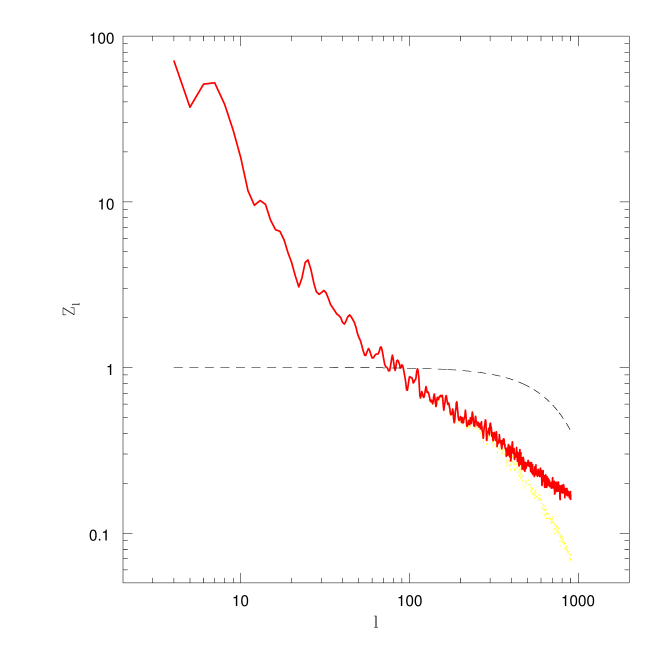
Figure 5: The raw power spectrum of all data. Sample A: dotted curve; the corrected spectrum: solid curve; the correction for the finite pixel size: dashed curve.

3.4.2 Corrections for moderate harmonic scales

The dashed curve in Fig. 4 shows that binning the data into $12^{\prime}$ pixels reduces the amplitude of the power spectrum also at degrees below $l=900$. To account for this effect we have calculated the distortion of the power spectrum generated by the binning. The model power spectrum $Z_{l}=1$ was used as input data. This flat spectrum represents a random distribution of point sources. Due to the binning of the input flux, the resulting power spectrum has a shape analogous to the model marked ‘M’ in Fig. 4. The ratio of the modified power spectrum to the input model is shown in Fig. 5 by a dashed line. To correct for this effect one should normalize the raw RASS spectra by this curve. In Fig. 5 the dotted curve represents the raw spectrum of the XRB in area ‘A’, and the solid curve shows the corrected spectrum. The spurious curvature of the spectrum caused by the data binning is removed. This procedure is effective up to a harmonic degree of $l\approx 900$ and is applied to all subsequent power spectra computations.

4 Results

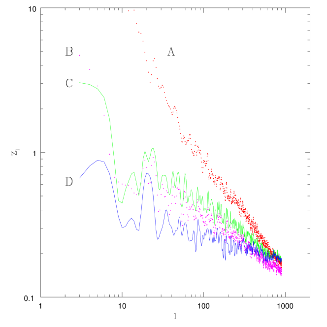
Figure 6: Power spectra of the XRB in the R6 band. Labels ‘A’, ‘B’, ‘C’ and ‘D’ denote the RASS regions defined in Table 1.

In Fig. 6 the power spectra of the R6 band are shown for four regions of the RASS defined in Table 1.

The spherical transform at low degrees is corrupted by the window function. The maximum angular scale effectively accessible to the analysis is several times smaller than the size of the area used in the computations. The strong oscillations of $Z_{l}$ for areas ‘B’ – ‘D’ visible in Fig. 6 indicate that the power spectrum estimates of any individual degree $l$ are subject to large uncertainties at low $l$ values. Assuming that the ‘true’ shape of the power spectrum is more regular than that in Fig. 6, one can try to fit a smooth function. This would extend our $Z_{l}$ estimates down to $l\approx 10$.

Apart from small $l$ variations none of the spectra exhibits any distinct features in the entire range of degrees. The lack of significant spectral structures is also apparent in Fig. 9. The RASS data have been accumulated in the scanning mode of the satellite operation. Thus the raw data consist of a large number of $\sim 2^{\circ}$ wide strips along great circles of constant ecliptic longitudes. In a laborious procedure (Snowden et al. 1995 and references therein) these raw counts have been reduced to create a homogeneous map of the XRB flux. Despite a great effort to remove all the artifacts produced by the data accumulation technique, one should be concerned that not all the instrumental effects have been removed from the final maps. Our power spectra do not show visible features at degrees corresponding to an angular scale of $2^{\circ}$, which indicates that the XRB maps are free from noticeable effects generated by the scanning mode.

The conspicuous difference of the power spectrum at low degree $l$ between area ‘A’ and the remaining areas results from strong contamination by galactic emission between galactic longitudes $280^{\circ}$ and $45^{\circ}$. One should also note that the power spectrum amplitude for area ‘D’ is systematically smaller than for areas ‘B’ and ‘C’. This difference indicates that the contribution of the hot galactic plasma to the background is not confined to the region between $280^{\circ}$ and $45^{\circ}$ but extends further away. It is important that, apart from differences at small $l$, all power spectra converge at high $l$, indicating that fluctuations at the smallest scales are dominated by the extragalactic component. Although the contribution of the hot plasma to the spectrum at larger scales is substantially reduced in area ‘D’ in comparison with the remaining areas, it is still possible that some signal is generated locally. To investigate this problem, we now concentrate on the analysis of region ‘D’.

4.1 Error estimates

Our estimates of the power spectrum are subject to two sources of errors. Limited counting statistics and instrumental background subtraction produce uncertainties in the distributions of the XRB flux in the RASS data. Information on the expected rms count rate uncertainty for each pixel has been obtained during the RASS production process and is stored in a separate array. We used these data to generate 24 simulated RASS maps. For each simulation the count rates in all pixels have been randomized using a Gaussian distribution with an average equal to the real count rate and a variance taken from the uncertainty array. The power spectra of all the simulations have been computed. The rms scatter between these simulated functions is used as an estimate of the $1\sigma$ uncertainty of the power spectrum of the real data. The corresponding error bars are shown in Fig. 7a for one of the spectra of area ‘D’.

A second source of uncertainty is related to the cosmic variance. To account for this effect, we have divided area ‘D’ into 6 sections and computed the power spectra for each region separately. The scatter between the spectra of the 6 regions is used to estimate the uncertainty of the spectrum based on the entire area ‘D’. The resultant error bars are shown in Fig. 7b. Since the average exposure times in the RASS are rather short, the uncertainties in the count rate for individual pixels are relatively high. Nevertheless, one should note that the uncertainties introduced by cosmic variance are larger than the errors generated by poor counting statistics.

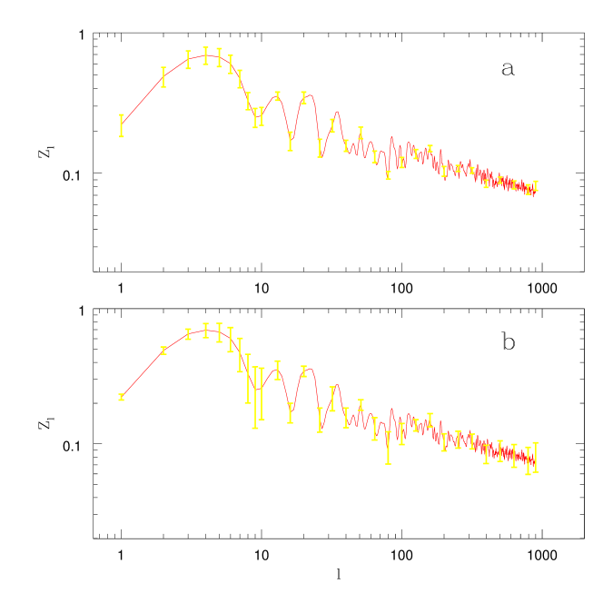
Figure 7: Uncertainties of the power spectrum estimates produced by photon counting statistics (a) and cosmic variance (b). Area ‘D’ is used. The error bars represent $1\sigma$ uncertainties. For clarity, the error bars are plotted for selected degree $l$.

4.2 The power spectrum of the R6 band

Figure 8: The cumulative distribution of the count rates in the pixels in area ‘D’ in the R6 band. The solid curve gives the number of $12^{\prime}\times 12^{\prime}$ pixels with a count rate above the specified value; the dashed curve gives the complementary distribution. Linear and log scales are used for low and high count rate sections of the distribution. The vertical dotted line (which splits the plot) marks the median of the distribution. Arrows indicate the cutoffs used in the calculations (see text).

The power spectra shown in Fig. 6 are calculated using all the XRB flux in the specified area including strong sources. Many of these sources produce count rates which exceed the average count rate per pixel by a factor of ten or more. In Fig. 8 we have plotted the cumulative distribution of the count rates in the R6 band for area ‘D’. The distribution has a long high count rate tail extending to above $28\cdot 10^{3}$, while the average of the distribution is equal to $\sim 80$. The highest signal, viz. 28175, in the R6 band is generated by a source associated with the Seyfert galaxy IC 3599 (Komossa & Bade 1999). In $0.1$ % of pixels the count rate exceeds $904$ and in $1.0$ % it exceeds $256$. Such peaks generate a signal in the power spectrum over all harmonic degrees. To see what impact these strong peaks have on the resulting power spectrum we have calculated the spectra using the data without the brightest sources. This was achieved by modifying the window function (Eq. (3)) to exclude pixels with count rates above the assumed threshold. The effects of the high count rate tail on the power spectra are shown in Fig. 9.

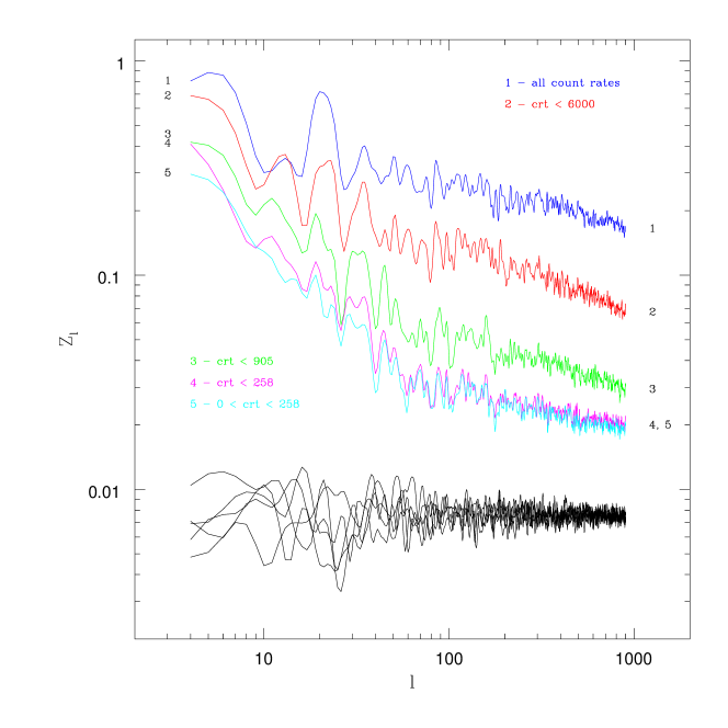
Figure 9: The power spectra in area ‘D’ with different thresholds imposed on the count rates: 1: all data (same as in Fig. 6); 2: the pixel with the highest count rate has been removed; 3: the pixels with the top $0.1$ % count rates have been removed; 4: the pixels with the top $1.0$ % count rates have been removed; 5; the pixels with the top $1.0$ % count rates and with negative count rates have been removed; the curves in the lower part represent five simulations (see text).

Since the narrow peaks in the distribution produce a signal in the harmonic power spectrum over the entire range of degrees $l$, the removal of the brightest sources from the area reduces the amplitude of the power spectrum over a wide range of degrees. As a result of the subtraction of the peaks the shape of the spectrum changes significantly. For the whole data (Fig. 9, spectrum No 1) it is roughly a power law for $l<900$, while spectrum No 4 which represents the data without the brightest sources is well approximated by a broken power law with steep slope at degrees below $\sim 60$ and distinctly flatter slope at larger $l$.

The effects of uncorrelated fluctuations are shown in the lower part of Fig. 9. We have plotted there spectra of five simulated distributions. In the simulations the count rates in the pixels were completely uncorrelated and the distribution of the count rates in the pixels was Gaussian with a mean value of $75$ and a dispersion of $25$. As expected, the simulated spectra are flat. The scatter between the simulations reflecting the stochastic nature of the problem indicates the level of uncertainties involved in the spectrum estimates.

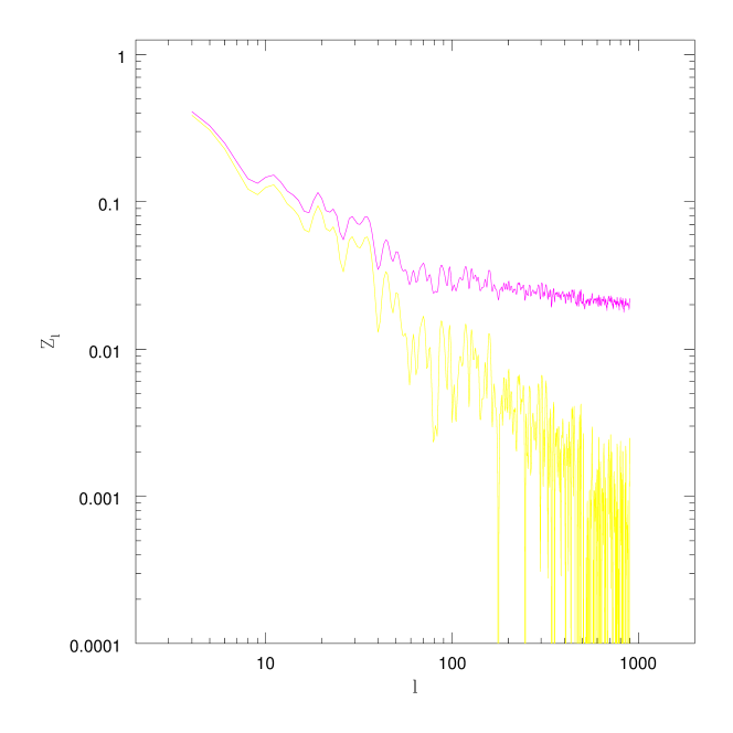
Figure 10: An example of the decomposition of the observed spectrum; upper curve: the power spectrum of the data in area ‘D’ after the removal of 1 % pixels with the highest count rates (same as spectrum No 4 in Fig. 9); lower curve: the residual spectrum obtained from the upper curve by subtraction of the flat spectrum representing randomly distributed sources contributing most to the high $l$ part of the total spectrum (see text).

Before we investigate this question in detail, it is worth noting that the pixels with the lowest count rates do not affect significantly the estimates of the power spectrum. The low-count-rate part of the distribution is sensitive to errors in the instrumental background subtraction. As a result of inaccuracies in this procedure, the XRB signal formally assigned to more than 1000 pixels is negative. However, negative count rate pixels do not create a long tail in the pixel distribution and do not influence the overall power spectrum. This is shown in Fig. 9 by spectra No 4 and 5. In both cases an upper count rate threshold of 256 was used, and in spectrum No 5 all pixels with negative count rates have also been removed.

A variety of sources contributing to the XRB produce its complex structure. Sources which are spatially unrelated (e.g. nearby galaxies and distant AGNs or extragalactic sources and the local Galactic emission) create patterns on the celestial sphere with characteristic and mutually independent statistical properties. Thus, the power spectrum of the total XRB signal is a sum of several distinct components corresponding to separate XRB constituents. The present data do not constrain strongly amplitudes of individual potential components of the measured spectrum. To illustrate this we consider spectrum No 4 shown in Fig. 9. The flat high degree part of this spectrum indicates that a substantial fraction of the signal in this range of $l$ is produced by small scale fluctuations which are generated mainly by point-like sources. The distribution of these sources is not constrained. They may be distributed nonuniformly and contribute also to the large scale fluctuations described by the low $l$ section of the spectrum or they may be distributed randomly so that the entire signal at small $l$ is due to the other sources contributing to the XRB. In the framework of the latter model, there are two separate populations contributing to the XRB. The spectra of both components have been estimated in the following way. Using the procedure described in Sect. 3.4.1 we calculated the model spectrum assuming that the count rates in the pixels are completely uncorrelated. This spectrum was then subtracted from the No 4 spectrum; the residual spectrum is shown in Fig. 10. The decomposition of the observed spectrum represents a model in which strong sources produce local fluctuations, while most of the signal at large angular scales is generated by a smooth distribution. Its contribution to the local fluctuations is negligible.

4.3 Power spectra vs. energy

Because the RASS data useful for the extragalactic analysis cover a narrow range of energies and the ROSAT  energy bands overlap substantially, the power spectra of R5, R6 and R7 share many common features. Nevertheless they exhibit some differences which can be ascribed to a slightly different content of the XRB at these energies. In Figs. 11, 12 and 13 the power spectra of area ‘D’ of the RASS are shown in three energy bands. The spectra plotted in Fig. 11 are calculated after the removal of the pixel with the highest count rate in the field (produced by a Seyfert galaxy, IC 3599); in Figs. 12 and 13 the pixels of the top $0.1$ % and $1.0$ % count rates were removed.

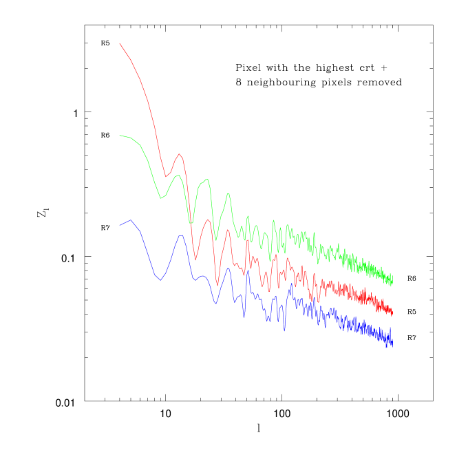
Figure 11: The harmonic power spectra of the RASS energy bands R5, R6 and R7; area ‘D’ is used. One pixel (the same in all the bands) with the highest count rate is removed from the data.

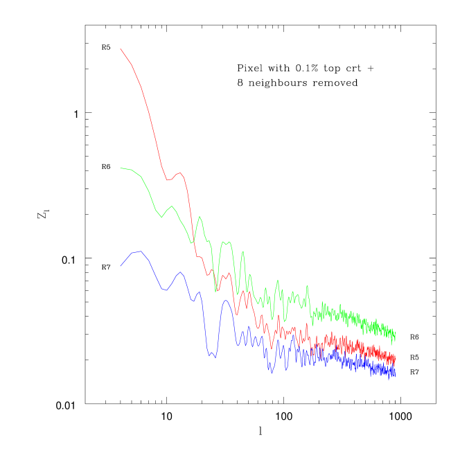
Figure 12: Same as Fig. 11; the pixels with the top $0.1$ % count rates are removed.

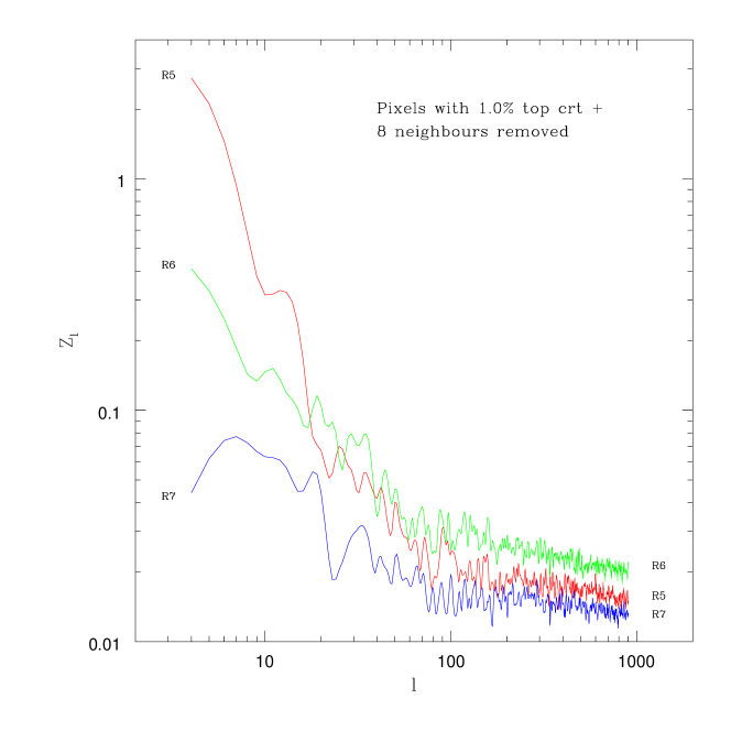
Figure 13: Same as Fig. 12; the pixels with the top $1.0$ % count rates are removed.

In each subsample the spectra of all three bands, R5, R6 and R7 exhibit a similar slope at degrees above $l\sim 200-300$. Also the normalization of all spectra at high $l$ end is consistent with the conjecture that the amplitudes of the fluctuations at small angular scales are proportional to the average signal in each energy band. This implies that small-scale fluctuations have the same “colors” as the average XRB.

The similarity of the R6 and R7 spectra continues to small degrees $l$ and both these spectra differ significantly from the spectrum of the softest band R5. The latter spectrum exhibits a sharp increase below $l\sim 20$ in Figs. 11 and $l\sim 100$ in Figs. 12 and 13. This is a result of the contamination of the R5 band by soft photons, which evidently exhibit large-scale non-uniformities. The spectra of subsamples devoid of the strongest sources reveal a change of slope at quite small angular scales of a few degrees. Evidently, the excess fluctuations of the soft XRB over the harder component represent a separate XRB component whose origin deserves careful examination.

4.4 The autocorrelation function

The power spectrum may be used to calculate the autocorrelation function (ACF). In the previous sections the relationship between those two statistics has been used to elucidate the effects of the data binning. Here we employ this relationship (Eq. (12)) to calculate the ACF for the whole separation range and to compare it with the ACF determinations given by Soltan et al. (1996, 1999). The relationship between ACF and harmonic power spectrum is discussed in the Appendix.

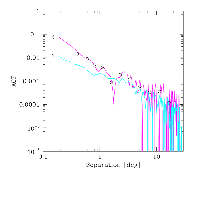
Figure 14: The autocorrelations functions of area ‘D’. Labels ‘2’ and ‘4’ denote the ACFs computed from the power spectra in Fig. 9 marked ‘2’ and ‘4’, respectively. The ACF calculated directly from the data in subsample No ‘2’ is shown by open circles.

The ACF computed using two power spectra, No 2 and 4 in Fig. 9 is shown in Fig. 14. For comparison, open circles show the ACF computed directly from the RASS data using the same subsample as for the curve labelled ‘2’. It is clearly visible that the removal of the strongest sources from the area reduces significantly the ACF at separations below $\sim 1^{\circ}$. This implies that these sources are not distributed randomly. The residual ACF signal shows that the XRB devoid of the brightest sources still exhibits fluctuations. But the substantial decrease of the ACF amplitude after the removal of $1$ % of pixels indicates that the origin of the XRB fluctuations requires further studies.

5 Prospects for the future

Deciphering the XRB fluctuations plays a crucial role in the investigation of various components of the background. In the present work we have calculated the harmonic power spectrum of several subsamples of the RASS. The data have been selected according to various criteria such as the energy band, amount of the galactic contamination and presence of strong sources. The corresponding power spectra reveal the effects of the different selection criteria. This gives good prospects to use the spectra to investigate models of the XRB.

Such models should specify the relative contributions of various classes of discrete sources contributing to the XRB as well as the amount of the thermal emission generated by hot gas which according to Cen & Ostriker (1999) is accumulating in the gravitational potential wells of galaxies and galaxy agglomerations. Since the temperature of the gas is relatively low one expects that the energy spectra of discrete sources and of thermal emission are distinctly different. Also a smooth gas distribution would not produce sharp peaks in the XRB. These factors could help to differentiate between the two XRB components by means of the power spectrum and ACF analysis. Such investigation should also utilize the small scale XRB fluctuation measurements based on the ROSAT  pointings.

APPENDIX
The ACF amplitude difference at small separations between ACFs in Fig. 14 is in agreement with the expected correspondence that the larger amplitude of the spectrum at high degree $l$ generates the stronger signal of the ACF at small separations. However, the relationship defined by Eq. (12) does not yield a plain dependence of the ACF slope on the slope of the power spectrum $Z_{l}$. Generally the power law shape of the spectrum does not produce the power law shape of the ACF. However, for the special case of $Z_{l}\sim l^{-1}$ Eq. (12) generates an ACF which is well approximated by a power law with a slope of $-1$. The exact solution differs from the power law $w(\theta)\sim 1/\theta$ by less than $5$ % for separations $\theta<18.\!\!^{\circ}5$.

One should note that distinctly different harmonic power spectra could produce similar ACFs. For instance, the ACFs calculated using spectra plotted in Fig. 10 are identical for separations above $\sim 0.\!\!^{\circ}3$ despite large and systematic differences in the input spectra. This is because the flux correlations between pixels are the same in both cases. The lower spectrum has been obtained from the upper one by subtracting the flat spectrum which represents random (uncorrelated) fluctuations. Thus, both spectra describe distributions with the same correlation properties.

ACKNOWLEDGEMENTS. The ROSAT  project has been supported by the German Bundesministerium für Bildung und Forschung/Deutsches Zentrum für Luft- und Raumfahrt (BMBF/DLR) and by the Max-Planck-Gesellschaft (MPG). This work has been partially supported by the Polish KBN grant 5 P03D 022 20.

References

- Barcons (1998) Barcons X., Fabian A. C., Carrera F. J., 1998, MNRAS 293, 60
- Brauthwaite (1973) Brauthwaite, W., 1973, Computer Physics Communications, 5, 390
- Cen & Ostriker (1999) Cen, R., & Ostriker, J. P., 1999, ApJ 514, 1
- Giacconi et al. (1962) Giacconi R., Gursky H., Paolini F. R., Rossi B. B., 1962, Phys. Rev. Letters, 9, 439
- Giacconi et al. (1979) Giacconi, R., Bechtold, J., Branduardi, G., et al., 1979, ApJ 234, L1
- Górski (1994) Górski, K. M., et al., 1994 ApJL 430, L85
- Hasinger (1992) Hasinger, G., 1992, in The X-ray Background, eds. X. Barcons, A. C. Fabian, (Cambridge U. Press: Cambridge), 299
- Hasinger (1998) Hasinger G., Burg, R., Giacconi, et al. 1998, A&A 329,482
- Hauser & Peebles (1973) Hauser, M. G. & Peebles, P. J. E., 1973 ApJ 185, 757
- Kneissl et al. (1997) Kneissl, R., Egger, R., Hasinger, G., Soltan, A., & Trümper, J., 1996, A&A 320, 685
- Komossa & Bade (1999) Komossa, S., & Bade, N., 1999, A&A 343, 775
- Krautter (1999) Krautter, F. J., Zickgraf., et al. 1999, A&A 350, 743
- Lahav et al. (1993) Lahav, O., Fabian, A. C., Barcons, X., et al., 1993, Nature 365, 693
- Miyaji et al. (1994) Miyaji, T., Lahav, O., Jahoda, K., & Boldt, E., ApJ 434, 424
- Phillips et al. (2000) Phillips, L. A., Ostriker, J. P., & Cen, R., 2000, astro-ph/0011348
- Plucinsky et al. (1993) Plucinsky P. P., Snowden S.L., Briel U. G., Hasinger G., Pfefferman E., 1993, ApJ 418, 519
- Peebles (1973) Peebles, P. J. E., 1973 ApJ 185, 413
- Roche et al. (1995) Roche, N., Shanks, T., Georgantopoulos, I., Stewart, G. C., Boyle, B. J., & Griffiths, R. E., 1995, MNRAS 273, L15
- Setti et al (1989) Setti G., Woltjer L., 1989 A&A 224 L21
- Scharf et al. (2000) Scharf, C. A., Jahoda, K., Treyer, M., Lahav, O., Boldt, E., Piran, T., 2000 ApJ 544, 49
- Snowden et al. (1997) Snowden S.L., Egger R., Freyberg M.J., et al. 1997 ApJ 485, 125
- Snowden et al. (1995) Snowden S.L., Freyberg, M. J., Plucinsky, P. P., et al. 1995 ApJ 454, 643
- Snowden et al. (1994) Snowden S.L., McCammon D., Burrows D., Mendenhall J.A., 1994, ApJ 424, 714
- Snowden & Schmitt (1990) Snowden, S. L., & Schmitt, J. H. M. M., Ap&SS 171, 207
- Soltan et al. (1996, 1999) Sołtan A.M., Freyberg M., Hasinger G., Miyaji T., Treyer M., Trümper J. 1999, A&A, 349, 354
- Soltan et al. (1996) Sołtan A. M., Hasinger G., Egger R., Snowden S., Trümper J., 1996, A&A 305, 17
- Soltan et al. (1997) Sołtan A. M., Hasinger G., Egger R., Snowden S., Trümper J., 1996, A&A 320, 705
- Tananbaum et al. (1979) Tananbaum, H., Avni, T., Branduardi, G., et al., 1979, ApJ 234, L9
- Tegmark (1996) Tegmark, M., 1996 MNRAS 280, 299
- Trümper (1990) Trümper, J., 1990 Physikalische Blätter 46,137
- Voges (1992) Voges, W., 1992, In: Guyenne, T. D. & Hunt, J. J. (eds) Science with particular emphasis on High-Energy Astrophysics, Proc. of Satellite Symposium 3, Nooordwijk: ESA Publication Division