[

Current constraints on the dark energy equation of state

Abstract

We combine complementary datasets from Cosmic Microwave Background (CMB) anisotropy measurements, high redshift supernovae (SN-Ia) observations and data from local cluster abundances and galaxy clustering (LSS) to constrain the dark energy equation of state parameterized by a constant pressure-to-density ratio $w_{Q}$. Under the assumption of flatness, we find $w_{Q}<-0.85$ at $68\%$ c.l., providing no significant evidence for quintessential behaviour different from that of a cosmological constant. We then generalise our result to show that the constraints placed on a constant $w_{Q}$ can be safely extended to dynamical theories. We consider a variety of quintessential dynamical models based on inverse power law, exponential and oscillatory scaling potentials. We find that SN1a observations are ‘numbed’ to dynamical shifts in the equation of state, making the prospect of reconstructing $w(z)$, a challenging one indeed.

]

Introduction. The discovery that the universe’s evolution may be dominated by an effective cosmological constant [1], is one of the most remarkable cosmological findings of recent years. An exceptional opportunity is now opening up to decipher the nature of dark matter [2], to test the veracity of theories and reconstruct the dark matter’s profile using a wide variety of observations over a broad redshift range.

One matter candidate that could possibly explain the observations is a dynamical scalar “quintessence” field. One of the strong aspects of quintessence theories is that they go some way to explaining the fine-tuning problem, why the energy density producing the acceleration is $\sim 10^{-120}M_{pl}^{4}$. A vast range of “tracker” (see for example [3, 4]) and “scaling” (for example [5]-[8]) quintessence models exist which approach attractor solutions, giving the required energy density, independent of initial conditions. The common characteristic of quintessence models is that their equations of state,$w_{Q}=p/\rho$, vary with time whilst a cosmological constant remains fixed at $w_{Q=\Lambda}=-1$. Observationally distinguishing a time variation in the equation of state or finding $w_{Q}$ different from $-1$ will therefore be a success for the quintessential scenario.

In this paper we will combine the latest observations of the Cosmic Microwave Background (CMB) anisotropies provided by the Boomerang [9], DASI [10] and Maxima [11] experiments and the information from Large Scale Structure (LSS) with the luminosity distance of high redshift supernovae (SN-Ia) to put constraints on the dark energy equation of state parameterised by a redshift independent quintessence-field pressure-to-density ratio $w_{Q}$.We will also make use of the Hubble Space Telescope (HST) constraint on the Hubble parameter $h=0.72\pm 0.08$ [12]. We will then also consider whether one can feasibly extract information about the time variation of $w$ from observations.

The importance of combining different data sets in order to obtain reliable constraints on $w_{Q}$ has been stressed by many authors (see e.g. [13], [15],[16]), since each dataset suffers from degeneracies between the various cosmological parameters and $w_{Q}$ . Even if one restricts consideration to flat universes and to a value of $w_{Q}$ constant with time the SN-Ia luminosity distance and position of the first CMB peak are highly degenerate in $w_{Q}$ and $\Omega_{Q}$, the energy density in quintessence.

The paper is therefore structured as follows: in section II and III we will present the CMB, SN-Ia and LSS data used in the analysis. In section IV we will present the results of our analysis. We will consider the implications for a dynamical $w_{Q}$ in section V. Section VI will be devoted to the discussion of the result and the conclusions.

Constraints from CMB. The effects of quintessence on the angular power spectrum of the CMB anisotropies are several [15, 17, 18]. In the class of models we are considering, however, with a negligible value of $\Omega_{Q}$ in the early universe

in order to satisfy the BBN bound ([19]), the effects can be reduced to just two .

Firstly, since the inclusion of quintessence changes the overall content of matter and energy, the angular diameter distance of the acoustic horizon size at recombination will be altered.

In flat models (i.e. where the energy density in matter is equal to $\Omega_{M}=1-\Omega_{Q}$), this creates a shift in the peaks positions of the angular spectrum as

$${\cal R} = \sqrt{(1-\Omega_{Q})}y,$$ (1)

$$y = \int_{0}^{z_{dec}}{[(1-\Omega_{Q})(1+z)^{3}+\Omega_{Q}(1+z)^{3(1+w_{Q})}]^{-1/2}dz}$$ (2)

It is important to note that the effect is completely degenerate in the interplay between $w_{Q}$ and $\Omega_{Q}$. Furthermore, it does not qualitatively add any new features additional to those produced by the presence of a cosmological constant [21] and it is not highly sensitive to further time dependencies of $w_{Q}$.

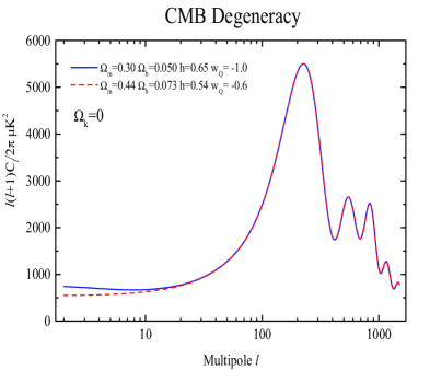
FIG. 1.: CMB power spectra and the angular diameter distance degeneracy. The models are computed assuming flatness, $\Omega_{k}=1-\Omega_{M}-\Omega_{Q}=0$). The Integrated Sachs Wolfe effect on large angular scale slightly breaks the degeneracy. The degeneracy can be broken with a strong prior on $h$, in this paper we use the results from the HST.

Secondly, the time-varying Newtonian potential after decoupling will produce anisotropies at large angular scales through the Integrated Sachs-Wolfe (ISW) effect. The curve in the CMB angular spectrum on large angular scales depends not only on the value of $w_{Q}$ but also its variation with redshift. However, this effect will be difficult to disentangle from the same effect generated by a cosmological constant, especially in view of the affect of cosmic variance and/or gravity waves on the large scale anisotropies.

In order to emphasize the importance of degeneracies between all these parameters while analyzing the CMB data, we plot in Figure 1 some degenerate spectra, obtained keeping the physical density in matter $\Omega_{M}h^{2}$, the physical density in baryons $\Omega_{b}h^{2}$ and ${\cal R}$ fixed. As we can see from the plot, models degenerate in $w_{Q}$ can be constructed. However, as we will utilise in the next sections, the combination of the different datasets can break the mentioned degeneracies.

To constrain $w_{Q}$ from CMB, we perform a likelihood analysis comparing the recent CMB observations with a set of models with cosmological parameters sampled as follows: $0.1<\Omega_{m}<1.0$, $-1.0\leq w_{Q}\leq-0.55$, $0.015<\Omega_{b}<0.20$; $0<\Omega_{Q}<0.9$ and $0.45<h<0.95$. We vary the spectral index of the primordial density perturbations within the range $n_{s}=0.60,...,1.40$, we allow for a possible reionization of the intergalactic medium by varying the CMB photons optical depth in the range $0.0<\tau_{C}<0.4$ and we re-scale the fluctuation amplitude by a pre-factor $C_{10}$, in units of $C_{10}^{COBE}$. We also restrict our analysis to flat models, $\Omega_{tot}=1$, and we add a conservative external prior on the age of the universe $t_{0}>10$ Gyrs (see e.g. [24]).

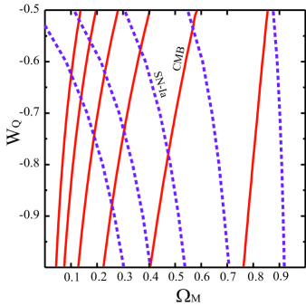
FIG. 2.: Contours of constant $R$ (CMB) and $SN-Ia$ luminosity distance in the $w_{Q}$-$\Omega_{M}$ plane. The degeneracy between the two distance measures can be broken by combining the two sets of complementary information. The luminosity distance is chosen to be equal to $d_{l}$ at $z=1$ for a fiducial model with $\Omega_{\Lambda}=0.7$, $\Omega_{M}=0.3$,$h=0.65$. (We note that as $\Omega_{Q}=1-\Omega_{M}$ goes to zero the dependence of $R$ and $d_{L}$ upon $w_{Q}$ also become zero, as there is no dark energy present.)

In order to speed-up the computation time of the theoretical models for different $w_{Q}$ we make use of a $k$-splitting technique [20]. Basically a $w_{Q}=-1$ and $w_{Q}>-1$ model are calculated in two different ways. For low $\ell$ the 2 models are computed in the ordinary way by solving the Boltzmann equation, in order to properly take in to account the ISW effect. For the high $\ell$ just a flat, $w_{Q}=-1$ model is calculated. This $w_{Q}=-1$ model is then shifted using the expression for the angular diameter distance in equation (1) to obtain the $w_{Q}>-1$ models.

The theoretical models are computed using a modified version of the publicly available cmbfast program ([22]) and are compared with the recent BOOMERanG-98, DASI and MAXIMA-1 results. The power spectra from these experiments were estimated in $19$, $9$ and $13$ bins respectively, spanning the range $25\leq\ell\leq 1100$. We approximate the experimental signal $C_{B}^{ex}$ inside the bin to be a Gaussian variable, and we compute the corresponding theoretical value $C_{B}^{th}$ by convolving the spectra computed by CMBFAST with the respective window functions. When the window functions are not available, as in the case of Boomerang-98, we use top-hat window functions. The likelihood for a given cosmological model is then defined by $-2{\rm ln}{\cal L}=(C_{B}^{th}-C_{B}^{ex})M_{BB^{\prime}}(C_{B^{\prime}}^{th}-C_{B^{\prime}}^{ex})$ where $C_{B}^{th}$ ($C_{B}^{ex}$) is the theoretical (experimental) band power and $M_{BB^{\prime}}$ is the Gaussian curvature of the likelihood matrix at the peak. We consider $10\%$, $4\%$ and $4\%$ Gaussian distributed calibration errors (in $\mu K$)for the BOOMERanG-98, DASI and MAXIMA-1 experiments respectively and we take in to account for the beam error in BOOMERanG-98 by analytic marginalization as in [23]. We also include the COBE data using Lloyd Knox’s RADPack packages.

Constraints from Supernovae. Evidence that the universe’s expansion rate was accelerating was first provided by two groups, the SCP and High-Z Search Team([1]) using type Ia supernovae (SN-Ia) to probe the nearby expansion dynamics. SN-Ia are good standard candles, as they exhibit a strong phenomenological correlation between the decline rate and peak magnitude of the luminosity. The observed apparent bolometric luminosity is related to the luminosity distance, measured in Mpc, by $m_{B}=M+5logd_{L}(z)+25$. where M is the absolute bolometric magnitude. The luminosity distance is sensitive to the cosmological evolution through an integral dependence on the Hubble factor $d_{l}=(1+z)\int_{0}^{z}(dz^{\prime}/H(z^{\prime},\Omega_{Q},w_{q})$ and therefore can be used to constrain the scalar equation of state. We evaluate the dark energy $\Omega/w$ likelihoods assuming a constant equation of state, such that $H(z)=\rho_{0}\sum_{i}\Omega_{i}(1+z)^{(3+3w_{i})}$. The predicted $m_{eff}$ is then calculated by calibration with low-z supernovae observations [25] where the Hubble relation $d_{l}\approx H_{0}cz$ is obeyed. We calculate the likelihood, ${\cal L}$, using the relation ${\cal L}={\cal L}_{0}\exp(-\chi^{2}(\Omega,w_{Q})/2)$ where ${\cal L}_{0}$ is an arbitrary normalisation and $\chi^{2}$ is evaluated using the observations of the SCP group, marginalising over $H_{0}$. As can be seen in Figure 2 there is an inherent degeneracy in the luminosity distance in the $\Omega_{M}/w_{Q}$ plane; one can see that little can be found out about the equation of state from luminosity distance data alone. However, the degeneracies of CMB and SN1a data complement one another so that together they offer a more powerful approach for constraining $w_{Q}$.

TABLE I.: Constraints on $w_{Q}$ and $\Omega_{M}=1-\Omega_{Q}$ using different priors and datasets. We always assume flatness and $t_{0}>10$ Gyr. The $1\sigma$ limits are found from the 16% and 84% integrals of the marginalized likelihood. The HST prior is $h=0.72\pm 0.08$ while for the BBN prior we use the conservative bound $\Omega_{b}h^{2}=0.020\pm 0.005$.

CMB+HST	$w_{Q}<-0.62$
	$0.15<\Omega_{M}<0.45$
CMB+HST+BBN	$-0.95<w_{Q}<-0.62$
	$0.15<\Omega_{M}<0.42$
CMB+HST+SN-Ia	$-0.94<w_{Q}<-0.74$
	$0.16<\Omega_{M}<0.34$
CMB+HST+SN-Ia+LSS	$w_{Q}<-0.85$
	$0.28<\Omega_{M}<0.43$

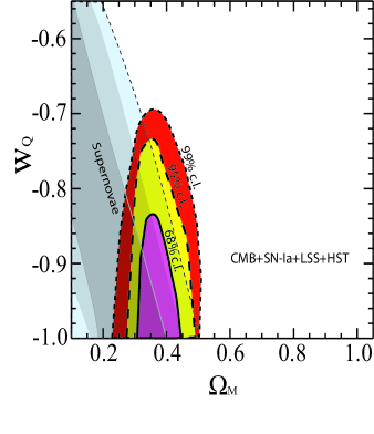
FIG. 3.: The likelihood contours in the ($\Omega_{M}$, $w_{Q}$) plane, with the remaining parameters taking their best-fitting values for the joint CMB+SN-Ia+LSS analysis described in the text. The contours correspond to 0.32, 0.05 and 0.01 of the peak value of the likelihood, which are the 68%, 95% and 99% confidence levels respectively.

Results. Table I shows the $1$-$\sigma$ constraints on $w_{Q}$ for different combinations of priors, obtained after marginalizing over all remaining nuisance parameters. The analysis is restricted to flat universes. One can see that $w_{Q}$ is poorly constrained from CMB data alone, even when the HST strong prior on the Hubble parameter, $h=0.72\pm 0.08$, is assumed. Adding a Big Bang Nucleosynthesis prior, $\Omega_{b}h^{2}=0.020\pm 0.005$, has small effect on the CMB+HST result. Adding SN-Ia breaks the CMB $\Omega_{Q}-w_{Q}$ degeneracy and improves the upper limit on $w_{Q}$, with $w_{Q}<-0.74$. Finally, including information from local cluster abundances through $\sigma_{8}=(0.55\pm 0.1)\Omega_{M}^{-0.5}$, where $\sigma_{8}$ is the rms mass fluctuation in spheres of $8h^{-1}$ Mpc, further breaks the quintessential-degeneracy, giving $w_{Q}<-0.85$ at $1$-$\sigma$. Also reported in Table I, are the constraints on $\Omega_{M}$. As we can see, the combined data suggests the presence of dark energy with high significance, even in the case CMB+HST. It is interesting to project our likelihood in the $\Omega_{Q}-w_{Q}$ plane. Proceeding as in [26], we attribute a likelihood to a point in the ($\Omega_{M}$, $w_{Q}$) plane by finding the remaining parameters that maximise it. We then define our $68\%$, $95\%$ and $99\%$ contours to be where the likelihood falls to $0.32$, $0.05$ and $0.01$ of its peak value, as would be the case for a two dimensional multivariate Gaussian. In Figure 3 we plot likelihood contours in the ($\Omega_{M}$, $w_{Q}$) plane for the joint analyses of CMB+SN-Ia+HST+LSS data together with the contours from the SN-Ia dataset only. As we can see, the combination of the data breaks the luminosity distance degeneracy.

Constraining dynamical models. In the previous section we obtained bounds on the equation of state parameter $w_{Q}$ by assuming it is a constant, independent of the redshift. However, in quintessential models the equation of state can vary with time. It is therefore useful to discuss how well our constraints on $w_{Q}$ apply to less trivial models. There are a wide variety of quintessential models; we illustrate our analysis using representatives of three of the most general classes of model: the inverse power law,$V(\phi)=V_{0}/\phi^{p}$ [3] with p=1, an exponential scaling potential with a feature, $V(\phi)=V_{0}e^{-\lambda\phi}(A+(\phi-\phi_{0})^{2})$ [18], with $\lambda=10,A=0.008,\phi_{0}=25.8$, and an oscillatory scaling potential,$V(\phi)=V_{0}e^{-\lambda\phi}(1+Asin(\nu\phi))$ [27] with $\lambda=4,A=0.98,\nu=0.51$. In each case $V_{0}$ is chosen so that $\Omega_{Q}=0.7$ and $H_{0}$ is 65. The particular time dependent characteristics of each are shown in Figure 4.

FIG. 4.: The variation of $\Omega_{Q}$ and $w_{Q}$ with redshift for the three models described in section V. The power law potential (full line) $w_{Q}$ shows a steady small variation, the exponential feature potential, (short dashed line) acts remarkably like a cosmological constant at late times, after a deviation from behaving like normal matter with $w_{Q}\sim 0$, whilst the oscillating potential (dot-dash) shows a continual variation in $w_{Q}$.

If we are to constrain dynamical models, we need to understand how well the effect of a time varying $w_{\phi}$ can be modeled by a constant $w_{eff}$. In [28] it was shown that in models in which the dark energy component is negligible at last scattering, the CMB and matter power spectra are well approximated by $w_{eff}=\int da\Omega_{Q}(a)w_{Q}(a)$. This is demonstrated in figure 5 in the case of the exponential potential with a feature, using $w_{eff}=-0.993$. In [19] we showed that if the dark energy component is a significant proportion, as can be seen in scaling quintessence models, the dark energy component can be modelled as an additional contribution to the effective number of relativistic degrees of freedom. We restrict ourselves to former case in which $\Omega_{\phi}(MeV)$ is negligible. In [13] it is noted that although $w_{eff}$ is a good measure for modelling CMB spectra it may not be such a good measure when considering $d_{l}$. We investigate whether this is actually the case using the three models outlined above, a power law, exponential scaling and scaling oscillatory potential, as test cases. In Figure 6 we show that even a substantial deviation from $w_{eff}$ at late times produces a small change in $\rho_{Q}$. The effect on $m_{B}$ is doubly ‘numbed’, firstly because of the smoothing by the integral relation with $H$ in $d_{l}$, see [14] for a previous discussion of this, and secondly because $m_{B}\sim logd_{l}$. As a result the bolometric magnitude taken from the SN1a data is highly insensitive to variations in the equation of state. This doesn’t bode well if we are to try and reconstruct the time varying equation of state from observations. It looks more likely that $w_{eff}$ will be a more tangible observable.

FIG. 5.: Comparison of CMB temperature power spectra for the dynamical quintessence model with an exponential potential with a feature described in section V, and a model with constant $w_{Q}=w_{eff}$ for the dynamical model. In both cases with $\Omega_{Q}=0.7$ and $H_{0}=65$. One can see that the constant model is a remarkably good approximation to the dynamical model, despite the equation of state of the dynamical model varying significantly from the effective value from recombination until nowadays.

FIG. 6.: The implication of a deviation $\Delta w_{Q}=1-w_{eff}/w_{Q}$ on $\Delta D_{L}=1-D_{L}(w_{eff})/D_{L}(w_{Q})$ and $\Delta m_{B}=m_{B}(w_{Q})-m_{B}(w_{eff})$ for the three models in section V. The tracker potential (full line) has $w_{eff}=-0.727$, the exponential potential with feature (dashed line) has $w_{eff}=-0.993$ and the oscillatory potential (dot-dash) has $w_{eff}=-0.529$. Notice that $D_{L}$ and $m_{B}$ are in turn both desensitized to any variation in $w_{Q}$.

Conclusions. In this paper we have provided new constraints on the dark energy equation of state parameter $w_{Q}$ by combining different cosmological data. The new CMB results provided by Boomerang and DASI improve the constraints from previous and similar analysis (see e.g., [13],[29]), with $w_{Q}<-0.85$ at $68\%$ c.l. ($w_{Q}<-0.76$ at $95\%$ c.l.). We have also demonstrated how the combination of CMB data with other datasets is crucial in order to break the $\Omega_{Q}-w_{Q}$ degeneracy. The constraints from each single datasets are, as expected, quite broad but compatible between each other, providing an important consistency test. When comparison is possible (i.e. restricting to similar priors and datasets), our analysis is compatible with other recent analysis on $w_{Q}$ ([31]). Our final result is perfectly in agreement with the $w_{Q}=-1$ cosmological constant case and gives no support to a quintessential field scenario with $w_{Q}>-1$. A frustrated network of domain walls or a purely exponential scaling field are excluded at high significance. In addition a number of quintessential models are highly disfavored, power law potentials with $p\geq 1$ and the oscillatory potential discussed in this paper, to name a few.

It will be the duty of higher redshift datasets, for example from clustering observations [30] to point to a variation in $w$ that might place quintessence in a more favorable light.

The result obtained here, however, could be plagued by some of the theoretical assumptions we made. The CMB and LSS constraints can be weakened by the inclusion of a background of gravity waves or of isocurvature perturbations or by adding features in the primordial perturbation spectra. These modifications are not expected in the most basic and simplified inflationary scenario but they are still compatible with the present data. The SN-Ia result has been obtained under the assumption of a constant-with-time $w_{Q}$. We have shown that in general $w_{eff}$ is a rather good approximation for dynamical quintessential mode ls since the luminosity distance depends on $w_{Q}$ through a multiple integral that smears its redshift dependence. As we show in the previous section, our result is therefore valid for a wide class of quintessential models. This ‘numbing’ of sensitivity to $w_{Q}$ implies that maybe an effective equation of state is the most tangible parameter able to be extracted from supernovae. However with the promise of large data sets from Planck and SNAP satellites, opportunities may yet still be open to reconstruct a time varying equation of state [16].

Acknowledgements It is a pleasure to thank Ruth Durrer, Steen Hansen and Matts Roos for comments and suggestions. RB and AM are supported by PPARC. We acknowledge the use of CMBFAST [22].

REFERENCES

- [1] P.M. Garnavich et al, Ap.J. Letters 493, L53-57 (1998); S. Perlmutter et al, Ap. J. 483, 565 (1997); S. Perlmutter et al (The Supernova Cosmology Project), Nature 391 51 (1998); A.G. Riess et al, Ap. J. 116, 1009 (1998); B.P. Schmidt, Ap. J. 507, 46-63 (1998).
- [2] N. Bahcall, J. P. Ostriker, S. Perlmutter and P. J. Steinhardt, Science 284, 1481 (1999) [astro-ph/9906463]; A. H. Jaffe et al,Phys. Rev. Lett. 86 (2001) [astro-ph/0007333].
- [3] I. Zlatev, L. Wang, & P. Steinhardt, Phys. Rev. Lett. 82 896-899 (1999).
- [4] P. Brax, J. Martin & A. Riazuelo, Phys. Rev. D.,62 103505 (2000).
- [5] C Wetterich, Nucl. Phys B. 302 668 (1988)
- [6] B. Ratra and J. Peebles, Phys. Rev D37 (1988) 321.
- [7] J. Frieman, C. Hill, A. Stebbins, I. Waga, Phys. Rev. Lett, 75 2077 (1995).
- [8] P. Ferreira and M. Joyce, Phys.Rev. D58 (1998) 023503.
- [9] C.B. Netterfield et al., [astro-ph/0104460].
- [10] C. Pryke et al., [astro-ph/0104489].
- [11] A. Lee et al., [astro-ph/0104459].
- [12] Freedman W. L. et al, 2000, ApJ in press, preprint astro-ph/0012376.
- [13] S. Perlmutter, M.S. Turner, M. White, Phys.Rev.Lett. 83 670-673 (1999).
- [14] I. Maor, R. Brustein, P.J. Steinhardt, Phys.Rev.Lett. 86 (2001) 6
- [15] W. Hu, astro-ph/9801234.
- [16] J. Weller, A. Albrecht, Phys.Rev.Lett. 86 1939 (2001) [astro-ph/0008314]; D. Huterer and M. S. Turner, [astro-ph/0012510]; M. Tegmark, [astro-ph/0101354].
- [17] M. Doran, M. Lilley, C. Wetterich, [astro-ph/0105457]
- [18] A. Albrecht,C. Skordis, Phys.Rev.Lett. 84 2076 (2000) [astro-ph/9908085]; C. Skordis, A . Albrect, Phys. Rev. D, Submitted [astro-ph/0012195].
- [19] R. Bean, S. H. Hansen, A. Melchiorri, PRD in press, [astro-ph/0104162].
- [20] M. Tegmark, M. Zaldarriaga, A. Hamilton, Phys.Rev. D63 (2001) 043007, astro-ph/0008167.
- [21] G. Efstathiou & J.R. Bond [astro-ph/9807103]; A. Melchiorri & L. M. Griffiths, New Astronomy Reviews, 45, 4-5, 2001, [astro-ph/0011197].
- [22] M. Zaldarriaga & U. Seljak, ApJ. 469 437 (1996).
- [23] S. Bridle et al., in preparation.
- [24] I. Ferreras, A. Melchiorri, J. Silk, MNRAS 327, L47 (2001), [astro-ph/0110472].
- [25] M. Hamuy, Astron. J. 106,2392 (1993)
- [26] A. Melchiorri et al., Astrophys.J. 536 (2000) L63-L66, astro-ph/9911445.
- [27] S. Dodelson, M. Kaplinghat and E. Stewart, Phys. Rev. Lett. 85 (2000) 5276 [astro-ph/0002360].
- [28] G. Huey, L.Wang, R. Dave, R. R. Caldwell, P. J. Steinhardt, Phys.Rev. D59 (1999) 063005
- [29] J. R. Bond et al. [The MaxiBoom Collaboration], astro-ph/0011379.
- [30] M.O. Calvão, J.R.T De Mello Neto& I. Waga [astro-ph/0 107029], J. Newman, C. Marinoni, A. Coil & M. Davis [astro-ph/0109131], T. Matsubara & A. Szalay [astro-ph/0105493].
- [31] C. Baccigalupi, A. Balbi, S. Matarrese, F. Perrotta, N. Vittorio, astro-ph/0109097; P.S. Corasaniti & E.J. Copeland, astro-ph/0107378; T. Saini, S. Raychaudhury, V. Sahni and A.A. Starobinsky, Phys. Rev. Lett. 85, 1162 - 1165 (2000); Y. Wang, G. Lovelace, astro-ph/0109233.