Temperature Profiles of Nearby Clusters of Galaxies

Abstract

We report results from the analysis of 21 nearby galaxy clusters, 11 with cooling flow (CF) and 10 without cooling flow, observed with BeppoSAX. The temperature profiles of both CF and non-CF systems are characterized by an isothermal core extending out to $\sim 0.2~{}r_{180}$; beyond this radius both CF and non-CF cluster profiles rapidly decline. Our results differ from those derived by other authors who either found continuously declining profiles or substantially flat profiles. Neither the CF nor the non-CF profiles can be modeled by a polytropic temperature profile, the reason being that the radius at which the profiles break is much larger than the core radius characterizing the gas density profiles. For $r>0.2~{}r_{180}$, where the gas can be treated as a polytrope, the polytropic indices derived for CF and non-CF systems are respectively $1.20\pm 0.06$ and $1.46\pm 0.06$. The former index is closer to the isothermal value, 1, and the latter to the adiabatic value, 5/3. Published hydrodynamic simulations do not reproduce the peculiar shape of the observed temperature profile, probably suggesting that a fundamental ingredient is missing.

1 Introduction

Galaxy clusters, being the largest virialized systems in the universe, are useful cosmological probes. Through the assumption of hydrostatic equilibrium for the X-ray emitting intra-cluster medium (ICM) it is possible to measure the total gravitational mass of clusters (including the dominating dark matter component) as a function of the gas temperature and density profiles.

Current models of structure formation suggest that the mass components of clusters are representative of the universe as a whole. Once the gas mass is determined from X-ray data in the deprojection or fitting analysis (see e.g. Fabian et al. 1981; Ettori & Fabian 1999) and the total mass is estimated through the hydrostatic equilibrium, it is possible to derive the gas fraction. This fraction is a lower limit on the global baryon fraction and can be used to constrain the cosmological density parameter if combined with primordial nucleosynthesis calculations (e.g. White et al. 1993). If well calibrated, the slope and evolution of cluster scaling relations, such as the gas mass vs. temperature (e.g. Finoguenov, Reiprich & Böhringer 2001; Voit 2000) and the cluster size vs. temperature (e.g. Mohr et al. 2000; Verde et al. 2001), can be used to constrain cosmological and structure formation models . For instance, the mass-temperature relation is fundamental in linking theoretical cosmological models, which give the mass function of clusters via the Press-Schechter formalism, and the observed temperature function (e.g. Henry 1997; Nevalainen, Markevitch & Forman 2000). Temperature profiles are also fundamental in determining the gas entropy distribution (see Lloyd-Davies, Ponman & Cannon 2000 and references therein), which is a powerful tool to explore non-gravitational processes that could alter the specific thermal energy in the ICM, such as pre-heating of the gas before it falls into the cluster core and energy injection from supernova-driven galaxy winds.

While ROSAT X-ray images allowed high-precision studies of the gas density distribution in individual clusters (e.g. Mohr, Mathiensen & Evrard 1999), spatially resolved temperature measurements have only become possible recently with ASCA and BeppoSAX. With previous missions (e.g. HEAO1, Einstein, EXOSAT, Ginga) only global temperature measurements were available and therefore the ICM was assumed to be roughly isothermal. ROSAT was not the ideal instrument to measure temperature structures in rich clusters given its soft spectral range (0.1-2.4 keV), nonetheless various attempt have been made in the last years for a few very bright clusters (e.g. Briel & Henry 1994, 1996; Knopp, Henry & Briel 1996; Davis & White 1998) or using color ratios techniques (Irwin, Bregman & Evrard 1999; Sanders, Fabian & Allen 2000).

Different studies have found conflicting results regarding temperature gradients in clusters. In 1998 Markevitch and collaborators (hereafter MFSV98) analyzed azimuthally averaged radial temperature profiles for 30 clusters observed with ASCA, finding that nearly all clusters show a significant radial temperature decline at large radii. By fitting the composite temperature profile for symmetric clusters with a polytropic relation up to $\sim 55\%$ of the virial radius, MFSV98 found that the temperature decline corresponded to a polytropic index of $\sim 1.24$ on average. However, doubts on the universality and the steepness of this profile have been raised by subsequent studies. Irwin et al. (1999) comparing the MFSV98 results with the work from other authors (see references in Irwin et al. 1999), found isothermal temperature profiles, even for those clusters where MFSV98 found a temperature decline. Moreover, from an investigation of ROSAT PSPC color profiles, they found that clusters were generally isothermal, even in clusters in common with the MFSV98 analysis. After the analysis of a sample of 106 clusters observed with ASCA, White (2000) concluded that $90\%$ of the temperature profiles were consistent with being flat. For a sample of cool clusters (i.e. kT$\lesssim 4$ keV) Finoguenov et al. (2001) derived ASCA/SIS temperature profiles similar to the universal temperature profile of MFSV98, although the radial range explored by these authors was smaller than that studied by MFSV98.

Although ASCA has been the first X-ray instrument able to perform spatially resolved spectroscopy in hot clusters given its adequate energy range (1-10 keV), its large and strongly energy-dependent point-spread function (PSF) required complicated correction procedures for the spectral analysis of extended sources. Different works on temperature measurements with ASCA have applied different methods to correct for the PSF effects. In this respect BeppoSAX (Boella et al. 1997a) is a more suitable instrument to investigate temperature structures in galaxy clusters and supplies an independent dataset with respect to ASCA. The Medium-Energy Concentrator Spectrometer (MECS; Boella et al. 1997b) on board BeppoSAX works in a similar energy range of ASCA, but has a sharper PSF (HPR $\sim 1^{\prime}$), which is radially symmetric and almost energy independent (D’Acri, De Grandi & Molendi 1998).

Recent results for several nearby clusters (e.g. A2319: Molendi et al. 1999; A3266: De Grandi & Molendi 1999a; A2256: Molendi, De Grandi & Fusco-Femiano 2000; A3562: Ettori et al. 2000; A3571: Nevalainen et al. 2001; etc.) show that BeppoSAX has the ability to obtain better constraints than ASCA on temperature profiles. Irwin & Bregman (2000) (hereafter IB00), who analyzed a sample of 11 clusters observed with BeppoSAX, placed further arguments supporting a general isothermality of the ICM. IB00 claimed that the temperature profiles were generally flat or increase slightly out to $\sim 30\%$ of of the virial radius.

In this paper we investigate radial cluster temperature profiles for a sample which doubles the IB00 sample using new archival and proprietary BeppoSAX data. Contrary to IB00, who limited the analysis within $9^{\prime}$ (i.e. to regions $\lesssim 30\%$ of the virial radius), we will consider the full field of view of the MECS in order to extend our radial temperature analysis out to $\sim 50\%$ or more of the virial radius (i.e. to radii comparable to those explored by MFSV98 and White 2000). Using an independent dataset from ASCA we are interested in searching if temperature declines are a common phenomena in clusters, and if this is the case, what is the typical shape or gradient. We will also test if declines are specific to certain types of systems.

The plan of this paper is as follows. In Section 2 we describe the sample. In Section 3 we present the BeppoSAX observations and discuss in details the X-ray data analysis, the spectral modeling is presented in $\S$ 3.1 and a technical comparison with the IB00 sample is in $\S$ 3.2. In Section 4 we investigate the projected temperature profiles derived for our sample, in $\S$ 4.1 we test the temperature profiles at large radii for instrumental or systematic effects, in $\S$ 4.2 and 4.3 we apply various models to the profiles and discuss some implication of the results. In Section 5 we compute the averaged cluster temperature profiles and compare them to previous measures ($\S$ 5.1), to XMM-Newton observations ($\S$ 5.2) and to hydrodynamical cluster simulations ($\S$ 5.3). A summary of our main conclusions is given in Section 6.

Quoted confidence intervals are $68\%$ for 1 interesting parameter (i.e. $\Delta\chi^{2}=1$), unless otherwise stated. We use $H_{o}=50$ Mpc km s^-1 and $q_{o}=0.5$.

2 The Sample

The aim of this paper is to derive spatially resolved temperature measurements for a sample of rich and nearby (i.e., $0.02\lesssim z\lesssim 0.1$) clusters of galaxies observed with the BeppoSAX satellite and to investigate the possible existence of an universal temperature profile for rich clusters. We selected all the clusters with on-axis pointings and exposure times larger than 30 ks which were available at the BeppoSAX SDC archive at the end of March 2001 (including a few proprietary observations).

We have divided the sample of the 21 selected clusters into a subsample of 10 non-cooling flow (non-CF) and 11 cooling flow (CF) objects on the basis of the ROSAT analysis presented in Peres et al. (1998), defining a non-CF cluster an object with a mass deposition rate consistent with zero.

Our redshift range allows us to explore in details the innermost regions of a few nearby clusters (i.e. Coma, A1367, Perseus and A3627) out to $\sim 20\%$ of the virial radius, and to measure temperatures out to $\sim 50\%$ of the virial radius for the other clusters in the sample.

A detailed discussion of the metal abundance profiles derived for a subset of 17 clusters of this sample is presented in De Grandi & Molendi (2001). In a forthcoming paper (Ettori et al. 2001 in prep.) we will discuss the mass profiles derived for this sample. The observation log for the current cluster sample is given in Table 1.

3 Data Analysis

In this paper we have considered observations from the MECS on board BeppoSAX. The MECS is presently composed by two units working in the 1-10 keV energy range, with energy resolution $\sim 8\%$ and angular resolution $\sim 0.7^{\prime}$ (FWHM), both computed at 6 keV.

For each cluster we have analyzed the data from the MECS2 and MECS3 separately. Standard reduction procedures and screening criteria have been applied using the SAXDAS package under FTOOLS environment to produce equalized and linearized MECS event files. Using the information contained in the housekeeping files we have rejected all events which have occurred at times when the instantaneous pointing direction differed by more than $10^{\prime\prime}$ from the mean pointing direction.

The PSF of the MECS instrument is known to vary only weakly with energy (D’Acri et al. 1998). Although we expect PSF-induced spectral distortions to be small, we have properly taken them into account creating corrected effective area files with the EFFAREA program available within the SAXDAS package. This program convolves the ROSAT PSPC surface brightness profile, computed from archival PSPC pointings data, with an analytic model of the MECS PSF to estimate spectral distortions. EFFAREA also includes corrections for the energy-dependent telescope vignetting for on-axis observations.

Each cluster has been divided into concentric annuli centered on the X-ray emission peak. Out to $8^{\prime}$ we accumulated spectra from 4 annular regions each $2^{\prime}$ wide, beyond this radius we accumulated spectra from annuli $4^{\prime}$ wide. Whenever it is necessary we exclude pointlike sources along the line of sight by excising a circular region with radius $2^{\prime}$. For each cluster the radial profile stops at the last annulus containing more than $30\%$ source counts with respect to the total (i.e. source$+$background) counts. The dominant contribution to the MECS background at energies larger than $\sim$ 5 keV is from events induced by the interaction of high energy particles with the structure surrounding the instrument. Using data acquired during occultations of the satellite from the dark earth, Vecchi et al. (1999) have monitored the non X-ray background finding that variations are typically contained within $\sim 5\%$ from the mean. In the present work, we have decided to account for these variations by excluding from our analysis spectra from the outermost regions not satisfying the conditions on the intensity of the source with respect to the background indicated above. We believe that this is preferable to the alternative choice of using this data and including a systematic component to the error budget to account for possible variations in the background, the reason being that if such a component exists and is truly systematic it will show up again when we average our profiles. For the spectra which satisfy the conditions on the intensity of the source with respect to the background indicated above, fluctuations of the background of up to $\sim 5\%$ do not introduce a significant increase in the error of the temperature measurement.

The energy range used for the spectral fitting is 2-10 keV with the exceptions described in the following. In the outermost annuli if the source counts drops to less than $50\%$ with respect to the total counts, we restrict the energy range to 2-8 keV, to avoid possible distortions from the hard MECS instrumental background (see the above discussion).

One of the most important steps in the MECS data reduction is the correct treatment of the detector entrance window structure. The Beryllium window is sustained by a thicker supporting structure, the so called strongback, in form of a circular ring and four ribs. The transmission of the Be window is function both of the energy (being the prime responsible of the low energy cutoff in the effective area), and position (because of the presence of the strongback). The strongback affects the detector regions covered by its geometrical shadow convolved through the detector PSF and produces an artificial hardening in the spectra accumulated from these regions. Taking into account this convolution the circular ring of the strongback starts at $\sim 8^{\prime}$ and ends at $\sim 12^{\prime}$ from the detector center. We have computed the corrected effective area for the $8^{\prime}-12^{\prime}$ annulus by considering the typical thickness of the strongback and its transmission as a function of the energy and position. Moreover, in the $8^{\prime}-12^{\prime}$ annulus we restrict our analysis to the range 3.5-10 keV to avoid the low energy part of the spectrum where our correction is less reliable. All other regions of the detector covered by the strongback have been appropriately masked and the data rejected. Another problem related to the strongback is that the detector center and the pointing axis of the X-ray telescope are not coincident, and that the distance between these two points, albeit small, is different in MECS2 and MECS3. Thus the same region of an extended source (in sky coordinates) is shadowed by the strongback differently in the two MECS. Therefore, it is important to apply the strongback correction to the effective areas of the two MECS separately.

The background subtraction has been performed using spectra extracted from blank sky events files in the same region of the detector as the source. Total and background spectra and effective areas of the two MECS units have been added together using the FTOOLS mathpha and addarf, respectively.

3.1 Spectral modeling

We have rebinned (FTOOLS grppha) the spectra to collect a minimum of 25 counts in each energy bin to allow the use of the $\chi^{2}$ analysis. All spectral fits have been performed using XSPEC version 10.00.

We fit each observed spectra with a thermal emission model for a low-density plasma in collisional ionization equilibrium (mekal model in XSPEC), absorbed by the nominal Galactic column density (Dickey & Lockman 1990; wabs model). This model assumes thermal emission at a single temperature and is characterized by three free parameters, the gas temperature, the metal abundance given relative to the solar value, and the normalization. We find that freeing the redshift to account for the systematic shift of $\sim 40$ eV in the MECS conversion from channel to energy affect the temperature measurements by less than $5\%$ (in agreement with the analysis of IB00).

Recent observations from Chandra (Hydra A: David et al. 2000) and XMM (M87, A1795 and A1835: Molendi & Pizzolato 2001) X-ray observatories show a lack of spectroscopic evidence for multiphase gas in the core of cooling flow clusters. Therefore we will not apply the multiphase models that we (e.g. De Grandi & Molendi 1999b; Molendi & De Grandi 1999) and others (e.g. Allen et al. 2001 and references therein) have used in the past, and will use single temperature models for all regions.

3.2 Comparison with another BeppoSAX sample

We compare here the results on radial temperature profiles derived by Irwin & Bregman (2000) (IB00) from another sample of galaxy clusters observed with BeppoSAX. This sample consists of 11 clusters found in the BeppoSAX archive, 9 of which are in common with our sample. We will concentrate in this Section on the technical differences between our X-ray data analysis and that performed by IB00. A comparison between the scientific results is presented in Section 5.1.

The analysis performed by IB00 differs from ours in several respects. The most important difference is that these authors limit the radial analysis at a radius of $9^{\prime}$, whereas our analysis considers the whole useful detector area up to $20^{\prime}$. The second difference is that IB00 do not correct the data for the strongback effect, claiming that this effect becomes a factor only at radii larger than $9^{\prime}$.

This is not the case because the strongback starts effecting the spectra at about 8^′ from the center of the detector and also because the center of the cluster can be offset by up to 2^′ from the center of the detector (for further details see Section 3). Finally, they do not investigate the difference between CF and non-CF clusters in such a systematic way as we do.

IB00 find that the temperature profiles of their clusters are generally flat, or increase slightly out to $\sim 30\%$ of the virial radius and that a decline of the temperature of $14\%$ out to $30\%$ of the virial radius is ruled out at the $99\%$ confidence level. These results appear to be in contradiction with the ones we report in Section 4. To further investigate this difference we have considered three CF clusters in common between our sample and that of IB00 (i.e. A85, A496 and 2A0335$+$096), and we have performed the analysis of the X-ray data in the same way as described in IB00. Namely, we have used the 3.5-10.5 keV energy band and we have not applied any correction for the strongback. As shown in Figure 1, where we compare our results against those of IB00, we are able to reproduce the temperature profiles derived by IB00. We note that the profiles from both analysis are slightly increasing with the radius.

In Figure 2 we compare the temperature profiles for the same three clusters derived using our procedure, which includes a treatment for the strongback (see Section 3 for details), to those of IB00. We find our profiles to be in broad agreement with those of IB00. In all three clusters the temperature measured in the outermost bin by IB00 is slightly larger than the mean temperature of our two overlapping bins. This difference can be most likely attributed to the lack of a proper treatment of the strongback by IB00. Moreover, by extending our analysis further out wee see that the profiles start to decline.

4 Projected Radial Temperature Profiles

In Figure 3 and 4 we present the radial temperature profiles for the non-CF and CF clusters, respectively, plotted against the radius in units of $r_{180}$, which is the radius encompassing a spherical density contrast of 180 with respect to the critical density. In an $\Omega=1$ cosmology this radius approximates the cluster virial radius. We compute $r_{180}$ from the prediction given by the simulations of Evrard, Metzler & Navarro (1996): $r_{180}$ = 3.95 Mpc ($T_{X}/10$ keV)^1/2. Here $T_{X}$ is the mean emission-weighted temperature, in units of keV, which we have estimated by fitting the temperature profile with a constant up to the maximum radius available for each cluster. For the CF clusters we have computed the mean emission-weighted temperature from the temperature profile excluding the cooling flow region (i.e. a central circular region with radius equal or larger than the cooling radius). From the X-ray spatial analysis of Peres et al. (1998) the derived cooling radii of the CF clusters in our sample are generally smaller than 2^′. Exceptions are A2199 and 2A0335$+$096, with cooling radii larger than 2^′ but smaller than 4^′, and the Perseus cluster with a cooling radius of $\sim 6^{\prime}$. For these clusters we have excluded the appropriate cooling flow regions.

In Table 2 we report for each cluster the temperature measurement from each annular region, the mean temperature $T_{X}$ with the corresponding best-fit $\chi^{2}$ and degrees of freedom, the cluster redshift and derived value for $r_{180}$.

4.1 Testing Temperature Profiles at Large Radii

From a visual inspection of Figure 3 and 4 it is evident that a temperature gradient is present at large radii. We have performed a series of checks to test whether this temperature decline is driven by an instrumental or systematic effect.

4.1.1 Criterion on the Outermost Bin

We have applied a more conservative criterion to define the outermost bin for the temperature profiles by imposing that the source counts must exceed $40\%$ (instead of $30\%$ as described in Section 3) of the total counts. By applying this restriction we find that in the case of non-CF clusters the only bin excluded is the last temperature bin of A3266. In the case of CF clusters the outermost bins of 6 clusters (i.e. A1795, A2142, A2199, A3562, 2A0335$+$096 and PKS0745$-$191) are excluded. We have verified that none of the results reported in the next Sections are substantially modified if we reduce the sample by excising the above bins.

4.1.2 Differences between Distant and Nearby Clusters

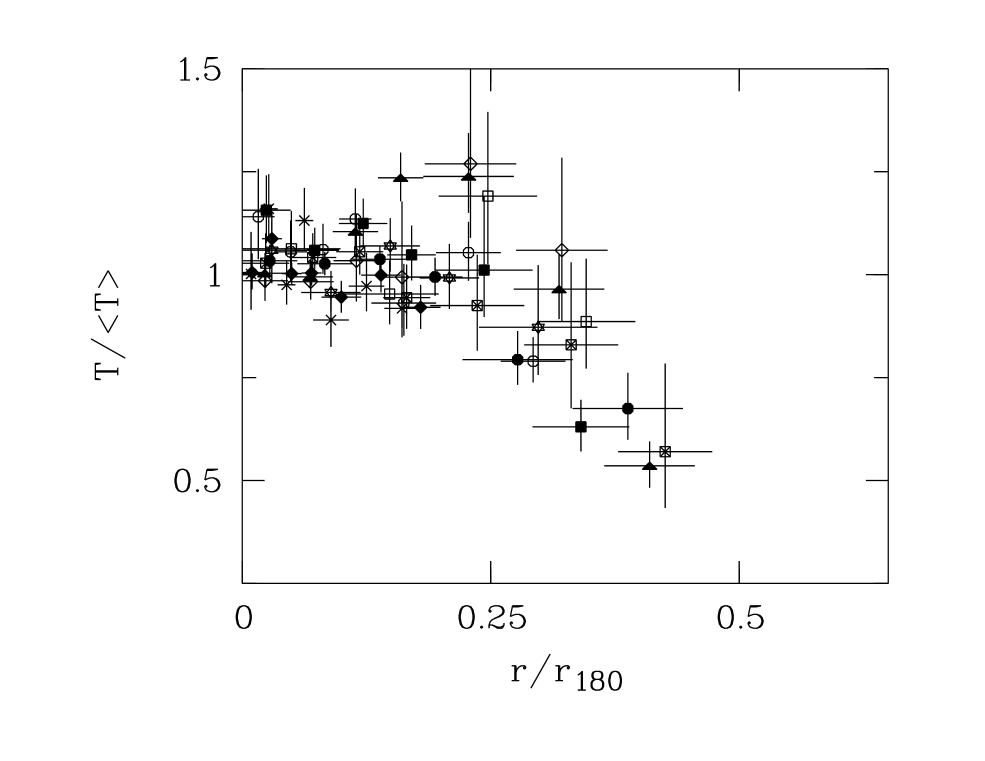
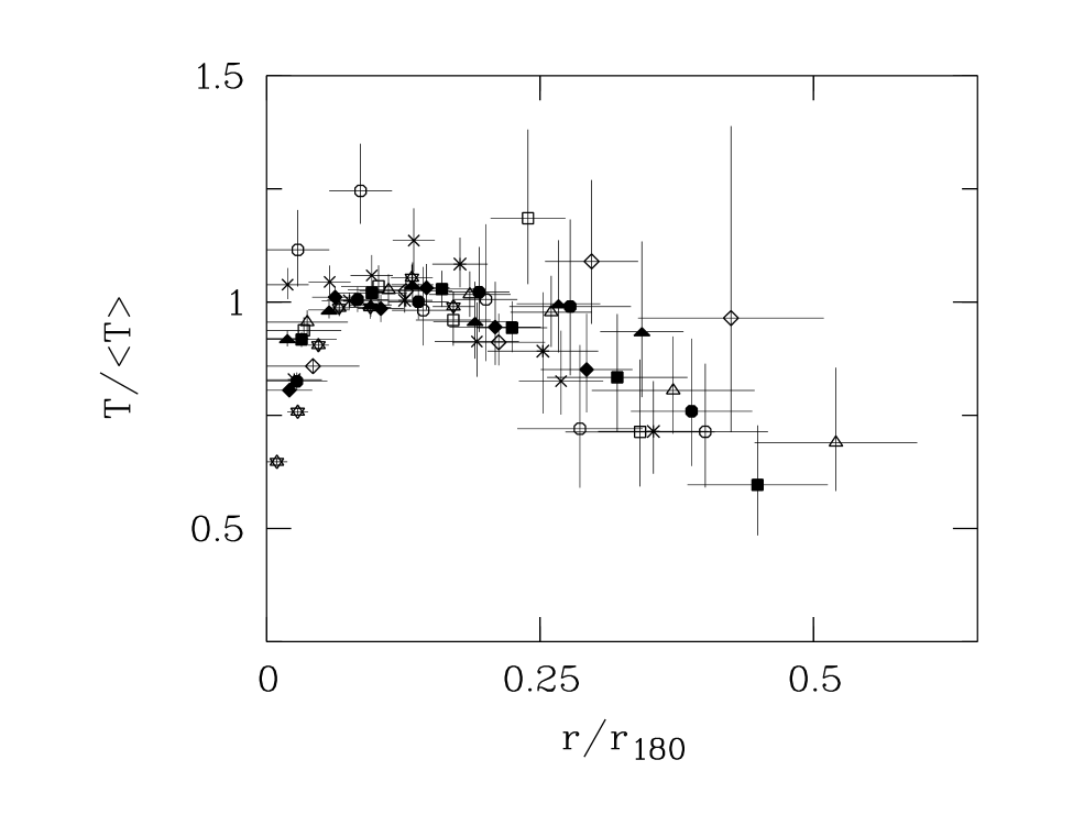
Figure 3: Temperature profiles (projected) for the non-CF clusters, plotted against radii in units of $r_{180}$. Clusters are related to symbols as follows: A119 (filled squares), A754 (filled triangles), A1367 (open circles), A1750 (open squares), A2256 (filled circles), A2319 (open lozenges), A3266 (crossed squares), A3376 (stars), A3627 (crosses) and Coma (filled lozenges).

Figure 4: Temperature profiles (projected) for the CF clusters, plotted against radii in units of $r_{180}$. Clusters are related to symbols as follows: A85 (filled circles), A496 (filled lozenges), Perseus (stars), A1795 (filled squares), A2029 (open squares), A2142 (open triangles), A2199 (filled triangles), A3562 (open circles), A3571 (crosses), 2A 0335$+$096 (asterisks) and PKS 0745$-$191 (open lozenges).

We have plotted in Figure 5 temperature profiles against the radius in arcminutes for four clusters observed at different redshifts. Two of them are nearby cluster, i.e. Coma at z=0.02223 and A3627 at z=0.01628, which are observed by BeppoSAX out to radius of 0.74 Mpc and 0.552 Mpc, respectively. The other two clusters, A119 at z=0.04420 and A2256 at z=0.0570, are more distant and we are able to determine a temperature out to 1.14 Mpc and 1.44 Mpc, respectively. We find that the temperature profiles of the two distant clusters decline with increasing radius, while those of the nearby systems remain constant. This implies that the temperature decline we observe in Figures 3 and 4 is not due to a systematic effect such as, for example, an incorrect vignetting correction at large off-axis angles.

4.1.3 Independent Temperature Measurements for A3562

For one cluster belonging to our sample (A3562) we have two independent BeppoSAX observations, the first one centered on the cluster emission peak and the second one centered on the galaxy group SC 1329$-$313, which is located at about $27^{\prime}$ west of the emission peak of A3562. We find that the two independent measurements of a specific region of A3562 obtained from different parts of the detector give consistent results. More specifically, Ettori et al. (2000) derived the temperature map of A3562 finding a temperature of $3.9^{+1.1}_{-0.8}$ keV in the annulus $8^{\prime}-16^{\prime}$ in the sector pointing towards SC 1329$-$313 (sector west in Figure 9 of Ettori et al. 2000). This temperature is in agreement with the one measured (Bardelli et al. 2001 submitted) from the observation centered on SC 1329$-$313 in the same region (i.e. $3.5\pm 0.3$ keV in the $12^{\prime}-20^{\prime}$ annulus of the north-east sector reported in Bardelli et al. 2001).

4.1.4 Background Subtraction Effects

The increasing importance of background relative to source counts could lead to systematic errors in the measured temperature in the outermost bins. We have performed the following exercise to test this possibility. We have taken the data for the two best-observed clusters that do not show any evidence for a decrease out to $20^{\prime}$ (i.e. Perseus and Coma), and randomly extracted 3.5 ks of data for Perseus and 8 ks for Coma. Similarly, from the blank-sky event files we have randomly extracted 100 ks of data, which we have then added to the 3.5(8) ks of Perseus(Coma) data. In this way we have obtained a simulated “faint” Perseus(Coma) cluster observed for about 100-110 ks. The above exposure times have been chosen so that the number of source counts and the number of source counts with respect to the total counts in the $8^{\prime}-12^{\prime}$, $12^{\prime}-16^{\prime}$, and $16^{\prime}-20^{\prime}$ bins is about the same as in more distant clusters such as A2142, A1795 and A3562. We have repeated this exercise three times for both clusters, each time choosing different chunks of source and background data.

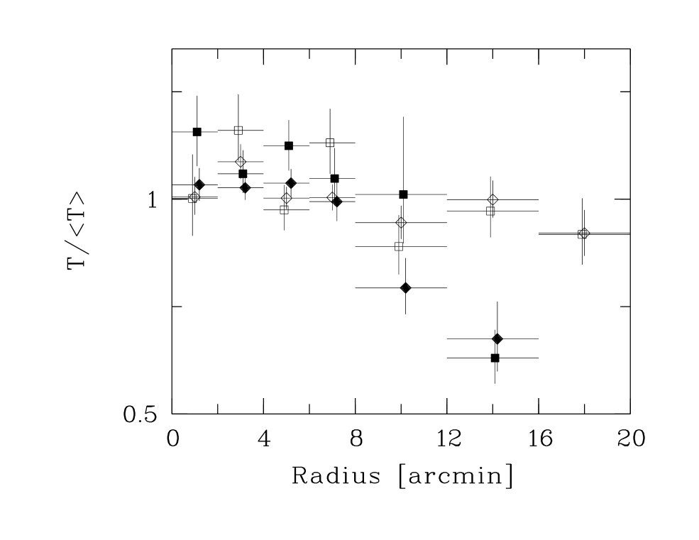
Figure 5: Temperature profile vs. radius in arcminutes for Coma (open lozenges), A3627 (open squares), A119 (filled squares) and A2256 (filled lozenges). Coma and A3627 are nearby clusters at redshift about 0.02, whereas A119 and A2256 are more distant clusters at redshift 0.0442 and 0.0570, respectively.

Figure 6: Temperature profiles vs. radius in arcminutes for “faint” simulated Coma (a) and Perseus (b) clusters (details are given in Section 4.1.4). Filled circles are the original BeppoSAX temperature profiles for Coma and Perseus, open symbols are the profiles resulting from six simulated data sets.

The six simulated data sets have been analyzed like the original data as detailed in Section 3, the resulting temperature profiles for the “faint” Perseus and Coma clusters are shown in Figure 6. We find that these profiles do not show any significant temperature decrement up to the last useful bin indicating that the background subtraction and/or low count rates are not leading to the temperature decline seen in the other clusters of our sample.

4.1.5 PSF and Vignetting correction effects

We have analyzed the clusters in our sample using the corrected and uncorrected on-axis effective areas to check the entity of the PSF and vignetting corrections at all radii and all temperature ranges. In the analysis with the uncorrected effective areas we have not performed any strongback correction in the $8^{\prime}-12^{\prime}$ bin.

In Figure 7 we report the case of Coma, Perseus and A1367 clusters. Let us start by considering the measurements at small radii ($r<8^{\prime}$). In the case of A1367, which has a low temperature and a relatively flat surface brightness profile neither vignetting nor PSF corrections are important. For Perseus which has a somewhat larger temperature and a rapidly declining surface brightness profile the PSF correction slightly increases the temperature for bins from $2^{\prime}$ to $8^{\prime}$. For Coma, which has the highest temperature and almost flat surface brightness profile, where the dominating effect is that of the vignetting, the analysis with the corrected effective areas leads to a slightly larger temperature.

For the $8^{\prime}-12^{\prime}$ bins we always find a higher temperature in the uncorrected effective areas case because of the artificial hardening of the spectrum introduced by the strongback (details are given in Section 3).

At large radii ($r>12^{\prime}$) for low temperature objects such as A1367 no substantial effects are found, for higher temperature objects (Perseus and Coma) the vignetting effect becomes progressively more important, in the case of Perseus ($\sim 7$ keV) the vignetting corrected temperature is $\sim 15-20\%$ higher than the uncorrected one, while for Coma ($\sim 9$ keV) the vignetting corrected temperature is $\sim 20-23\%$ higher than the uncorrected one.

In conclusion, for more then half of the points reported in Figure 7 the correction is smaller than $10\%$, only in the $8^{\prime}-12^{\prime}$ bin and for the outermost bins of hot clusters (kT$>6-7$ keV) the corrections span between $10\%-25\%$.

4.1.6 The Break Radius

As detailed in Section 4.2 our mean temperature profile is well represented by a broken line model (see equation 1). In the following we test whether the break could result from some systematic effect. To this end we have computed, for each cluster, the break radius in arcminutes, $r^{\prime}_{b}$, by fitting the temperature profile (note that the slope of the line was fixed to the mean value, i.e. -2.56 and -1.13, for the non-CF and CF clusters respectively, see Section 4.2 and Table 3). We have then compared $r^{\prime}_{b}$ to $r^{\prime}_{180}$, i.e. $r_{180}$ expressed in arcminutes (see Figure 8). If the break in the profile results from a systematic effect it is likely to occur roughly at the same place in the detector for all clusters, on the contrary if it reflects a genuine property of our objects it will correlate with $r^{\prime}_{180}$. From Figure 8 we see that $r^{\prime}_{b}$ is not the same for all clusters, and that clusters with larger $r^{\prime}_{180}$ tend to have larger $r^{\prime}_{b}$. Indeed, by fitting the data in Figure 8 first with a constant and than with a line we find that the latter fit provides a substantial improvement with respect to the prior (significance $>99.5\%$ according to the F-test).

4.2 Modeling of the Temperature Profiles

We have fitted all the temperature measurements reported in Figure 3 (non-CF clusters), with a constant finding, as expected, that this simple model does not provide a good description of the data (see Table 3). If we try to reproduce the decline observed in Figure 3 by modeling the data with a line we find that the fit improves significantly ($>99.9\%$ according to the F-test). Nonetheless the large $\chi^{2}$ (see Table 3) implies that the fit is still very poor, most likely because the temperature decline is not continuous but begins at a radius of about $0.2~{}r_{180}$. We have therefore modeled our data with a broken line defined as:

$$t=t_{b}\quad{\rm for}~{}x<x_{b}\quad$$

$$t=t_{b}+m*(x-x_{b})\quad{\rm for}~{}x>x_{b}\quad$$

where $t\equiv T/T_{X}$ and $x\equiv r/r_{180}$ are respectively the normalized temperature and radius. The break radius $x_{b}$, the temperature in the isothermal region $t_{b}$, and the slope of the line $m$ for $x>x_{b}$ are the free parameters of the model. This model provides a better description of the data ($>99.9\%$ significance according to the F-test) when compared to the simple line model.

We have performed the same set of fits for the temperature measurements of the CF clusters plotted in Figure 4, results are reported in Table 3. As for the non-CF clusters a line provides a better fit than a constant (significance $>99.9\%$ according to the F-test) and a broken line provides a better fit than a line (significance $>99.9\%$ according to the F-test). Interestingly, while the best fitting $90\%$ confidence for the break radius $x_{b}$ for the two samples overlap, the best fitting slopes $m$ appear to be different at more than the $99.99\%$ confidence level ($5.5\sigma$). Since the break radius and the slope parameter are correlated we have further investigated the difference in $m$ by performing a fit to the non-CF and CF clusters with the value of the break radius fixed at 0.20 (the mean break radius obtained when simultaneously fitting CF and non-CF clusters). The slope for the non-CF clusters is found to be larger at the $99.95\%$ significance level ($3.7\sigma$) than the one for CF clusters, implying that the temperature profile of the former decreases more rapidly than that of the latter. This issue will be discussed in greater detail in Section 4.3.

Given the similarity of the non-CF and CF cluster profiles we have joint the two samples and performed fits to the total sample. Results are reported in Table 3, not surprisingly they are similar to those derived for the two individual subsamples.

4.2.1 The Break Radius

In the following we investigate the properties of the break radii of the individual temperature profiles of our clusters. For each cluster we have computed the break radius by fitting the broken line model described in equation (1), to the temperature profile. We have performed two sets of fits, in the first the slope of the broken line model was fixed to the mean value (i.e. -2.56 for non-CF and -1.13 for CF clusters), while in the second it was left as a free parameter. In the following we use the values of the break radius derived by fixing the slope. By allowing the slope to be a free parameter we find break radii with larger uncertainties with respect to those derived by fixing the slope although the values are consistent each others within $\sim 1\sigma$. This is because the analysis of the individual temperature profiles is often limited by the poor statistics. Note that in the case of Coma, A3627 and A2319, where the profiles are flat, the fitting algorithm pushes the value of the break radius beyond the last data-point. In this case we have fixed the value of the break radius to the radius of the last data-point and have determined the lower bound by varying the break radius until the best fitting $\chi^{2}$ was increased by 1 with respect to the value found by fitting the temperature profile with a constant; the upper bound of the break radius is of course unconstrained. For all profiles with the exception of A754, which is an extremely disturbed and substructured cluster (e.g. Blinton et a. 1998; Henriksen & Markevitch 1996; Zabludoff & Zaritsky 1995), the broken line model provides an acceptable fit to the data, implying that virtually all our profiles can be adequately represented by a broken line model.

The large-scale distribution of the gas temperature in Perseus cluster has been studied with multi-pointing ASCA observations by Ezawa et al. (2001) and Dupke & Bregman (2001). The latter authors derived temperatures from circular regions of $20^{\prime}$ radius at about $40^{\prime}$ from the Perseus cluster emission peak, finding that in the outer regions the gas is roughly isothermal with temperatures of $\sim 6-7$ keV. The profile found by Ezawa et al. (2001) is in agreement with ours out to $20^{\prime}$. In the $20^{\prime}-28^{\prime}$ annular region the authors find a temperature of $\sim 8$ keV, beyond this region their temperature profile shows a smoothly decline of $\sim 2$ keV out to $60^{\prime}$. This decline is similar to what we expect for Perseus on the basis of our broken-line model (i.e. a decline of about 2.5 keV from $20^{\prime}$ to $60^{\prime}$), however the normalization found by Ezawa et al. (2001) is higher by about 1-2 keV.

In Figure 9 we show the break radius in units of $r_{180}$ as a function of redshift for all the objects in our sample. In some cases (e.g. A1367 and 2A0335$+$096) the break radius is well constrained, while in others (e.g. PKS0745$-$191 and A2199) our data does not allow a firm measurement. The mean value of $x_{b}$ is 0.20 with a standard deviation of 0.068. We have performed a statistical test to verify if the above dispersion is due completely to the measurements uncertainties or if it is in part due to an intrinsic dispersion in the distribution of break radii. From the test (Maccacaro et al. 1988), which assumes that the parent population of break radii is distributed like a Gaussian with a mean value, $\overline{x}_{b}$, and an intrinsic dispersion, $\sigma_{x_{b}}$, we find that the intrinsic dispersion is not consistent with zero, $\sigma_{x_{b}}=3.1^{+1.4}_{-0.9}\times 10^{-2}$ (errors are at the $68\%$ confidence limit for one interesting parameter). We conclude that, while the broken line model can adequately fit all our temperature profiles, the break radius is not the same for all objects, although the intrinsic dispersion is relatively small.

Interestingly, if we divide our sample in CF and non-CF cluster and redo the analysis described above, we find that while for CF clusters the intrinsic dispersion is consistent with 0, for non-CF clusters it is not at more than the $99\%$ significance level. Such a difference could result from the fact that CF systems are closer to virialization and therefore more similar one to the other while non-CF systems are irregular and therefore more different one from the other.

4.3 The Polytropic model for the mean Temperature Profile

The broken line model is only a phenomenological model with no physical basis. We have therefore tried comparing our data with a polytropic model. As discussed in Markevitch et al. (1999) and Ettori (2000), under the assumptions that the gas density profile is well represented by a $\beta$-model and that a polytropic relation holds between the gas density and the real three dimensional temperature, the projected temperature profile can be expressed as:

$$t=t_{o}(1+x^{2}/{x_{c}}^{2})^{-1.5\beta(\gamma-1)}$$

where $t\equiv T/T_{X}$, $x\equiv r/r_{180}$, $x_{c}\equiv r_{c}/r_{180}$, $\beta$ is the well known $\beta$ parameter, $\gamma$ is the polytropic index and $t_{o}$ is the normalized temperature at $x=0$. We have assumed a gas distribution with $\beta=2/3$. In the following we describe the application of this model to the mean temperature profile over the full radial range covered by our data.

4.3.1 The full radial range

We performed a first fit leaving $t_{o}$, $x_{c}$ and $\gamma$ as free parameters in equation (2), with the last parameter constrained between the two limiting values of 1 (isothermal gas) and 5/3 (adiabatic gas). The best fit (see Table 4) is found for $\gamma=5/3$ and for $x_{c}=0.48^{+0.04}_{-0.02}$ which, when converted into $r_{c}$ by using the $r_{180}$ value obtained from the mean temperature of the clusters reported in Table 2, yields $r_{c}=1.49^{+0.06}_{-0.13}$ Mpc. This value is unacceptable as it is many times larger than the core radius derived by fitting the surface brightness profiles of galaxy clusters. We have attempted a second fit fixing $x_{c}=0.08$, which corresponds to $r_{c}=0.25$ Mpc. The best fitting value of $\gamma$ is $1.09\pm 0.01$, implying an almost isothermal profile, the $\chi^{2}$ value is large implying that the fit is very poor, indeed the flat model profile does not reproduce the drop observed at radii larger than about 0.2 $r_{180}$. We conclude that the temperature profile for our non-CF clusters is inconsistent with a polytropic temperature model.

The fits with a polytropic law of the CF clusters yield results similar to those found for the non-CF clusters. From the first fit, where $x_{c}$ is a free parameter, we derive a value of $r_{c}$ which is many times larger than the core radius obtained by fitting surface brightness profiles of galaxy clusters. From the second fit we find a best fitting value of $\gamma$ of $1.06\pm 0.01$, implying an almost isothermal profile which, as for the non-CF clusters, does not reproduce the decline observed at radii larger than about 0.2. We note that the $\chi^{2}$ for the second fit is in itself not unacceptable, however, if we compare this fit with the broken line fit, or with the polytropic fit with free $x_{c}$, which are both characterized by a substantial temperature decline at large radii, we find that they provide a significantly better description of the data (in both cases at more than the $99.99\%$ confidence level according to the F-test).

We have also performed fits to the total sample, comprising both non-CF and CF clusters, results are reported in Table 4. In summary our main results are that the polytropic model fails to fit the data adequately and that the broken line model is the one which gives the best description of the data.

4.3.2 The outer regions

Outside about $0.2~{}r_{180}$ both CF and non-CF clusters are characterized by a clear temperature decline. A power-law profile gives acceptable fits for the temperature measurements of CF and non-CF clusters for $r>0.2~{}r_{180}$. The results of the fits, which are reported in Table 5, show that the CF clusters have a smaller power-law index than the non-CF systems, implying that the temperature gradient is shallower in the first than in the latter.

Under the assumption that the three-dimensional temperature profile can be adequately described by a power-law of the form ${T(r)=T_{o}r}^{-\mu}$, the parameters describing the power-law (i.e. the slope $\mu$ and the normalization $T_{o}$ ) can be derived analytically from the parameters of the power-law fitting the observed projected temperature profile, indeed the two power-law slopes are the same (see Appendix A for details). Let us also assume that the gas density profile for $r>0.2~{}r_{180}$ can be described by a power-law of the form $n(r)=n_{o}r^{-\nu}$, with slope $\nu=2$, as is expected if the gas density profile follows a $\beta$-model with $\beta=2/3$. Then the polytropic index, defined from the relationship $p\propto n^{\gamma}$, where $p$ is the gas pressure, is simply given by $\mu/2+1$. Taking $\mu$ from the best fits reported in Table 5 we find that $\gamma=1.20\pm 0.06$ for CF systems and $\gamma=1.46\pm 0.06$ for non-CF systems. We recall that $\gamma=1$ corresponds to the isothermal case and $\gamma=5/3$ describes the adiabatic case. Both values are contained within the two limiting cases, with the CF systems being closer to the isothermal value and non-CF systems to the adiabatic value.

A possible interpretation is that since for non-CF systems the time since the last major merger is smaller than for the CF systems, heat transport processes will have had more time to act on the CF systems than on the non-CF systems and their temperature profiles will be flatter. It may well be that after a merger the ICM is left in a convectively unstable state. If this is the case, the gas will assume an adiabatic configuration in a relatively short time, $\lesssim 10^{9}$ Gyr (the time scale on which convection operates is of the order of the sonic time scale). Once the gas has become adiabatic, conduction will set in as the dominant heat transport mechanism. In the outer regions conduction operates on time scales comparable to the Hubble time (see discussion in Section 5.4.2 of Sarazin 1988). This would explain why, albeit reduced, the temperature gradient persists in the “older” CF systems.

5 The Mean Temperature Profiles

In Figure 10 we plot the mean error-weighted temperature profiles for the CF and non-CF clusters. The two profiles appear to be quite similar. There are however two differences: the temperature for the CF clusters in the innermost bin is much lower that the one for non-CF clusters, indicating that cooler gas is present in the core of CF clusters; the decline observed at radii larger than $\sim 0.2~{}r_{180}$ in both subsamples appears to be more rapid in non-CF systems than in CF systems, a possible interpretation for this difference is discussed in Section 4.3.

5.1 Comparison with other Cluster Samples

In this subsection we compare our profiles with similar profiles derived by other authors. In Figure 10 we report the result found by IB00 for the cluster sample already introduced in Section 3.2. IB00 found that their normalized temperature profiles are flat out to $0.2~{}r_{180}$, and that from 0.2 to 0.3 $r_{180}$, the profiles rise somewhat. The model that provides the best-fit to the data is the linear model which is overplotted in Figure 10 with its $90\%$ confidence range of the slope. Moreover, IB00 found that a temperature drop of $14\%$ from the center out to $30\%$ of the virial radius can be ruled out at the $99\%$ confidence level. By inspecting Figure 10 we can firstly note that the IB00 analysis failed to observe the temperature decline which is already starting at about $20\%$ of the virial radius. The reason for this is most likely the inadequate treatment of the strongback effects in the IB00 analysis of the BeppoSAX data, as detailed in Section 3.2. Our profiles show that the temperature at $0.3~{}r_{180}$ is smaller than the temperature in the second bin by about $20\%$ (we do not consider the first bin as it is affected by the cooling flow). An increase of $7\%$, similar to the one found by IB00, is excluded on the basis of our profiles at more than the $99.99\%$ significance level.

MFSV98 from the analysis of ASCA data, found that almost all clusters in their sample show a temperature decrease with radius and that, when plotted in the same normalized units as in Figure 10, they are remarkably similar. In particular they find that for a 7 keV cluster with a typical gas density profile, the observed drop in temperature can be characterized by a polytropic index of $1.2-1.3$. In Figure 10 we overlay on our results the composite temperature profile derived for symmetric clusters by MFSV98. The long-dashed box encloses the scatter of their best-fit values, whereas the dotted one encloses approximately all their temperature profiles and most of the associated error bars (see Figure 8 in MFSV98). When comparing the boxes and our mean profiles it is clear that the large uncertainties in the ASCA composite profile lead to a rough agreement between the two results. However, the characteristic shape of the temperature profiles found by our BeppoSAX analysis is missed in the MFSV98 result. While the outermost regions of both composite profiles are in fair agreement showing a similar temperature decline, in the innermost regions of the clusters they are different as in the MFSV98 profile there is no evidence of the isothermal core.

In another work based on ASCA observations of a sample of 106 clusters, which includes all those in the MFSV98, White (2000) concluded that temperature profiles are generally consistent with isothermality. The significance of this result is such that when cluster’s temperature profiles are fitted by power-law functions, approximately $90\%$ are consistent with isothermality at the $3\sigma$ limit (see Figure 5 in White 2000). Interestingly, for those clusters in common with MFSV98, White found that often his core temperatures are cooler and his outer temperatures are hotter than MFSV98. However the core temperatures found by White (2000) are derived from single-temperature fits, whereas those found by MFSV98 are ambient temperatures for the cooling flow fits. Although the radial range explored by White (2000) is similar to ours and to that of MFSV98, his large systematic uncertainties on temperature profiles prevent to really constrain these profiles at large radii.

5.2 Comparison with XMM Observations

For the two clusters in our sample where temperature profiles derived from XMM-Newton data are published, i.e. Coma cluster (Arnaud et al. 2001a) and A1795 (Arnaud et al. 2001b, Tamura et al. 2001), we have overplotted the XMM-Newton profile on our BeppoSAX profile (after converting their $90\%$ uncertainties to our $1\sigma$ confidence limits). In the case of A1795 (see Figure 11 upper panel), if we exclude the cooling-flow region, where the superior angular resolution of XMM-Newton allows a much more detailed measurement of the temperature profile, the BeppoSAX and XMM-Newton profiles are in remarkably good agreement. We note that while the XMM-Newton profile goes out to 12^′ the BeppoSAX profile extends to 16^′, this difference results from the better sensitivity of BeppoSAX to the low surface brightness emission arising from the outer region of this cluster. Although the effective area of XMM-Newton 3 units adds up to roughly 2200 cm² at 2 keV and 1300 cm² at 6 keV while the two operating MECS units on BeppoSAX total 70 cm² at 2 keV and 75 cm² at 6 keV, the background, which is dominated by the instrumental component, is characterized by an intensity per unit solid angle 30 to 50 times higher in one MOS unit than in one MECS unit. Consequently the sensitivity of XMM-Newton to low surface brightness sources in the 2-10 keV band is actually inferior to that of BeppoSAX.

In the case of Coma (see Figure 11 lower panel), if we exclude the innermost arc-minute, where the XMM-Newton profile drops because of softer emission coming from the galaxy NGC 4874, the BeppoSAX and XMM-Newton profiles run parallel. Both profiles are slightly declining with radius and the systematic difference is of the order of 0.8 keV. The most likely cause for such a difference is a modest error in the effective areas at high energies of either BeppoSAX or XMM-Newton. Without going into unnecessary details it will suffice to say that while the effective area calibration of BeppoSAX is considered to be quite solid and stable, the high energy effective area calibration of XMM-Newton is still underway.

5.3 Comparison with Hydrodynamic Cluster Simulations

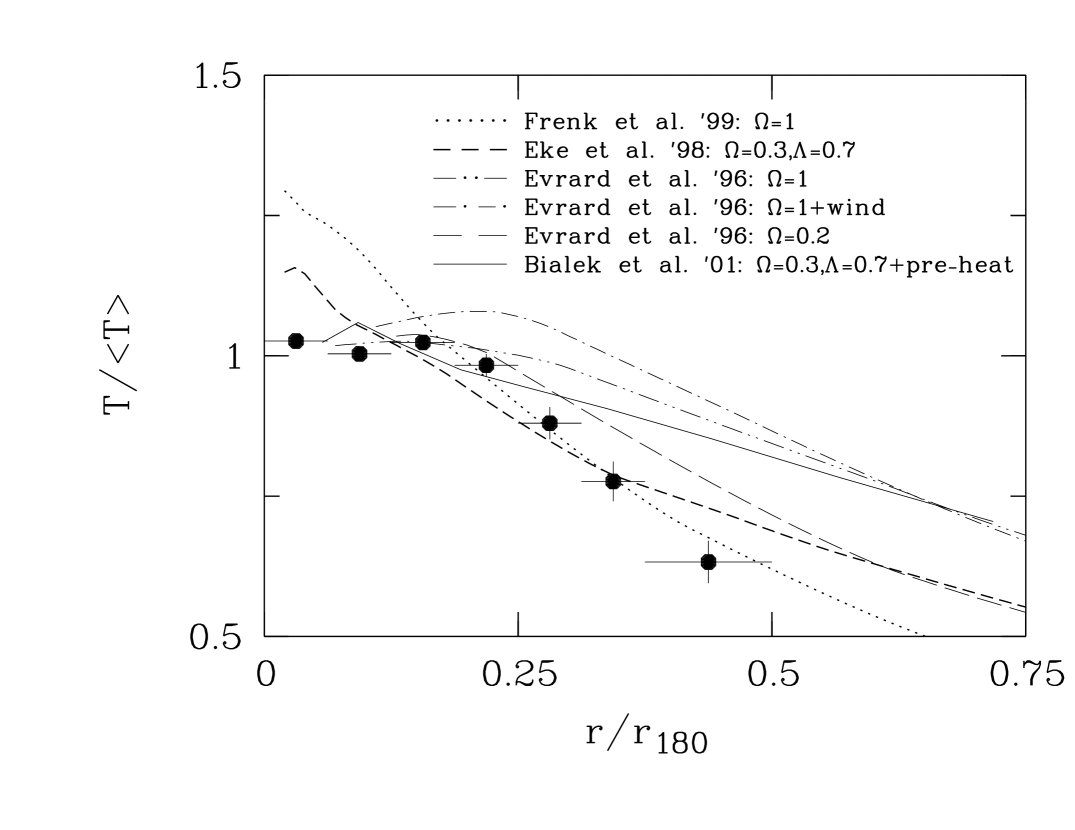
Figure 11: XMM-Newton temperature profiles (open circles) overplotted to our BeppoSAX temperature profiles for A1795 (upper panel) and Coma (lower panel). XMM-Newton data are taken from Arnaud et al. (2001b) for A1795 and from Arnaud et al. (2001a) for Coma; all $90\%$ uncertainties have been converted into $1\sigma$ confidence limits.

Figure 12: Projected emission-weighted temperature profiles from simulations compared to the observed mean temperature profile. Each bin of the observed profile (circles), except for the innermost one, has been computed taking into account all clusters in our sample. In the case of the innermost bin we have averaged data from non-CF clusters only. The simulated projected profiles are all computed for CDM universes and derive from Frenk et al. (1999): $\Omega=1$ (dotted line); Eke et al. (1998): $\Omega=0.3$ $\Lambda=0.7$ (short-dashed line); Bialek et al. (2001): $\Omega=0.3$ $\Lambda=0.7$ with initial entropy-floor S3 (solid line); Evrard et al. (1996): (dot-dot-dashed line) $\Omega=0.1$, $\Omega=1$+wind (dot-dashed line), and $\Omega=0.2$ (long-dashed line).

In this Section we compare our averaged temperature profile to radial temperature profiles derived from hydrodynamic cluster simulations. The mean observed profile shown in Figure 12 (circles) has been computed by including all temperature measurements, except in the innermost bin, where we do not include CF cluster measurements.

The projected emission-weighted temperature profiles derived from hydrodynamic simulations plotted in Figure 12, have been all computed from the three-dimensional profiles following eq. (A2) and (A3) in the Appendix under the hypotheses that the $\alpha$ parameter in eq. (A2) is equal to 0.4 (Ettori 2000), and that the gas density profile is described by a $\beta$-model, $n(r)=n_{o}[1+(r/r_{c})^{2}]^{-{3\over 2}\beta}$, with $r_{c}=0.25$ Mpc and $\beta=2/3$.

In Figure 12 we plot projected temperature profiles computed by Evrard, Metzler & Navarro (1996). These simulations have been designed to explore the effects of galactic winds on the structures of the ICM in a standard Cold Dark Matter (CDM) $\Omega=1$ cosmogony. Here we report three different cases: an $\Omega=1$ without winds, an $\Omega=1$ universe with winds, and an open $\Omega=0.2$ universe without winds. The three-dimensional profiles have been normalized by the authors using the X-ray emission-weighted temperature. As shown in Figure 12 the main characteristic of all these profiles is that in the outer cluster regions they are flatter than the observed profile. These profiles show a pronounced flattening towards the cluster center at a radius similar to that where we observe a flattening in the observed profile, but this effect is probably due to the limited resolution of the simulation.

A simulation with a better resolution was performed by Eke, Navarro & Frenk (1998) for a flat, low-density, $\Lambda$-dominated CDM universe ($\Omega=0.3$, $\Lambda=0.7$). In Figure 12 we plot the projected gas temperature profile computed from the three-dimensional radial profile averaged over 10 cluster simulation at $z=0$ (Eke et al. 1998). The authors have appropriately normalized this profile scaling the individual temperature profiles to the virial temperature of each system. When comparing in Figure 12 their temperature profile with the observed one, we find that the simulated profile is too steep for radii smaller than $\sim 0.2~{}r_{180}$ and that it is too flat for radii larger than $\sim 0.2~{}r_{180}$, failing to reproduce the observed profile at all radii.

Bialek, Evrard & Mohr (2001) have systematically investigated the effects of ICM pre-heating on the basic observed properties of the local cluster population. Bialek et al. have kindly provided us with a projected temperature profile to be compared with our mean temperature profile (see Figure 12). Their profile is the average of twelve cluster simulations performed for a $\Lambda$-CDM cosmology ($\Omega=0.3$, $\Lambda=0.7$) characterized by an initial entropy level of 105.9 keV cm^-2 (entropy level S3 in Bialek et al. 2001), and it is normalized to match our observed core temperature. From Figure 12 we find again that this profile is too flat at large radii to reproduce the observed profile.

The last profile that we have considered is obtained from the Santa Barbara cluster comparison project (Frenk et al. 1999), which simulated the formation of a single X-ray cluster in an $\Omega=1$ universe using twelve nearly-independent codes. As widely discussed in Frenk et al. (1999) the codes show agreement in reproducing the various cluster properties ($\sim 10\%$ agreement for the ICM properties), therefore we will consider in the following the averaged mass-weighted gas temperature profile only (solid line in Figure 17 in Frenk et al. 1999), which was obtained by the authors averaging the data calculated by each code. To normalize the temperature profile we have used the mean temperature computed by fitting with a constant model the profile between $0-1.3$ Mpc, which is the radial range covered on average by the clusters observed in our sample. Using this temperature we have also computed $r_{180}$ as given in Section 4 to normalize the cluster radius. From Figure 12 we firstly note a difference between the Evrard et al. (1996) profile for an $\Omega=1$ universe and the Frenk et al. (1999) profile, which is computed in the same cosmological framework. The Frenk et al. (1999) profile rises rapidly towards the cluster center whereas the Evrard et al. (1996) profile is flatter. This difference is probably due to the smaller resolution of the code used by Evrard et al. (1996), as discussed in the Santa Barbara comparison paper. The difference between our observed temperature profile and that derived by Frenk et al. (1999) is substantial in the inner parts of the clusters where the simulated temperature profile is still rising at the innermost point plotted. In the outer parts of the cluster, both the observed and simulated temperature profile drop in fair agreement.

In general, we can conclude that none of the simulations considered here is able to reproduce the peculiar shape of the observed temperature profile, i.e. the isothermal core in the inner cluster regions followed by a steeply declining temperature profile towards the outer regions. This could suggest that a fundamental ingredient is missing in the construction of the hydrodynamical simulations. This ingredient could be a heat transport mechanism that rapidly brings the ICM within a radius of $\sim 0.2~{}r_{180}$ to the same temperature, indeed the conduction time scale is of the order of a few Gyrs for $r<0.2~{}r_{180}$ (see discussion in Section 5.4.2 of Sarazin 1988). Alternatively, it might be that the merger itself acts as a heat transportation mechanism. Future N-body and theoretical works should be able to reproduce this characteristic feature.

6 Summary

We have performed spatially resolved temperature measurements for a sample of 21 rich and nearby galaxy clusters observed by BeppoSAX. Our sample comprises 10 non-CF and 11 CF clusters. Below we report our main findings.

$\bullet$ The temperature profiles of both CF and non-CF systems are characterized by an isothermal core extending out to $\sim 0.2~{}r_{180}$; beyond this radius both CF and non-CF cluster profiles declines. The temperature drops by a factor of almost 2 from $r\sim 0.2~{}r_{180}$ to $r\sim 0.5~{}r_{180}$.

$\bullet$ Neither the CF nor the non-CF profiles can be modeled by a polytropic temperature profile, the reason being that the radius at which the profiles break is much larger than the core radius characterizing the gas density profiles.

$\bullet$ For $r>0.2~{}r_{180}$ both CF and non-CF temperature profiles can be modeled by a power law, the CF systems have a flatter slope that the non-CF systems. The polytropic indices derived from the power law slopes are respectively $1.46\pm 0.06$ for non-CF systems and $1.20\pm 0.06$ for CF systems. Both values are contained within the isothermal ($\gamma=1$) and the adiabatic ($\gamma=5/3$) case, with the CF systems being closer to the isothermal value and the non-CF systems to the adiabatic value. A possible interpretation is that since for non-CF systems the time from the last major merger is smaller than for the CF systems, heat transport processes will have had more time to act on the CF systems than on the non-CF systems and their temperature profiles will be flatter.

$\bullet$ None of the previously published mean temperature profiles show the characteristic shape, i.e. an isothermal core followed by a rapid decline, that we find. The mean profile found by MFSV98, obtained from ASCA data, shows a smooth decline with no evidence for an isothermal core. The profile found by IB00 from the analysis of 11 BeppoSAX clusters IB00 features a rise of about $10\%$ when going from the center to a radius of $0.3~{}r_{180}$. This profile, as can be seen in Figure 10, is in disagreement with ours. As detailed in Section 3.2, the reason for the difference is most likely the inadequate treatment of the strongback effects in the IB00 analysis of the BeppoSAX data.

$\bullet$ None of the hydrodynamic simulations we have considered reproduces the peculiar shape of the observed temperature profile, i.e. the isothermal core in the inner cluster regions followed by the steep temperature decline in the outer regions. This suggests that a fundamental ingredient is missing in the construction of the hydrodynamical simulations. Future N-body and other theoretical works should be able to reproduce this characteristic feature.

Figure 1: Radial temperature profiles for 3 clusters contained both in our sample and in that of Irwin & Bregman (2000) (i.e. A85, A496 and 2A0335$+$096), as a function of the radius. Filled circles are temperature measurements from Irwin & Bregman (2000), open triangles are derived by us analyzing the data in the same way as in Irwin & Bregman (2000) (see text for details). All error bars are at $1\sigma$ ($68\%$ confidence level); we have converted the $90\%$ errors reported in Figure 2 of Irwin & Bregman (2000) into $68\%$ errors by dividing them by 1.65.

Figure 2: Radial temperature profiles for 3 clusters contained both in our sample and in that of Irwin & Bregman (2000) (i.e. A85, A496 and 2A0335$+$096), as a function of the radius. Filled circles are temperature measurements from Irwin & Bregman (2000), open circles are temperatures derived from our analysis as described in Section 3.

Figure 7: Radial temperature profiles for Coma, Perseus and A1367 as a function of radius in arcminutes derived by analyzing the BeppoSAX data using the corrected (filled circles) and uncorrected (open circles) effective areas.

Figure 8: Break radius in arcminutes, $r^{\prime}_{b}$, computed as described in Section 4.1.6, versus $r^{\prime}_{180}$ in arcminutes. Filled circles are CF clusters, open circles are non-CF clusters.

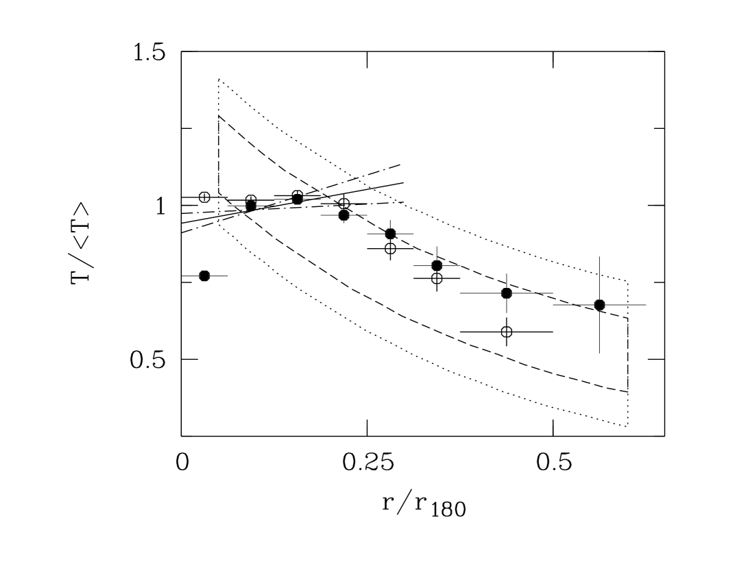
Figure 9: Break radius in units of $r_{180}$ as a function of redshift for all the objects in our sample. Filled circles are CF clusters, open circles are non-CF clusters.

Figure 10: Mean error-weighted temperature profiles for the CF (filled circles) and non-CF (open circles) clusters as a function of the normalized radius. Error bars represent the $1\sigma$ errors. The solid line is the best-fit linear function computed by Irwin & Bregman (2000) with the dot-dashed lines representing the $90\%$ confidence levels of the slope. Also shown is the result in the composite profile found by Markevitch et al. (1998): the dotted box encloses approximately all their temperature profiles and most of the associated error bars, whereas the long-dashed box encloses the scatter of their best-fit values (see Figure 8 in Markevitch et al. 1998).

Table 1: Observation log for the BeppoSAX cluster sample

Target Name	RA(2000)	DEC(2000)	Obs.Date	Obs.Code	Duration
	(degree)	(degree)	yyyy-mm-dd		(ks)
A85	10.3750	-9.3833	1998-07-18	60632001	93
A119	14.0667	-1.2494	2000-07-05	61091002	128
A426 (Perseus)	49.9550	41.5075	1996-09-19	60009001	80
A496	68.4071	-13.2619	1998-03-05	60477001	92
A754	137.3421	-9.6878	2000-05-06	60936001	62
	137.3375	-9.6900	2000-05-17	61091001	123
A1367	176.1208	19.8339	1999-12-21	60832001	97
A1656 (Coma)	194.8950	27.9450	1997-12-28	60126002	68
	194.8950	27.9450	1998-01-19	601260021	24
A1750	202.7188	-1.8408	2000-01-22	60941001	101
A1795	207.2080	26.5917	1997-08-11	604080011	28
	207.2196	26.5922	2000-01-26	60878001	93
A2029	227.7313	5.7439	1998-02-04	60226001	42
A2142	239.5833	27.2333	1997-08-26	60169002	102
A2199	247.1592	39.5514	1997-04-21	60169001	101
A2256	255.9929	78.6419	1998-02-11	60465001	81
	255.9929	78.6419	1999-02-25	60126003	51
A2319	290.3025	43.9494	1997-05-16	60226002	40
A3266	67.8379	-61.4444	1998-03-24	60539002	76
A3376	90.4058	-39.9903	1999-10-17	60936002	110
A3562	203.4100	-31.6700	1999-01-31	60638001	46
A3571	206.8667	-32.8656	2000-02-04	60843002	65
A3627	243.5917	-60.8722	1997-03-01	60180001	34
2A 0335$+$096	54.6458	9.9650	1998-09-11	60675001	105
PKS 0745$-$191	116.8792	-19.2958	1998-10-23	60539001	92

Table 2: Summary of the BeppoSAX MECS radial temperature profiles.

Name	kT	kT	kT	kT	kT	kT	kT	$<$kT$>$	$\chi^{2}$/dof	$z$	$r_{180}$
	0′-2′	2′-4′	4′-6′	6′-8′	8′-12′	12′-16′	16′-20′				Mpc
CF
A85	5.64$\pm$0.13	6.87$\pm$0.19	6.84$\pm$0.27	6.98${}^{+0.68}_{-0.60}$	6.77${}^{+1.31}_{-1.04}$	5.19${}^{+1.10}_{-0.83}$	—	6.83$\pm$0.15	2.35/4	0.0565	3.22
A426 (Perseus)	4.33$\pm$0.04	5.07$\pm$0.04	6.05$\pm$0.08	6.60$\pm$0.12	6.61$\pm$0.17	7.04$\pm$0.19	6.62$\pm$0.21	6.68$\pm$0.08	4.26/3	0.0179	3.19
A496	3.56$\pm$0.07	4.47$\pm$0.10	4.36${}^{+0.14}_{-0.13}$	4.56${}^{+0.23}_{-0.21}$	4.18${}^{+0.44}_{-0.37}$	3.76${}^{+0.55}_{-0.42}$	—	4.42$\pm$0.08	2.55/4	0.0329	2.59
A1795	5.59$\pm$0.10	6.22${}^{+0.16}_{-0.15}$	6.27${}^{+0.25}_{-0.24}$	5.75${}^{+0.36}_{-0.33}$	5.08${}^{+0.85}_{-0.73}$	3.64${}^{+0.80}_{-0.68}$	—	6.10$\pm$0.12	13.0/4	0.0631	3.05
A2029	7.28$\pm$0.22	8.04$\pm$0.35	7.46${}^{+0.49}_{-0.44}$	9.20${}^{+1.52}_{-1.13}$	5.54${}^{+1.24}_{-0.93}$	—	—	7.77$\pm$0.28	5.08/3	0.0766	3.44
A2142	8.26${}^{+0.23}_{-0.22}$	8.88${}^{+0.30}_{-0.29}$	8.79${}^{+0.44}_{-0.43}$	8.45${}^{+0.69}_{-0.66}$	6.96${}^{+1.03}_{-0.83}$	5.96${}^{+1.43}_{-0.92}$	—	8.65$\pm$0.22	6.98/4	0.0899	3.63
A2199	4.25$\pm$0.08	4.54$\pm$0.09	4.59${}^{+0.13}_{-0.12}$	4.80${}^{+0.23}_{-0.19}$	4.42${}^{+0.40}_{-0.38}$	4.60${}^{+0.65}_{-0.50}$	4.32${}^{+0.92}_{-0.67}$	4.62$\pm$0.10	1.01/4	0.0305	2.65
A3562	5.37${}^{+0.42}_{-0.39}$	6.00${}^{+0.50}_{-0.35}$	4.73${}^{+0.46}_{-0.37}$	4.85${}^{+0.80}_{-0.66}$	3.47${}^{+0.89}_{-0.63}$	3.44${}^{+0.72}_{-0.59}$	—	4.82$\pm$0.27	11.5/4	0.0483	2.82
A3571	7.50${}^{+0.27}_{-0.23}$	7.55${}^{+0.26}_{-0.20}$	7.65${}^{+0.32}_{-0.26}$	8.21${}^{+0.52}_{-0.50}$	6.60${}^{+0.62}_{-0.56}$	5.96${}^{+0.80}_{-0.53}$	3.87${}^{+0.61}_{-0.47}$	7.23$\pm$0.17	40.5/6	0.0391	3.32
2A 0335$+$096	2.80$\pm$0.04	3.39$\pm$0.06	3.40${}^{+0.10}_{-0.09}$	3.67${}^{+0.20}_{-0.17}$	3.02${}^{+0.44}_{-0.47}$	2.42${}^{+0.38}_{-0.32}$	—	3.38$\pm$0.08	9.43/3	0.0349	2.27
PKS 0745$-$191	7.14${}^{+0.15}_{-0.14}$	8.52$\pm$0.29	7.58${}^{+0.53}_{-0.42}$	9.07${}^{+1.49}_{-1.15}$	8.02${}^{+3.53}_{-2.10}$	—	—	8.32$\pm$0.25	2.72/3	0.1028	3.56
NON-CF
A119	6.55${}^{+0.48}_{-0.45}$	6.00${}^{+0.31}_{-0.25}$	6.37${}^{+0.34}_{-0.33}$	5.94${}^{+0.40}_{-0.35}$	5.73${}^{+1.02}_{-0.64}$	3.57${}^{+0.37}_{-0.34}$	—	5.66$\pm$0.16	41.1/5	0.0442	2.94
A754	9.45${}^{+0.34}_{-0.30}$	9.36${}^{+0.28}_{-0.25}$	10.40$\pm$0.40	11.63${}^{+0.58}_{-0.54}$	11.66${}^{+0.99}_{-0.83}$	9.08${}^{+0.80}_{-0.69}$	5.04${}^{+0.56}_{-0.50}$	9.42${}^{+0.16}_{-0.17}$	88.1/6	0.0542	3.78
A1367	4.21${}^{+0.43}_{-0.38}$	3.90${}^{+0.28}_{-0.27}$	3.92${}^{+0.23}_{-0.22}$	4.19${}^{+0.27}_{-0.25}$	3.44${}^{+0.35}_{-0.29}$	3.89${}^{+0.28}_{-0.25}$	2.92${}^{+0.22}_{-0.19}$	3.69$\pm$0.10	20.3/6	0.0220	2.37
A1656 (Coma)	9.24${}^{+0.43}_{-0.38}$	10.00$\pm$0.37	9.22$\pm$0.24	9.23$\pm$0.28	8.69${}^{+0.36}_{-0.35}$	9.19${}^{+0.41}_{-0.39}$	8.47${}^{+0.50}_{-0.48}$	9.20$\pm$0.13	8.67/6	0.0222	3.74
A1750	4.74${}^{+0.41}_{-0.30}$	4.25${}^{+0.36}_{-0.33}$	5.31${}^{+0.91}_{-0.73}$	3.95${}^{+0.68}_{-0.51}$	—	—	—	4.46$\pm$0.24	2.23/3	0.0852	2.52
A2256	7.20${}^{+0.27}_{-0.26}$	7.15${}^{+0.20}_{-0.19}$	7.23${}^{+0.23}_{-0.22}$	6.93${}^{+0.33}_{-0.32}$	5.53${}^{+0.48}_{-0.43}$	4.70${}^{+0.60}_{-0.53}$	—	6.97$\pm$0.12	25.8/5	0.0570	3.26
A2319	9.67${}^{+0.66}_{-0.48}$	9.65${}^{+0.55}_{-0.43}$	10.15${}^{+1.11}_{-0.97}$	9.76${}^{+1.80}_{-1.21}$	12.46${}^{+2.27}_{-1.76}$	10.40${}^{+2.21}_{-1.67}$	—	9.82$\pm$${}^{+0.37}_{-0.38}$	1.66/5	0.0560	3.86
A3266	9.22${}^{+0.65}_{-0.53}$	9.34${}^{+0.53}_{-0.42}$	9.47${}^{+0.67}_{-0.50}$	8.47${}^{+0.72}_{-0.68}$	8.30${}^{+1.11}_{-0.98}$	7.44${}^{+1.80}_{-1.38}$	5.11${}^{+1.92}_{-1.23}$	8.97${}^{+0.29}_{-0.30}$	6.82/6	0.0550	3.69
A3376	4.23${}^{+0.36}_{-0.32}$	3.82${}^{+0.21}_{-0.18}$	4.27${}^{+0.27}_{-0.25}$	3.96${}^{+0.33}_{-0.30}$	3.48${}^{+0.60}_{-0.46}$	—	—	3.99$\pm$0.13	2.92/4	0.0455	2.46
A3627	6.29${}^{+0.64}_{-0.55}$	7.28${}^{+0.53}_{-0.44}$	6.12${}^{+0.36}_{-0.30}$	7.10${}^{+0.50}_{-0.45}$	5.59${}^{+0.46}_{-0.41}$	6.10${}^{+0.51}_{-0.38}$	5.76${}^{+0.53}_{-0.44}$	6.28$\pm$0.18	9.91/6	0.0163	3.09

Table 3: Best-fits parameters and $\chi^{2}$ values for phenomenological models.

Model	${T\over<T>}=c$	${T\over<T>}=a+b({r\over r_{180}})$	${T\over<T>}=f(t_{b},x_{b},m)\tablenotemark{a}$
Sample	$~{}~{}~{}~{}c$   $~{}~{}~{}~{}~{}~{}~{}~{}~{}\chi^{2}$/dof	$a$             $~{}~{}~{}b$       $~{}~{}~{}~{}\chi^{2}$/dof	$t_{b}$        $~{}~{}~{}~{}~{}x_{b}$         $~{}~{}~{}m$       $~{}\chi^{2}$/dof
non-CF	$1.00\pm 0.01$   $231.3/61$	$1.08\pm 0.01$  $-0.77\pm 0.08$  $141.4/60$	$1.02\pm 0.01$   $0.23\pm 0.01$  $-2.56^{+0.24}_{-0.25}$  $87.9/59$
CF	$1.00\pm 0.01$   $82.9/50$	$1.07\pm 0.01$  $-0.55\pm 0.10$    $54.2/49$	$1.01\pm 0.01$   $0.16\pm 0.03$  $-1.13^{+0.19}_{-0.28}$  $36.2/48$
all	$1.00\pm 0.01$   $314.3/112$	$1.08\pm 0.01$  $-0.68\pm 0.06$  $199.8/111$	$1.02\pm 0.01$   $0.20\pm 0.03$  $-1.79^{+0.29}_{-0.49}$  $137.4/110$

Table 4: Best-fits parameters and $\chi^{2}$ values for polytropic models.

Model	${T\tablenotemark{a}\over<T>}=f(t_{o},\gamma,r_{c})$	${T\tablenotemark{b}\over<T>}=f(t_{o},\gamma)$
Sample	$~{}~{}~{}~{}~{}\gamma^{\tablenotemark{c}}$       $~{}~{}~{}r_{c}$(Mpc)   $~{}~{}~{}\chi^{2}$/dof	$~{}~{}~{}~{}\gamma$        $~{}~{}~{}~{}\chi^{2}$/dof
non-CF	$1.67^{+*}_{-0.08}$   $1.49^{+0.06}_{-0.13}$   $120.7/59$	$1.09\pm 0.01$    $159.7/60$
CF	$1.67^{+*}_{-0.23}$   $1.73^{+0.19}_{-0.38}$   $45.49/48$	$1.06\pm 0.01$    $61.76/49$
all	$1.67^{+*}_{-0.07}$   $1.54^{+0.08}_{-0.11}$   $170.2/110$	$1.07\pm 0.01$    $225.9/111$

Table 5: Best-fits parameters and $\chi^{2}$ values for polytropic models applied to radii larger than $0.2~{}r_{180}$.

Model	${T\tablenotemark{a}\over<T>}=t_{o}({x\over x_{o}})^{-\mu}$
Sample	$~{}~{}~{}~{}~{}~{}~{}\mu$       $~{}~{}~{}T(r=0.3r_{c})/<T>$  $~{}~{}~{}\chi^{2}$/dof
non-CF	$0.92\pm 0.12$           $0.81\pm 0.02$          $29.57/16$
CF	$0.39\pm 0.11$           $0.84\pm 0.03$          $12.45/23$
all	$0.64\pm 0.08$           $0.82\pm 0.02$          $52.65/39$

Appendix A Appendix

We assume that at large radii the three-dimensional gas temperature and density profiles $T(r)$ and $n(r)$ can be described by power-laws of the form:

$$T(r)=T_{o}(r/r_{o})^{-\mu}~{}~{}{\rm and}~{}~{}n(r)=n_{o}(r/r_{o})^{-\nu}.$$

We approximate the emissivity $\epsilon(r)$ in a given spectral band with the expression given in Ettori (2000),

$$\epsilon(r)=n^{2}(r)\lambda T^{\alpha},$$

where $\lambda$ is a numerical constant and values for $\alpha$ may be found in Table 1 of Ettori (2000). The projected emission weighted temperature profile $T(b)$ and surface brightness profile $S(b)$, where $b$ is the projected radius, are defined as:

$$T(b)\equiv{\int_{0}^{\infty}\epsilon(r)T(r)dl\over\int_{0}^{\infty}\epsilon(r)dl}~{}~{}~{}{\rm and}~{}~{}~{}S(b)\equiv 2\int_{0}^{\infty}\epsilon(r)dl,$$

where the integration is along the line of sight, $l$, and the relation $r^{2}=b^{2}+l^{2}$ is valid. By substituting equations (A1) and (A2) in equation (A3) and by making use of the integration rule:

$$\int_{0}^{\infty}(l^{2}+b^{2})^{-z}dl={\sqrt{\pi}\over 2}{\Gamma(z-1/2)\over\Gamma(z)}b^{1-2z},$$

where $\Gamma$ is the gamma function, we find that the projected temperature and surface brightness profiles can be expressed as power-laws of the form:

$$T(b)=T^{\prime}_{o}(b/r_{o})^{-\mu^{\prime}}~{}~{}{\rm and}~{}~{}S(r)=S_{o}(b/r_{o})^{-\nu^{\prime}},$$

where:

$$~{}~{}\mu^{\prime}=\mu~{}~{}~{}~{}{\rm and}~{}~{}~{}T^{\prime}_{o}={\Gamma[1/2(2\nu+(\alpha+1)\mu)-1/2]~{}~{}\Gamma[1/2(2\nu+\alpha\mu)]\over\Gamma[1/2(2\nu+(\alpha+1)\mu)]~{}~{}\Gamma[1/2(2\nu+\alpha\mu)-1/2]}~{}~{}T_{o},$$

$$~{}~{}\nu^{\prime}=2\nu+\alpha\mu-1~{}~{}~{}{\rm and}~{}~{}~{}S_{o}=2\lambda n_{o}^{2}T_{o}^{\alpha}r_{o}~{}{\Gamma[1/2(2\nu+\alpha\mu)-1/2]\over\Gamma[1/2(2\nu+\alpha\mu)]}.$$

The polytropic index $\gamma$, for a gas described by equation (A1) is $\gamma=\mu/\nu+1$. Using equations (A6) and (A7) it can be expressed directly in terms of the observables $\mu^{\prime}$ and $\nu^{\prime}$:

$$\gamma~{}=~{}\Big{(}{\nu^{\prime}\over 2}+{1\over 2}-\alpha\mu^{\prime}\Big{)}\mu^{\prime}+1.$$

Similar formulae have been derived by Ettori (2000). In that paper the surface brightness profile was described by a $\beta$-model and a polytropic relation was assumed between the gas density $n$ and temperature $T$. Here we do not assume a polytropic relation to hold at all radii (our data shows that this is not the case) and we limit ourselves to the outer regions where a power-law behavior holds for both the surface brightness profile and the projected temperature profile. The aim of this Appendix is to show that under the sole assumption that the gas density $n(r)$ and temperature $T(r)$ are described by power-laws, $n(r)$, $T(r)$ and the polytropic index, $\gamma$, can be derived analytically from the parameters obtained by fitting the surface brightness profile and the projected temperature profile with power-laws.

References

- (1) Allen, S. W., Fabian, A. C., Johnstone, R. M., Arnaud, K. A., Nulsen, P. E. J. 2001, MNRAS, 322, 589
- (2) Arnaud, M. et al. 2001a, A&A, 365, L67
- (3) Arnaud, M., Neumann, D. M., Aghanim, N., Gastaud, R., Majerowicz, S. & Hughes, J. P. 2001b, A&A, 365, L80
- (4) Bardelli, S., De Grandi, S., Ettori, S., Molendi, S., Zucca, E. & Colafrancesco, S. 2001, A&A, in press
- (5) Bialek, J. J., Evrard, E. E. & Mohr, J. J. 2001, ApJ, 555, 597
- (6) M. Bliton, M., Rizza, E., Burns, J. O., Owen, F. N. & Ledlow, M. J. 1998, MNRAS, 301, 609
- (7) Boella, G., et al. 1997a, A&AS, 122, 327
- (8) Boella, G., Butler, R. C., Perola, G. C., Piro, L., Scarsi, L., & Bleeker, J. A. M. 1997b, A&AS, 122, 299
- (9) Briel, U. G. & Henry, J. P. 1994, Nat, 372, 439
- (10) Briel, U. G. & Henry, J. P. 1996, ApJ, 472, 131
- (11) D’Acri, F., De Grandi, S., & Molendi S. 1998, Nuclear Physics, 69/1-3, 581 (astro-ph/9802070)
- (12) David, L. P. et al. 2000 (astro-ph/0010224)
- (13) Davis, D. S. & White, R. E. III 1998, ApJ, 492, 57
- (14) De Grandi, S. & Molendi, S. 2001, ApJ, 551, 153
- (15) De Grandi, S. & Molendi, S. 1999, ApJ, 527, L25
- (16) De Grandi, S. & Molendi, S. 1999, A&A, 351, L45
- (17) Dickey, J. M. & Lockman, F. J. 1990, ARA&A, 28, 215
- (18) Dupke, R. A. & Bregman, J. N. 2001, ApJ, 547, 705
- (19) Eke, V. R., Navarro, J. F. & Frenk, C. S. 1998, ApJ, 503 569
- (20) Ettori, S. 2000, MNRAS, 311, 313
- (21) Ettori, S., Bardelli, S., De Grandi, S., Molendi, S., Zamorani, G., Zucca, E. 2000, MNRAS, 318, 239
- (22) Ettori, S. & Fabian, A. C. 1999, MNRAS, 305, 834
- (23) Evrard, A. E., Metzler, C. A. & Navarro, J. F. 1996, ApJ, 469, 494
- (24) Ezawa, H., Yamasaki, N. Y., Ohashi, T., Fukazawa, Y., Hirayama, M., Honda, H., Kamae, T., Kikuchi, K., Shibata, R. 2001, PASJ, 53, 595
- (25) Fabian, A. C., Hu, E. M., Cowie, L. L., Grindlay, J. 1981, ApJ, 248, 47
- (26) Finoguenov, A., Arnaud, M. & David, L. P. 2001, ApJ, 555, in press
- (27) Finoguenov, A., Reiprich, T. H. & Böhringer, H. 2001, A&A, 368, 749
- (28) Frenk, C. S., et al. 1999, ApJ, 525, 554
- (29) Henriksen, M. J. & Markevitch, M. L. 1996, ApJ, 466, L79
- (30) Henry, J. P. 1997, ApJ, 489, L1
- (31) Irwin,J. A., Bregman, J. N. & Evrard, A. E. 1999, ApJ, 519, 518
- (32) Irwin, J. A. & Bregman, J. N. 2000, ApJ, 538, 543 (IB00)
- (33) Knopp, G. P., Henry, J. P. & Briel, U. G. 1996, ApJ, 472, 125
- (34) Lloyd-Davies, E. J., Ponman, T. J. & Cannon, D. B. 2000, MNRAS, 315, 689
- (35) Maccacaro, T., Gioia, I. M., Wolter, A., Zamorani, G., Stocke, J.T. 1988, ApJ, 326, 680
- (36) Markevitch, M., Forman, W. R., Sarazin, C. L. & Vikhlinin, A. 1998, ApJ, 503, 77 (MFSV98)
- (37) Markevitch, M., Vikhlinin, A., Forman, W. R. & Sarazin, C. L. 1999, ApJ, 527, 545
- (38) Mohr, J. J., Reese, E. D., Ellingson, E., Lewis, A. D., Evrard, A. E. 2000, ApJ, 544, 109
- (39) Mohr, J. J., Mathiensen, B. & Evrard, A. E. 1999, ApJ, 517, 627
- (40) Molendi, S. & De Grandi., S. 1999, A&A, 351, L41
- (41) Molendi, S., De Grandi., S., Fusco-Femiano, R., Colafrancesco, S., Fiore, F., Nesci, R. & Tamburelli, F. 1999, ApJ, 525, L73
- (42) Molendi, S., De Grandi, S. & Fusco-Femiano, R. 2000, ApJ, 534, L43
- (43) Molendi, S. & Pizzolato, F. 2001, ApJ, 560, 194
- (44) Nevalainen, J., Markevitch, M. & Forman, W. 2000, ApJ, 532, 649
- (45) Nevalainen, J., Kaastra, J., Parmar, A. N., Markevitch, M., Oosterbroek, T., Colafrancesco, S., Mazzotta, P. 2001, A&A, 369, 459
- (46) Peres, C. B., Fabian, A. C., Edge, A. C., Allen, S. W., Johnstone, R. M., & White, D. A. 1998, MNRAS, 298, 416
- (47) Sarazin, C. L. 1988, “X-Ray emission from clusters of galaxies”, Cambridge Astrophysics Series, Cambridge: Cambridge University Press.
- (48) Sanders, J. S., Fabian, A. C. & Allen, S. W. 2000, MNRAS, 318, 733
- (49) Tamura, T. et al. 2001, A&A, 365, L87
- (50) Vecchi, A., Molendi, S., Guainazzi, M., Fiore, F., Parmar, A. N. 1999, A&A, 349, L73
- (51) Verde, L., Kamionkowski, M., Mohr, J. J. & Benson, A. J. 2001, MNRAS, 321, L7
- (52) Voit, G. M. 2000, ApJ, 543, 113
- (53) White, S. D. M., Navarro, J. F., Evrard, A. E. & Frenk, C. S. 1993, Nat, 366, 429
- (54) White, D. A. 2000, MNRAS, 312, 663
- (55) Zabludoff, A. I. & Zaritsky, D. 1995, 447, L21