On the Nature of the EIS Candidate Clusters: Confirmation of $z\lesssim 0.6$ candidates

We use publicly available $V$-band imaging data from the wide-angle surveys conducted by the ESO Imaging Survey project (EIS) to further investigate the nature of the EIS galaxy cluster candidates. These were originally identified by applying a matched-filter algorithm which used positional and photometric data of the galaxy sample extracted from the $I$-band survey images. In this paper, we apply the same technique to the galaxy sample extracted from $V$-band data and compare the new cluster detections with the original ones. We find that $\sim 75\%$ of the low-redshift cluster candidates ($z\lesssim 0.6$) are detected in both passbands and their estimated redshifts show good agreement with the scatter in the redshift differences being consistent with the estimated errors of the method. For the “robust” $I$-band detections the matching frequency approaches $\sim 85\%$. We also use the available $(V-I)$ color to search for the red sequence of early-type galaxies observed in rich clusters over a broad range of redshifts. This is done by searching for a simultaneous overdensity in the three-dimensional color-projected distance space. We find significant overdensities for $\sim 75\%$ of the “robust” candidates with $z_{I}\lesssim 0.6$. We find good agreement between the characteristic color associated to the detected ”red sequence” and that predicted by passive evolution galaxy models for ellipticals at the redshift estimated by the matched-filter. The results presented in this paper show the usefulness of color data, even of two-band data, to both tentatively confirm cluster candidates and to select possible cluster members for spectroscopic observations. Based on the present results, we estimate that $\sim 150$ EIS clusters with $z_{I}\lesssim 0.6$ are real, making it one of the largest samples of galaxy clusters in this redshift range currently available in the southern hemisphere.

1 Introduction

Clusters of galaxies are prime targets in observational cosmology for several reasons among which: they are the largest gravitationally bound structures observed in the universe and as such are useful tracers of the large-scale structure; their abundance as a function of redshift can set strong constraints on the cosmological parameters; studies of the properties of cluster galaxies can provide insight on their star-formation and merging history and set valuable constraints to galaxy formation and evolution models. However, such studies are only possible using statistically representative samples of clusters spanning a large range of redshifts. Unfortunately, such samples are currently not available, with most of the existing cluster catalogs being either limited in number or redshift coverage. In recent years, several attempts have been made to conduct systematic searches for more distant systems both in optical/infrared and X-ray utilizing a large variety of detection techniques (e.g. Gunn et al. 1986; Lidman & Peterson 1996; Lumsden et al. 1992; Postman et al. 1996; Zaritsky et al. 1997; Gonzalez et al. 2001; Gladders & Yee 2000). Other promising methods include the use of mass reconstruction maps built from weak lensing signals and the Sunyaev-Zeld’ovich effect to conduct blind cluster searches over wide areas.

While the number of candidates has significantly increased, especially from optical/infrared searches, the number of confirmed and well-studied cases with $z\sim 1$ remains relatively small (e.g. Postman et al. 2001). Therefore, the present samples fall far short of what is desirable for: exploring the relationship between systems selected using different detection algorithms, a more complete characterization of cluster properties and a better understanding of the evolution of clusters and their galaxy population. The major obstacles for enlarging the sample of well-studied cluster galaxies have been a combination of several factors which include the reliability of cluster candidates, interloper contamination and instrumental limitations. The reliability issue has in general favored follow-ups of X-ray selected samples, which are currently small and unlikely to grow significantly in the near future. Therefore, to immediately benefit from the available large aperture telescopes and multi-object spectrographs for galaxy cluster research, for the time being one must rely on optical/infrared surveys such as those being carried out by the ESO Imaging Survey (EIS) project. Using the original $I$-band survey data (Nonino et al. 1999; Prandoni et al. 1999; Benoist et al. 1999) a catalog of cluster candidates was compiled (Olsen et al. 1999a, b; Scodeggio et al. 1999) comprising $\gtrsim 300$ candidates in the redshift range $0.2\leq z\leq 1.3$ within an area of $\sim 15$ square degrees, until recently the largest publicly available sample of its kind in the southern hemisphere. However, candidate clusters based on a single passband are normally viewed with skepticism because of the known problems caused by projection effects. In order to address this concern, in the present paper we use the publicly available $V$-band data to demonstrate that by using color information one can provide independent supporting evidence of the reality of a large fraction of the candidate clusters.

We use the available $V$ data in two complementary ways. First, we extend the analysis carried out by Olsen et al. (1999b) and treat the data from the $V$-survey as an independent data set to which we apply the matched-filter algorithm and test the reproducibility of the detections. The $V$-detections are then cross-compared to those obtained from the analysis of the $I$-band data. Second, we use the $(V-I)$ color to search for a simultaneous spatial and color concentration at the location of the $I$ detections. Such concentrations are interpreted as being associated with the red sequence observed in rich clusters over a broad range of redshifts (e.g. Aragón-Salamanca et al. 1993; Stanford et al. 1998; Lubin 1996). This red sequence is interpreted as being an indication that rich clusters contain a core population of passively evolving elliptical galaxies which are old and coeval. This method is similar to that described by Gladders & Yee (2000) in the so-called red sequence cluster survey.

The $V$-band data restricts the analysis primarily to cluster candidates with $z\lesssim 0.6$ since at larger redshifts ellipticals dropout from the sample as the 4000Å break moves past the $V$-band. However, the analysis presented here illustrates the methodology that will be employed in forthcoming papers to investigate high-redshift candidates using the multi-color optical/infrared ($R$ and $JK_{s}$) imaging data assembled for a large number of EIS candidates with $z\geq 0.5$ ($\sim 110$ and $\sim 40$). These data will also be combined with the results of ongoing spectroscopic observations being conducted at the 3.6m telescope at La Silla (e.g. Ramella et al. 2000) and at the VLT of color-selected systems in different redshift intervals. Preliminary results based on an admittedly small sample suggest that a significant fraction of these color-selected systems are confirmed spectroscopically.

This paper is organized as follows. Sect. 2 briefly describes the data used in the present analysis. Sect. 3 presents the results obtained from the comparison of matched-filter detections in $V$ and $I$, from which a first estimate of the confirmation rate is derived. Sect. 4 describes the methodology employed to detect early-type cluster members and to measure the typical color associated to these objects. This information is used to obtain independent estimates of the expected confirmation rate and the redshifts assigned to them. A discussion of the results is presented in Sect. 5. A brief summary of our results is given in Sect. 6.

2 The Data

In the present analysis we use the catalog of EIS candidate clusters compiled by Olsen et al. (1999a, b) and Scodeggio et al. (1999) comprising $\gtrsim 300$ candidates over four patches of the sky covered by the EIS-WIDE $I$-band survey conducted at the NTT. The candidates were identified from the galaxy distribution extracted from these images and presented in Nonino et al. (1999), Prandoni et al. (1999) and Benoist et al. (1999).

In this paper the $I$-data are complemented with those taken in $V$. The $V$-data consists of two sets of images. One taken at the NTT with EMMI, as part of the original EIS-WIDE survey which covered two square degrees (Patches A and B). The other consists of images taken at the MPG/ESO 2.2 m telescope with ESO’s Wide-Field Imager (WFI) as part of the so-called Pilot Survey. The latter set covers a total area of 12 square degrees in $V$-band, out of which 6 square degrees are publicly available. Galaxy catalogs have been extracted from these $V$-images and associated with those in $I$ to produce $(V-I)$ color catalogs utilized below, covering a total area of 8 square degrees, or about half the area of the $I$-survey. Within this area there are 168 $I$-band cluster candidates, corresponding to 55% of the entire EIS candidate sample.

Fig. 1 compares the galaxy counts obtained from the $V$-band catalogs extracted from the images taken using different telescope/detector setups. Even though reaching different limiting magnitudes, the counts are consistent with each other and in good agreement with those of other authors (Arnouts et al. 1995). This demonstrates the uniformity of the galaxy catalogs, which are not distinguished in the analysis below. The $5\sigma$-limiting magnitudes are estimated to be $V\sim 24$ and $V\sim 24.6$ (da Costa et al. 2000) for the EIS-WIDE (patches A and B) and Pilot Survey data (patch D), respectively. Therefore, in the analysis presented below we only consider galaxies brighter than $V=24$.

Figure 1: Galaxy number counts derived from the $V$-band images obtained for EIS Patches A (dashed-dotted line) and B (dashed line) and the Pilot Survey (Patch D, dotted line). For comparison the counts of Arnouts et al. (1995) (open circles) are also shown.

3 Searching for clusters in $V$-band

3.1 Matched-filter Detections

The EIS cluster search was using the matched-filter algorithm originally proposed by Postman et al. (1996) and used to build the Palomar Distant Cluster Survey (PDCS). This method uses a filter built from the luminosity function and radial profile of nearby clusters. At each position of the survey area the probability of the presence of a cluster matching the filter is computed. By fine-tuning the filter to match the apparent magnitudes and extent of the cluster at a series of redshifts ($0.2\leq z\leq 1.3$) a likelihood curve is constructed. The cluster candidate is then assigned the redshift for which the maximum likelihood is found.

In contrast to the PDCS the EIS cluster catalog was built exclusively from matched-filter detections in the $I$-band for which two sets of images, contiguously covering the regions of interest, were available. These sets were treated separately to construct two galaxy catalogs which were called “odd” and “even” catalogs, to indicate the image mosaic from which they were extracted. The matched-filter algorithm was run on each catalog and the resulting cluster detections were compared. The detections were considered to be: “robust” if they were detected at $4\sigma$ in one or both catalogs, or if they were detected at the $3\sigma$-level in both the “even” and “odd” catalogs, and “poor” if they were detected at the $3\sigma$-level in only one of the catalogs. These definitions were introduced by Olsen et al. (1999a) (see also Scodeggio et al. 1999) and are used below.

The $V$ images available represent another sampling of the galaxy distribution in the region and as such can be used to define another set of cluster candidates. In applying the matched-filter procedure to the galaxy catalogs extracted from the $V$-band images, we use the same cluster model as in $I$. This model assumes a Schechter luminosity function and a radial distribution of galaxies given by a truncated Hubble profile (for more details see Olsen et al. 1999a). Following Postman et al. (1996) we adopt the Schechter parameters $M^{*}_{V}=-21.02$ and a faint end slope of $\alpha=-1.1$, valid for local clusters. For the radial profile we adopt a core radius of $r_{\mathrm{c}}=100h^{-1}\mathrm{kpc}$ and a cut-off radius of $r_{\mathrm{co}}=1h^{-1}\mathrm{Mpc}$. We use a cosmological model with $H_{0}=75\mathrm{km/s/Mpc}$, $\Omega_{0}=1.0$.

In the discussion presented below it is important to have a rough idea of the redshift limit for cluster detection in each of the passbands. This can be obtained from the limiting magnitudes of the input galaxy catalogs ($I_{\mathrm{lim}}\sim 23$ and $V_{\mathrm{lim}}\sim 24$, Vega system), by assuming that the cluster population is formed predominantly by early-type galaxies, and by assuming a particular model for the evolution of the stellar population. The maximum contrast of a cluster over the field population occurs in the range of magnitudes $m^{*}\pm 1\mathrm{mag}$, where $m^{*}$ is the apparent Schechter magnitude of the cluster. Therefore, the limiting redshift corresponds approximately to that for which $m^{*}+1$ is comparable to the limiting magnitude of the galaxy catalog. Assuming a no-evolution model this would, for the data considered here, imply a redshift limit of $z\sim 0.6$ and $z\sim 1.1$ for the $V$- and $I$-candidates, respectively. If one instead assumes a passive-evolution model the redshift limits would become slightly larger. As it will be seen below, $z\sim 0.6$ as determined for the $V$-band is indeed the practical limit of the present analysis.

Figure 2: The matching rate as function of redshift for the “robust” (left column) and “poor” (right column) candidates as explained in the text. The upper panel shows the redshift distribution for all the candidates (dashed histogram) and those with counterparts in the $V$-band (filled histogram). The lower panel shows the respective matching frequency as function of redshift which is interpreted as an estimate of the confirmation rate of the original $I$-detections.

3.2 Comparison between $V$- and $I$-detections

The cluster candidates identified by applying the matched-filter algorithm to the galaxy catalogs extracted from the $V$ images are compared to the $I$-band candidates. Below we only consider those which match $I$-candidates, even though there are also $V$-candidates without corresponding $I$-detections ($\sim 40$, which will be discussed elsewhere). Detections in the different passbands are matched by considering only positional coincidence. For this we require the angular separation to correspond to a projected separation of less than $0.5h^{-1}\mathrm{Mpc}$ at the redshift estimated for the $I$-candidate ($z_{I}$), regardless of the matched-filter redshift estimate, $z_{V}$, based on the $V$ catalogs. In the following we investigate the frequency of matches and compare the $V$- and $I$-estimated redshifts.

Fig. 2 summarizes the results of the cross-comparison between $V$- and $I$-candidates. The top panels show the redshift distribution of the matched candidates compared with the redshift distribution of the sub-sample of EIS $I$-candidates located within the area covered by $V$. The left panels refer to “robust” candidates (90 candidates) and the right to the “poor” ones (78 candidates). The overall matching rate is 61% (102 out of 168 $I$-band candidates), and varies with redshift as shown in the lower panels of Fig. 2.

From Fig. 2 one sees that for $z_{I}\leq 0.6$ most clusters are detected in both passbands. In this redshift interval the matching rate (hereafter interpreted as an estimate of the confirmation rate) for the whole sample is $\sim 75\%$ (88 out of 118). Additionally restricting the sample to “robust” candidates, the confirmation rate is higher, reaching $\sim 82\%$ (69 out of 81). It is also interesting to note that about 50% of the “poor” candidates in this redshift range are associated with $V$-detections, showing an above average rate at $z_{I}=0.3$. This could be due to low-redshift poor clusters detected at a low significance level in a single-passband.

At larger redshifts ($z_{I}\geq 0.7$) only 14 ($\sim 26\%$) of the 54 $I$-band cluster candidates are matched by a $V$-detection. This lower confirmation rate is not surprising considering that for systems with $z\gtrsim 0.6$ the 4000Å break lies redwards of the $V$-band. Note, however, that we find matching $V$-detections over a broad range of redshifts including some very high-redshift systems ($z_{I}\gtrsim 1$), especially in the ”poor” sample. In order to investigate the nature of these matches the 14 cases of clusters with $z_{I}>0.6$ and with matched $V$ detections were visually inspected. In five cases ($z_{I}=0.7,0.7,0.9,1.1,1.3$) the $V$-detection is clearly associated with a foreground concentration unrelated to the $I$-band cluster candidate, even though the $I$-band image does appear to include a cluster candidate. In one case ($z_{I}=1.3$) the $V$-image contains a satellite track which leads to spurious galaxy detections forming an artificial concentration of objects in the $V$ catalog. For the remaining eight cases the $V$-band images do show concentrations of galaxies consistent with those seen in $I$. These eight candidates - four robust and four poor $I$-detections - have redshifts in the range 0.7-1.1. As mentioned above, while early-type galaxies are not expected to be detected in this redshift range, the cluster detection based on the matched filter technique takes into account the entire galaxy population. Therefore, this makes this method less sensitive than others (see below) to the fading in the $V$-band of the early-type galaxies. One should also keep in mind the large uncertainties in the redshift estimates at high redshift, which could lead to the matching $VI$-detections with large differences in redshift estimates. However, as shown below this does not seem to be the case. Of course, there is still the possibility of the superpositions of clusters at different redshifts with $I$ detecting a distant richer system, while $V$ detecting a foreground one. Deciding among these possibilities will have to await the results of spectroscopic observations. Note that a comparable fraction of $VI$ detections in the redshift interval being considered was found by Postman et al. (1996) (see also Lubin 1996).

Figure 3: The distribution of differences of redshifts estimated from the $V$ and $I$ matched-filter identifications for the entire sample (dashed line) and the “robust” candidates (solid line).

3.3 Redshift Comparison

Besides confirming $I$-candidates, the $V$-detections can also be used to assess the reliability of the original cluster redshift estimates based on the application of the matched-filter algorithm to the $I$-band galaxy catalog. Fig. 3 shows the distribution of redshift differences estimated by the matched-filter algorithm for associated $V$- and $I$-detections. The figure shows this distribution for the whole sample, considering matches over the entire redshift range, but eliminating the six spurious matches discussed in the previous section. Also shown is the distribution of redshift differences for the sample of “robust” candidates. Taking the sample as a whole, we find a mean difference of $\langle z_{V}-z_{I}\rangle=-0.03$ and a scatter of $0.12$. For the “robust” candidates the mean difference is significantly smaller $\langle z_{V}-z_{I}\rangle=-0.003$ with a scatter of $0.11$. Interestingly, all the eight cases with matched $VI$ detections and redshifts $z_{I}>$0.6, discussed in the previous section, have consistent redshifts within the estimated errors, giving further credence to their confirmation. Note that two of the “robust” cases are outliers - one with $(z_{V}-z_{I})=0.5$, $z_{V}=0.7$ and $z_{I}=0.2$; another with $(z_{V}-z_{I})=-0.4$, $z_{V}=0.2$ and $z_{I}=0.6$. To investigate these cases we visually inspected the images and the “even” and “odd” detection lists (see Sect. 3.1). From this inspection we conclude that: in the first case the cluster seems real in both bands. However, the original $I$-detection had two different redshifts in the “even” ($z_{I}=0.4$) and “odd” ($z_{I}=0.2$) catalogs. The latter was included in the EIS cluster candidate catalog, because it had a higher significance. Clearly, for this cluster $z_{I}$ is uncertain, but there is little doubt about the reality of the cluster. In the second case the redshift discrepancy is probably due to the superposition of a low redshift system detected in $V$ and a more distant cluster detected in $I$. Finally, we emphasize that the above results also demonstrate the reliability of the redshift estimates and can be used for selecting sub-samples in different redshift intervals, if an error of about 0.15 is properly taken into account.

4 Searching for cluster early-types

Confirmation of candidate clusters by matching $V$ and $I$ relies only on the fact that the $V$ images and the derived galaxy catalogs may suffer different effects than those in $I$-band. Thus, the reproducibility of the results obtained from data in different passbands serves to corroborate the original findings, thereby increasing the significance of the detections. This test, however, relies on the same underlying assumptions of the matched-filter method - clusters are nearly spherical, have the same projected density profile and are characterized by a Schechter luminosity function, similar to the one observed in local clusters.

An alternative way of searching or checking the reality of clusters is to use the additional information provided by the $(V-I)$ color. One way is to search, at the location of the $I$ detections, for early-type galaxies which are known to form a tight color-magnitude relation and to populate the central regions of galaxy clusters. Another is to conduct blind searches for clustering of early-type galaxies with colors consistent with their being at different redshift intervals. These methods make no assumption about the global properties of clusters but have to rely on galaxy evolution models. These color-based methods are complementary to the matched-filter approach. In addition, splitting galaxy catalogs in color intervals leads to an increase in the contrast between the cluster and the background. This enhanced contrast can be particularly important for the confirmation of poor cluster candidates. Consistency between the two approaches, for reasonable models of galaxy evolution, can thus lend further support to the reality of a cluster candidate. Additionally, an important advantage of color-based methods is that they provide a sample of candidate early-type cluster members which can be used for follow-up spectroscopic observations.

4.1 Color-slicing procedure

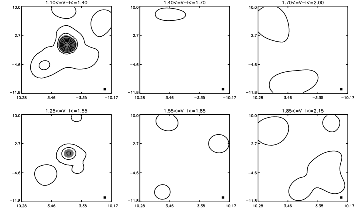
Figure 4: Six density maps for one cluster candidate. The upper and lower row each correspond to the first three maps of each of the subsets of seven density maps. The remaining eight slices do not contain relevant information in this particular case. The two sets are shifted by half the width of a color slice to make sure that a cluster is not split between two slices, whereby it would be less likely to be detected. The contours mark the regions with densities in excess of the mean density and are separated by one $\sigma$. The shaded areas mark the significant pixels. The scale on the axes is arcmin. In each panel the adopted pixelscale is marked as the filled square in the lower right corner.

In order to detect clustering of early-type galaxies associated to the $I$-detections we search for simultaneous overdensities in color and projected density distribution. We select galaxies within a region of $3\times 3h^{-2}\mathrm{Mpc^{2}}$ and within a magnitude interval of $m^{*}\pm 2$, where $m^{*}$ is the expected apparent Schechter magnitude, around the $I$-candidate position and split the galaxy sample in color intervals $\Delta(V-I)$=0.3, covering the range $1.1\leq(V-I)\leq 3.35$ corresponding to the redshift range $0\lesssim z\lesssim 1.2$. For each color interval we construct a smooth density map using an adaptive kernel smoothing (see Merritt & Tremblay 1994). The pixel scale of the density map scales with the estimated redshift of the candidate considered. In the present analysis it is chosen to be $75h^{-1}\mathrm{kpc}$, which roughly corresponds to the cluster model core radius. We select significant pixels at the $3\sigma$ confidence level relative to the field galaxy density distribution in the color interval being considered. The density peaks are then identified in the spatial distribution of these pixels. The background is computed averaging the smoothed density distributions of 60 randomly selected areas chosen within the EIS patches. If a significant peak lies within a radius of $375h^{-1}\mathrm{kpc}$ (corresponding to 5 pixels) from the nominal cluster position we consider it to be a detection of the cluster candidate red sequence. We interpret these detections as a confirmation of the $I$-detection. The search radius adopted allows for possible offsets of early-type galaxies relative to the cluster center as defined by the matched-filter position. In cases where significant pixels are found in more than one color interval the color assigned to the cluster red sequence is that of the slice in which the largest detected overdensity is found. In the case of superpositions in the cluster fields we manually assign the color that is closest to that predicted by galaxy evolution models.

Fig. 4 illustrates the results of the color-slicing analysis showing two sets of density maps obtained in different color intervals. In this particular case, significant pixels are detected in two different slices. The highest density is obtained in the slice of $1.10\leq(V-I)\leq 1.40$, thus a color $(V-I)$=1.25 is assigned to the cluster. More details about the color slicing procedure adopted here can be found in Olsen (2000). Here it suffices to say that most of the original $I$-candidates with $z_{I}\lesssim 0.4$ exhibit well-defined red-sequences which are clearly visible in the $(V-I)\times I$ color-magnitude diagram. Furthermore, the characteristic color of the observed red sequence is, in general, consistent with that derived by the automatic procedure described above. For clusters with $z_{I}\gtrsim 0.4$ the data are not sufficiently deep for the red-sequence to be clearly visible for individual clusters (e.g., Lubin 1996) and we must rely on the color-slicing detections.

Figure 5: Each panel shows the histogram of $(V-I)$-colors assigned to the cluster candidates with estimated redshift as indicated above each panel. The dashed bars indicate the $(V-I)$-interval corresponding to a redshift range of $z\pm 0.1$ corresponding to the estimated uncertainty. The solid bars mark the $(V-I)$-interval centered at $z-0.1$ as discussed in the text. The colors are estimated by a passive evolution model for the stellar population as described in the text.

Figure 6: The panels to the left show the results for the sample of “robust” candidates and the right column for the “poor” ones. Upper panels: The redshift distribution of clusters detected by the color slicing method (dark histogram) compared to the distribution for all candidates with $V$- and $I$-data (dashed line). Lower panels: The confirmation rate computed as the number of candidates with a color slice detection (the dark area in the upper panel) relative to the total number of candidates with $V$- and $I$-data (the dashed line in the upper panel.)

4.2 Detection of the red sequence

Applying the color-slicing technique described above to the $I$-band candidates we find significant detections for 94 out of 168 ($\sim 56\%$) candidates, a value comparable to that previously found for matched $V$- and $I$-detections. The redshifts of the candidates cover the range from $z_{I}=0.2$ to $z_{I}=1.1$. Of the candidates with significant detections 69 were also detected by the matched filter in $V$, which correspond to 68% of the 102 candidates detected in both $V$ and $I$ by the matched filter. When considering only the cases with $z_{I}\leq 0.6$ for which the $V$-band filter is most suitable, we find that 79% of the $V$ and $I$ matched-filter detections are confirmed by the color slicing. In order to investigate the colors assigned to each candidate we show in Fig. 5 the histograms of the colors assigned to candidates in each redshift bin. Redshift bins without color-slice detections are not shown. The intervals shown on the top of each panel indicate the uncertainty in the $(V-I)$-color due to errors in the redshift estimates. In this plot the $(V-I)$-color interval is computed using a model for a passively evolving stellar population for a redshift range of $z\pm 0.1$ (dashed line). The adopted model assumes a Salpeter initial mass function and a burst of star formation lasting less than 1 Gyr and an epoch of formation corresponding to $z_{\mathrm{f}}=10$ (see further discussion below). One immediately notices that the predicted colors are redder than those obtained for the cluster candidates. This is consistent with results based on simulated data showing that the matched-filter procedure overestimates the redshift (Olsen 2000). In Fig. 5 we also show the color interval (solid line) predicted by the model taking this zero-point offset into account (see below). Note that the $(V-I)$-uncertainty becomes smaller at $z\sim 0.5-0.6$, because at these redshifts the evolution of the color with redshift is slow.

From the figure one finds that in the redshift range $z_{I}\sim 0.2-0.6$ the color assigned to the cluster red-sequence form a well-defined distribution consistent with model predictions if, as mentioned above, one assumes that the redshift estimates, based on the matched-filter, are indeed overestimated. However, some outliers are clearly present, their number increasing with redshift.

In the redshift interval $z_{I}\sim 0.5-0.6$, we find seven blue and three red outliers. In order to investigate their nature the images and density maps for these detections were individually inspected. In all cases the position of the detections correspond well with that of the cluster candidate. Moreover, for all of the blue outliers but one, the color assigned by the automatic procedure is associated to foreground detections. However, in most of these cases redder peaks are present but at lower significance, preventing them from being considered detections by the automatic procedure. These redder peaks are probably related to the cluster red sequence, and thus represent the real color of the early-type members. In this paper, we take a conservative stance and do not consider these cases as true detections and discard them from any further analysis. Therefore, we conclude that the increase in the number of blue outliers is due primarily to the fading of early-type galaxies as the 4000Å break moves through the $V$-band filter and that the size of the search radius adopted has no effect on the number of outliers. This effect is unavoidable and its onset depends both on the redshift of the cluster and on its nature (e.g., composition, number of bright early-type galaxies). There are two possible ways of further characterizing these clusters. One is to consider the spatial distribution of $V$-dropouts, the other to use $R$-band data collected for this project. This will be considered in a separate paper. It is worth noting that in the redshift interval $z_{I}\sim 0.5-0.6$, we also find three red outliers, all of which are consistent with the interpretation that the red sequence of the cluster has indeed been detected.

At $z_{I}\geq 0.7$ we find five candidates exhibiting a color slice detection. Since at these redshifts the 4000Å break has completely moved through the $V$-band filter we expect that most of the early-type galaxies have dropped out from the sample and that no red sequence can be detected. In fact, from the inspection of the images and density maps we conclude that all the detections are due to foreground concentrations. This conclusion is also valid for the two cases with matching $V$ and $I$ matched-filter detections ($z_{V}$=0.7, $z_{I}=0.8$; $z_{V}$=0.9, $z_{I}=1.0$). While these systems are detected by the matched-filter technique, which relies on the overdensity of the entire cluster galaxy population, they would not be detected based on the the color-slicing method for reasons mentioned above.

In Fig. 6 we compare the redshift distributions of the $I$-detections with those for which a red sequence has been detected. As before, we show the sub-samples comprising “robust” and “poor” candidates, separately. The lower panels show the estimated confirmation rate as a function of the matched-filter redshift $z_{I}$ derived for the $I$-candidates.

For $z_{I}\leq 0.6$ we find 80 clusters confirmed out of 118 ($\sim 68\%$). Restricting the sample to only “robust” candidates we confirm 60 out of 81 candidates ($\sim 74\%$). In this redshift range we find that the confirmation rate is nearly constant, except for the outermost bins, both showing lower confirmation rates. We point out that for very nearby systems $z_{I}\sim 0.2$, the red-sequence may not be detected automatically due to the large angular size of the clusters. For the $z_{I}\sim 0.6$ the lower rate possibly reflects the fading of early-type galaxies due to the redward shift of the 4000Å break. Finally, note that for $z_{I}\lesssim 0.6$, $\sim 50\%$ of the “poor” candidates are confirmed by the color-slicing method, in agreement with our earlier findings based on matched $V$- and $I$-detections.

Clearly, the color-slicing method, which is based on the identification of elliptical galaxies, is more sensitive to their fading in the $V$-band than the method that relies on the detection of matched $V$- and $I$-detections which depend on the galaxy population as a whole. This restricts the effectiveness of the identification of red sequences up to roughly $z\sim 0.6$ and thus explains the sharp drop observed in the confirmation rate beyond $z_{I}$=0.6. This effect combined with variations in individual cluster properties, the uncertainties in the redshift estimate and colors, and projection effects might also explain the significant scatter in the estimated color (discussed in the next section) of the red sequence for systems with $z_{I}\gtrsim 0.5$.

Figure 7: The relation between the assigned $(V-I)$-color and estimated redshifts for the clusters that are considered confirmed. The filled circles mark the mean color in each redshift bin with $1\sigma$-error bars. The dashed line is the color evolution for a non-evolving elliptical galaxy (only applying the appropriate K-corrections for the redshifted galaxy spectrum), and the solid line indicate the color evolution for a passively evolving galaxy with $z_{\mathrm{f}}=10$ (Bruzual & Charlot 1993). The dotted line shows the locus of the passive evolution shifted by $\Delta z=+0.1$. The dot-dashed line shows the locus of the passive evolution of a galaxy formed at $z_{\mathrm{f}}=2$ shifted by $\Delta z=+0.1$.

4.3 Colors of early-type cluster members

The color-slicing method provides an estimate of the color of the detected red sequence of a cluster candidate, which can be used to check the consistency with that predicted by a particular galaxy evolution model at the estimated redshift $z_{I}$. This can be used either to constrain the epoch of formation of ellipticals or inversely to convert a measured color to an independent redshift estimate, as discussed below.

Fig. 7 shows the mean colors and the 1 $\sigma$ error bars of the cluster red sequence, as assigned by the color-slicing method, as a function of $z_{I}$. For comparison, we also show the colors predicted for non-evolving (dashed line, using spectra from Kinney et al. 1996) and passively evolving (solid line, Bruzual & Charlot 1993) ellipticals formed at $z_{\mathrm{f}}=10$ as a function of $z$. As also seen in Fig. 5 one immediately finds that the matched-filter estimated redshifts overestimate the true redshift by about 0.1 in order to match the colors of present-day ellipticals. Instead of correcting the $z_{I}$ values we shift the curve corresponding to the passive evolution model to take into account this zero-point offset (dotted line). We also include a model for passively evolving galaxies, adopting a formation redshift of $z_{\mathrm{f}}=2$, already corrected for the zero-point offset mentioned above (dot-dashed line). It is worth pointing out that the model curves are neither very sensitive to the adopted cosmological model nor do the predicted colors of ellipticals vary significantly in the redshift range considered here. Currently, several studies put a lower limit on the formation epoch of ellipticals of $z_{\mathrm{f}}\sim 2$. From the figure it can be seen that we find good agreement between the measured mean and predicted colors. The slightly larger scatter at $z\gtrsim 0.4$ is probably due to larger errors in the matched-filter estimated errors and to the effect of the 4000Å break being shifted into the spectral region of the $V$-band filter.

4.4 Redshift comparison

Figure 8: The distribution of redshift differences between color estimated redshifts and the matched filter estimated redshifts. The color estimated redshifts are based on the Bruzual & Charlot (1993) passive evolution scenario explained in the text. The dashed line shows the results for the sample as a whole while the solid line show the “robust” sample results.

Given the overall agreement between model predicted colors and those estimated from the color slicing procedure, the $(V-I)$-color assigned to the red sequence of cluster early-types can, alternatively, be used to obtain an independent redshift estimate for those clusters that are confirmed. Using the passive evolution model introduced earlier, we convert red-sequence colors into redshifts. A comparison between these redshifts and those based on the matched-filter is shown in Fig. 8, where the distribution of the differences between these redshift estimates is presented. We find that in the mean the matched filter overestimates the redshift by $\Delta z\sim+0.11$ with a scatter of $\sigma(\Delta z)\sim 0.12$ both for the “robust” and the entire sample. The outliers with $(z_{\mathrm{slice}}-z_{I})\sim 0.3-0.4$ corresponds to the red outliers in Fig. 5.

5 Discussion

In this paper we have argued that direct multi-band imaging data can be used to provide supporting evidence for the reality of candidate clusters of galaxies derived from the application of the matched-filter algorithm to a single band galaxy catalog. To illustrate this point we have, in this paper, used publicly available $VI$ data to compare $V$ and $I$ detections and to use the $(V-I)$ color to identify simultaneous concentrations in space and color, possibly reflecting the existence of galaxies along the color-magnitude relation observed in real clusters. The nature of the two methods is significantly different both regarding their underlying assumptions, the nature and methodology of detections and the resulting estimates of the redshifts. The matched filter assumes that clusters are spherical concentrations following a specific density and luminosity distribution, while the color-slicing method relies on the fact that in real clusters early-types are located preferentially in the central regions and form a tight color-magnitude relation. Similarly, the redshift estimates are independent, one relying primarily on magnitudes while the other on colors.

Our main results can be summarized as follows. For $z\leq 0.6$ the overall confirmation rate by either method is high $\sim 65\%$ for the color-slicing and $\sim 79\%$ for the matched-filter confirmation. Considering only the “robust” $I$-band candidates this rate becomes $\sim 75\%$ for the color slicing and $\sim 85\%$ for the matched-filter technique. Moreover, about 57% of the candidates are confirmed by these independent methods. This rate increases to 66% when only “robust” detections are considered. These results enable us to adequately rank the candidate clusters for follow-up observations. For candidates at higher redshifts ($z\geq 0.7$), nearly all “poor” detections, it is occasionally possible to tentatively confirm their existence by matching $VI$-detections ($\sim 26\%$).

For the confirmed clusters we find good agreement between the redshifts estimated by the different methods with a scatter comparable to that expected for redshifts estimated by the matched-filter procedure. We do find that the matched-filter estimated redshifts may be biased high by $\Delta z\sim 0.1$. Correcting the redshifts by this amount we find a very good match between the mean color of early-type galaxies at different redshifts and those predicted by the passive evolution models, consistent with the findings of other authors (e.g. Lubin 1996; Stanford et al. 1998; Aragón-Salamanca et al. 1993). These results show that, in general the matched filter redshifts can be used as a rough guide for a redshift selected sample.

Finally, our results are also consistent with the blind search of clusters based on the clustering of color-selected galaxies carried out by Benoist et al. (2001). In contrast to our analysis, which considers the clustering of red galaxies at the position of the matched-filter candidates, Benoist et al. (2001) builds a sample of cluster candidates from the clustering of galaxies split according to the expected colors of early-type galaxies at different redshifts. The analysis considers wide-angular regions and the algorithm used in identifying significant peaks is also different. Nevertheless, there is a good agreement between the cluster sample derived and those identified by the matched-filter.

6 Summary

This paper presents the first results of a systematic follow-up program using direct imaging data to confirm EIS galaxy clusters. We have used publicly available $V$- and $I$-band data over $\sim 8$ square degrees to investigate the reliability of the original cluster candidates. To this end we have used two largely independent methods based on: a direct comparison between $V$- and $I$-matched-filter detections; second, a search for early-type cluster members at the position of the $I$-detections using the available $(V-I)$ color galaxy catalogs. In the redshift interval $z\leq 0.6$, for which the $V$-band filter is most suitable, both methods provide supporting evidence that most clusters ($\sim 95$ systems or $\sim 80\%$ of the sample), originally identified from the analysis of the $I$-band galaxy catalogs, are real. Interpreting these results as a true estimate of the expected yield of real clusters, we speculate that when all the available $V$-band data are fully reduced and analyzed a sample comprising $\gtrsim 150$ clusters with $z\leq 0.6$ will be available in the southern hemisphere for statistical studies. We also find that in this redshift range the estimated redshifts seem to be robust within $\Delta z\sim 0.1$ and can be used to select clusters in different redshift bins. To extend the present analysis to higher redshifts it is necessary to use redder passbands. For this purpose we have assembled $R$- and $JK_{s}$-band data for $\sim 110$ and $\sim 40$ candidates, respectively.

The results obtained in this paper demonstrate the usefulness of using multi-band imaging data for a preliminary pruning of the cluster candidates and for the selection of individual galaxies for follow-up spectroscopic observations. As mentioned above we are currently complementing the $V$- and $I$-data with $BRJK_{s}$-observations which will allow us to carry out not only the color analysis as presented here but also to estimate photometric redshifts. This will significantly improve our ability to confirm clusters and to select spectroscopic targets. Furthermore, ongoing spectroscopic observations of EIS clusters selected in different redshift ranges will provide key information either to confirm the results presented here or to refine our selection methods, resolving some of the issues raised by the present analysis.