Chandra Observations of High Mass Young Stellar Objects in the Monoceros R2 molecular cloud

Abstract

We observed the Monoceros R2 molecular cloud with the ACIS-I array onboard the Chandra X-ray Observatory. From the central $3\farcm 2\times 3\farcm 2$ region, we detect 154 sources above the detection limit of $\sim 5\times 10^{-16}~{}{\rm ergs~{}s^{-1}~{}cm^{-2}}$ with a 100 ks-exposure. About 85% of the X-ray sources are identified with an infrared counterpart, including four high mass stars in zero age main sequence (ZAMS) and/or pre main sequence (PMS) phase. The X-ray spectra of the high mass ZAMS and PMS stars are represented with a thin thermal plasma model of a temperature above $\sim 2$ keV. The X-rays are time-variable and exhibit rapid flares. These high temperature plasma and flaring activity are similar to those seen in low mass PMS stars and contrary to the behavior observed in high mass main sequence stars. The X-ray luminosity increases as the intrinsic $K$-band flux increases. However, the X-ray luminosity saturates at a level of $\sim 10^{31}~{}{\rm ergs~{}s^{-1}}$. We conclude that high mass ZAMS and PMS emit X-rays, possibly due to the magnetic activity like those of low mass stars.

1 INTRODUCTION

X-ray emission from normal stars are generally attributed to either magnetic activity, stellar winds or both. Low mass young stellar objects (YSOs) emit X-rays with occasional flare activities. The X-ray spectra are described with a thin thermal plasma model of a temperature ranging from 1 to a few keV. These types of time variability and spectral shape are similar to those of the solar X-rays but with much larger luminosity, which lead to the general consensus that the X-ray origin is due to the enhanced solar-type magnetic activity; magnetic amplification and release of the field energy (Feigelson & DeCampli 1981; Montmerle et al. 1983). The X-rays become less active as low mass stars evolve to the main sequence (MS) stars.

High mass MS stars lack the mechanism of magnetic field amplification, but they emit moderately variable X-rays. The X-ray spectra are also due to a thin thermal plasma with the temperature (less than 1 keV) lower than those of low mass stars. The X-ray flux is approximately proportional to the bolometric luminosity, or strength of the stellar wind (Berghöfer et al. 1997). Thus the stellar wind may be involved in the origin of X-rays from high mass stars; it may be either the heated plasma by the shock induced in the stellar wind (Lucy & White 1980) or the wind collision with nearby stars (Pittard & Stevens 1997). It has also been suggested that X-rays can be produced by the interaction of a stellar wind with a stable (i.e. dipolar like) magnetic field (e.g. Gagné et al. 1997).

X-ray observations of high mass YSOs are largely behind those of low mass stars and high mass MS stars, because of less samples of this class due to their quick evolution and less population than those of low mass stars. In fact, the distance to the nearest star forming region (SFR) of high mass stars, the Orion Nebula is three times further than those of low mass SFRs. Since high mass YSOs generally reside in the dense cores of giant molecular clouds (GMCs), soft X-rays should be strongly absorbed, hence hard X-ray imaging instruments are essentially required. The Advanced Satellite of Cosmology and Astrophysics (ASCA) has found hard X-rays from the center of GMCs, the site of high mass star formation: the Orion region (Yamauchi et al. 1996), W3 (Hofner & Churchwell 1997), NGC6334 (Sekimoto et al. 2000), and Monoceros R2 (Hamaguchi, Tsuboi, & Koyama 2000). However, the limited spatial resolution of $\sim 1^{\prime}$, did not allow us to uniquely resolve the X-rays from high mass YSOs. Recently, Chandra X-ray Observatory observed the Orion Nebula and confirmed hard X-rays from high mass stars, the trapezium stars and “Source n” in the early MS phase (Schulz et al. 2001; Garmire et al. 2000).

The Monoceros R2 cloud (here, Mon R2) is a SFR at a distance of 830 pc (Racine et al. 1968). The central region has a shell-like complex (IR shell) of sub-mm and far infrared dust cores (IRS 1–3) with $K$-band stars (Aspin & Walther 1990; Henning, Chini, & Pfau 1992). The core masses are 30–150 ${\rm M}_{\odot}$, which are one order of magnitude larger than those of protostellar cores of low and medium mass star forming regions. Thus the cloud cores (IRS 1–3) are good candidates for high mass star formation.

IRS 1 is resolved into two IR stars, IRS 1SW and 1NE (Howard, Pipher, & Forrest 1994). Howard et al. (1994) identified IRS 1NE with optical star “B” (Cohen & Frogel 1977). Since there is an emission peak in the radio and IR band and the degree of polarization in the IR band is small around IRS 1 (Yao et al. 1997), the brighter source IRS 1SW of bolometric luminosity $3.0\times 10^{3}~{}L_{\odot}$ (Henning et al. 1992) is a B0 type star in zero age main sequence (ZAMS) and excites a compact H II region inside the IR shell (Massi, Felli, & Simon 1985).

The IR source ${\rm a_{S}}$ is associated with a small IR nebulosity and has a similar IR spectrum to that of IRS 1SW (Carpenter et al. 1997), hence would be the same class, a high mass star of early B type. Since ${\rm a_{S}}$ has no H II region, it would be younger than the ZAMS star IRS 1SW.

IRS 2 is an illuminating source of the IR shell. The infrared spectrum of IRS 2 (and also IRS 3, see the next paragraph) shows deep absorption in the water-ice band (Smith, Sellgren, & Tokunaga 1989), and the spectropolarimetry of IRS 2 shows an excess polarization across the ice band (Yao et al. 1997), which is the signature of a cluster of several young embedded sources including BN-like objects (Hough et al. 1996), indicating that it is younger than the ZAMS star IRS 1SW. However, no evidence for a molecular outflow from IRS 2 have been reported. The bolometric luminosity of IRS 2 is $6.5\times 10^{3}~{}L_{\odot}$ (Henning et al. 1992).

IRS 3, the brightest near- and mid-IR source in the Mon R2, has a bolometric luminosity of $1.3\times 10^{4}~{}L_{\odot}$, and is another active star forming site (Henning et al. 1992). The presence of ${\rm H}_{2}$O and OH masers (Smits, Cohen, & Hutawarakorn 1998) and a compact molecular outflow indicate that IRS 3 is still in a phase of dynamical mass accretion (Giannakopoulou et al. 1997). IRS 3 has been resolved into two sources, IRS 3NE and SW (Carpenter et al. 1997).

IRS 1, ${\rm a_{S}}$, IRS 2 and 3, thus comprise nice samples for the evolution of high mass stars from pre main sequence (PMS) to ZAMS. We therefore performed a deep Chandra observation of Mon R2. This paper reports the results and discusses the X-ray evolution in the early phase of high mass stars.

2 OBSERVATION AND DATA REDUCTION

We observed the Mon R2 dark cloud on December 2–4, 2000 with the Advanced CCD Imaging Spectrometers (ACIS) onboard the Chandra X-ray Observatory (Weisskopf et al. 2000). We used the ACIS-I array consisting of four abutted X-ray CCDs, which covers a full region of Mon R2 and surroundings. Using the Level 2 processed events provided by the pipeline processing at the Chandra X-ray Center, we selected the ASCA grades 0, 2, 3, 4 and 6, as X-ray events; the other events, which are due to charged particles, hot and flickering pixels, are removed. The effective exposure is then about 100 ks.

3 ANALYSIS AND RESULTS

3.1 Source Detection and Identification

The ACIS X-ray image of a $3\farcm 2\times 3\farcm 2$ region at Mon R2 is given in Figure 1 with the blue and red colors representing the hard (2.0–10.0 keV) and soft (0.5–2.0 keV) bands, respectively. The CS $J=5\rightarrow 4$ line intensity map (Choi et al. 2000) is overlaid on the X-ray image. To search for X-ray sources in the region, we perform wavdetect in the total (0.5–10.0 keV), hard (2.0–10.0 keV) and soft (0.5–2.0 keV) band images. We find 142 sources with a significance criterion at $10^{-6}$ and the wavelet scales ranging between 1 and 16 pixels. In addition, we manually inspect the image and find 12 sources above 5 $\sigma$ confidence level. The mean position error is $0\farcs 15$. X-ray events from each detected source are extracted within a radius of $2\farcs 5$, which is about 5 times the FWHM of the point spread function at the on-axis position. These circles include about 90 % of the total photons from the relevant sources, but include less than one background event, hence we do not subtract the background. In crowded regions, we extract events within a radius of $1\farcs 5$ to avoid contamination.

We search for a near-infrared counterpart from the deep imaging in the J, H, K and nbL’ band by Carpenter et al. (1997), using IRCAM3 at UKIRT. In their measurement, the typical uncertainty is about 0.05 ${\rm mag}$ for all these bands. Since the X-ray positions are systematically offset to the northeast, we correct the X-ray positions by shifting $1\farcs 50$ to the west and $0\farcs 76$ to the south. After adjusting the X-ray positions, the offset between the X-ray source and its IR counterpart becomes $\sim 0\farcs 33~{}(r.m.s.)$. We find that 130 X-ray sources have an IR counterpart within $1^{\prime\prime}~{}(3\sigma)$. The source positions, counts and infrared counterparts are given in Table 1. Thus about 85 % of the X-ray sources have an IR counterpart. Inversely, 260 or about 2/3 of the IR sources in the catalogue (Carpenter et al. 1997) emit no significant X-rays.

3.2 K vs. H$-$K magnitude relation

Figure 2 shows the $K$ vs. $H-K$ magnitude relation for the X-ray detected (open circles) and non-detected (filled circles) sources using the IR data of Carpenter et al. (1997). In general, the X-ray detected sources have more luminous K-band flux than those of non-X-ray sources. To estimate approximate stellar mass, we show a model track of 2.5 M_⊙ stars in the age from 0.07 Myr to 2 Myr (solid line; D’Antona & Mazzitelli 1994). The extinction effect for 2.5 M_⊙ stars with ages of 0.07 Myr and 2 Myr are given by dashed lines. From Figure 2, we find that 6 IR stars are well above the 2.5 M_⊙ line of any ages, hence these would be the highest mass stars in the cloud. Since IRS 1SW has been identified to be a B0 star (15 M_⊙) in ZAMS (Aspin & Walther 1990), the other 5 sources would have nearly equal or even higher mass than 15 M_⊙. Among the six high mass YSOs, four (IRS 1SW, IRS 2, IRS 3NE and ${\rm a_{S}}$) are found to emit X-rays.

3.3 Time Variability and X-ray Spectra

We make light curves for all the X-ray sources, then the time variability is examined with the Kolmogorov-Smirnov test (Press et al. 1992) for constant flux hypotheses using lcstats in the XRONOS (Ver 5.16) package. The significance level of the time variability is listed in Table 1. About a half of the sources exhibit time variability with 90 % confidence level. As for the four high mass stars, three show time variability with the 98 % confidence level.

For brighter sources with more than 20 counts, we fit the spectrum with a thin thermal plasma model (Mewe, Gronenschild, & van den Oord 1985) using XSPEC (Ver. 11.0). Since statistics are still limited, we fix the abundances to be 0.3 solar, according to the previous reports (Kamata et al 1997., Yamauchi et al. 1996). The best-fit parameters are listed in Table 1. This simple model is acceptable for most of the sources. The errors are 90 % confidence limit for the relevant one parameter (in the range of the $\chi^{2}$ minimum + 2.7). The mean temperature is 3 keV and about a half of the best-fit temperatures fall between 2 keV and 5 keV. The absorption column density scatters more largely from $10^{21}$ to $10^{23}{\rm cm^{-2}}$.

For the fainter sources, we fit the spectrum with a fixed-temperature of 3 keV (the averaged temperature of the brighter sources), and the best-fit luminosity and column density are listed in Table 1. These values change typically $\pm$50% and $\pm$30%, allowing the temperature to 2 keV and 5 keV, respectively.

3.4 Individual High Mass Sources

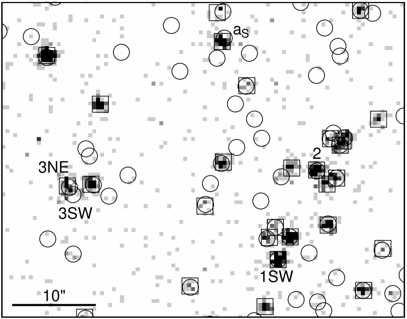
Figure 3: Expanded view of the cloud core region ($50^{\prime\prime}\times 50^{\prime\prime}$). Circles and squares are plot of the infrared and X-ray source positions, respectively. The four X-ray bright high mass YSOs (see text) are indicated by ${\rm a_{S}}$, 1SW, 2, 3NE and 3SW.

To study the X-ray properties of four high mass stars (IRS 1SW, IRS 2, IRS 3NE and ${\rm a_{S}}$) in further detail, we show a closed-up version of the X-ray images of an area $50^{\prime\prime}\times 50^{\prime\prime}$ (Figure 3). The X-ray spectrum of IRS 1SW (No. 79 in Table 1) is fitted with a thin thermal plasma model as is shown in Figure 4a. The best-fit plasma temperature, absorption column density and X-ray luminosity are $\sim$ 2 keV, $\sim 5\times 10^{22}$ cm^-2, and $10^{31}$ ergs s^-1, respectively. The X-rays are time variable with a flare-like event as is shown in Figure 5a.

The X-ray spectrum and light curve of another candidate of the high mass ZAMS star ${\rm a_{S}}$ (No. 91) are given in Figure 4b and 5b, respectively. The X-ray spectrum is well fitted with a thin thermal plasma model (see Figure 4b) with the best-fit plasma temperature, absorption column and X-ray luminosity of $\sim$ 2 keV, $\sim 5\times 10^{22}$ cm^-2, and $6\times 10^{30}$ ergs s^-1, respectively. A flare-like event is also observed (see Figure 5b). These X-ray features are very similar to those of IRS 1SW.

The X-ray spectrum and light curve of IRS 2 (No. 67) are shown in Figure 4c and 5c, respectively. The spectrum is fitted with a thin thermal plasma of 10.9 keV temperature and absorption column of $\sim 10^{23}~{}{\rm cm}^{-2}$ (see Figure 4c). The X-ray flux is highly variable with a slow-rise profile at the peak luminosity of $2\times 10^{31}{\rm ergs~{}s^{-1}}$ (see Figure 5c).

In contrast to the other high mass YSO candidates, the spectrum of IRS 3NE (No. 116) shows no large absorption with the best-fit $N_{\rm H}$ of $1.4\times 10^{22}~{}{\rm cm^{-2}}$, which is inconsistent with the $H-K$ values (see the next section). One possibility is that the spectrum is contaminated by other unknown sources. In Figure 3, we find a faint diffuse or multiple sources near IRS 3NE. We thus re-fit the spectrum with a strongly absorbed high temperature component plus a less absorbed low temperature component; the former is likely from IRS 3NE, and the latter would be another source around. For the spectral fitting, we assume the $N_{\rm H}$ of IRS 3NE to be $7\times 10^{22}~{}{\rm cm^{-2}}$ using the relation of Figure 6 (see the next section). The best-fit two-temperature model is given in Figure 4d. The high temperature component (that from IRS 3NE) has $kT$ $>$ 3.3 keV and the luminosity is estimated to be $1.6\times 10^{30}~{}{\rm ergs~{}s^{-1}}$. Note that the values in Table 1 are the results of one-component fit, hence are different from those of the two-component fit. Since the soft X-ray band of IRS 3NE is largely contaminated by nearby sources, we make the X-ray light curve in the hard (2–10 keV) band and is given in Figure 5d. Unlike the other high mass YSOs, the light curve shows no significant time variability. However, the poor statistics can not give strong constraint on the time variability.

4 DISCUSSION

4.1 Global Features

In Figure 6, we plot the best-fit $N_{\rm H}$ as a function of $H-K$ magnitude, where the bright sources (temperatures are free parameters) are given by circles and those of faint (fixed temperature of 3 keV) are shown by boxes. The best-fit relation for the brighter sources with more than 60 counts (filled circles) is $N_{\rm H}=[(2.04\pm 0.26)(H-K)-(0.64\pm 0.26)]\times 10^{22}~{}{\rm cm^{-2}}$.

Although the intrinsic $H-K$ value for the stars change with their ages and masses, we assume their intrinsic colors are the same. Then, from the relation between $A_{V}$ and infrared extinction (Cohen et al. 1981), we obtain a relation of $N_{\rm H}=(1.32\pm 0.17)\times 10^{21}A_{V}~{}{\rm cm^{-2}}$, significantly different from that in our Galaxy, $N_{\rm H}=1.79\times 10^{21}A_{V}~{}{\rm cm^{-2}}$ (Predehl & Schmitt 1995). This means that the dust-to-gas ratio in this cloud is larger than the mean interstellar medium. We also derived the average intrinsic color to be $H_{0}-K_{0}\sim 0.3$.

We estimate extinction corrected $K$-magnitude ($K$c) using the standard relation of $A_{K}=1.38E(H-K)$ (Cohen et al. 1981). Figure 7 is a scatter plot of $L_{\rm X}$ vs. $K$c, where the symbols are the same as in Figure 6. Although the conversion of $K$c to the stellar mass is not unique, the smaller $K$c represents, as the first approximation, the higher mass stars. From Figure 7, we find that $L_{\rm X}$ seems to saturate at $\sim 10^{31}$ ergs s^-1 in the high mass end.

4.2 High Mass YSOs

We discover heavily absorbed X-rays from high mass YSOs (ZAMS and PMS), IRS 1SW, IRS 2, IRS 3NE and ${\rm a_{S}}$, but no X-rays from IRS 3SW and IRS 5. Garmire et al. (2000) reported the detection of X-rays from “Source n” in the Orion Nebula. The IR luminosity is comparable to our predicted value of high mass stars in Mon R2. Since “Source n” is known to have an H II region (Gezari, Backman, & Werner 1998), it would be already a MS star, possibly ZAMS. The other X-ray emitting high mass stars (Schulz et al. 2001), the Orion Trapezium, are also well in the MS phase. Therefore our observation of Mon R2 provides the first reliable detection of X-rays from high mass YSOs in the cloud cores.

IRS 1SW and ${\rm a_{S}}$ are strong and heavily absorbed X-ray sources, consistent with their $H-K$ values (see Figure 2). The high temperature plasma of $\sim$ 2 keV, large absorption and rapid time variability, in particular flares, are typical of the embedded low mass stars, which show magnetic activity (e.g. Imanishi et al. 2001). In fact, X-rays from high mass MS stars, originated in the stellar wind activity, exhibit lower temperature plasma of $\sim$1 keV and relatively stable light curve (Berghöfer et al. 1997). The X-ray luminosities are comparable to the empirical relation of $L_{\rm X}\sim 10^{-6}$–$10^{-7}\times L_{\rm bol}$ found for stellar wind origin of high mass MS stars (Berghöfer et al. 1997), but are significantly larger than those of low mass YSOs (Feigelson et al. 1993; Casanova et al. 1995). We thus suspect IRS 1SW and ${\rm a_{S}}$ possibly in ZAMS (Aspin & Walther 1990), still dominate the magnetic activity over that of the stellar wind found in high mass MS stars.

IRS 2 exhibits the highest plasma temperature and the largest absorption column density among the bright sources in the Mon R2 cloud. These large values have been only found in the class I low mass stars (Koyama et al. 1996; Imanishi et al. 2001). The relation between the X-ray luminosity and the bolometric luminosity of IRS 2 is also comparable to the empirical relation for stellar wind origin of high mass MS stars (Berghöfer et al. 1997). Although possible source confusion can not be excluded, ASCA found a big flare from the position of IRS 2, with the peak luminosity of $10^{33}~{}{\rm ergs~{}s^{-1}}$ (Hamaguchi et al. 2000). Since the time scale of X-ray variations from IRS 2 (Figure 5c) is long enough to be caused by rotational modulation, it may be conceivable that X-rays arise from the interaction of stellar wind with magnetosphere (e.g. Gagné et al. 1997). However, IRS 2 has no H II region, hence no strong UV field, nor strong stellar wind. Therefore, the more likely scenario is that X-rays from IRS 2 are due to a solar-like magnetic reconnection.

We find heavily-absorbed hard X-rays from IRS 3NE in the outflow source IRS 3 complex (NE and SW). The X-ray luminosity has a relation of $L_{\rm X}\sim 10^{-8}\times L_{\rm bol}$, significantly smaller than the other stars. Since there are no reliable K-band photometry data of IRS 3NE and SW at present, we estimate their K-band magnitude from the 2MASS data, assuming they have the same K-band magnitude. Then IR extinction is very large in the range of $H-K=3-4$ mag. The outflows found from IRS 3 would be derived by magnetic fields, and the infrared polarimetry revealed that the interstellar magnetic field is compressed from the neighbor of the GMCs (e.g. Yao et al. 1997), therefore the X-rays due to the magnetic reconnection between the accretion disk and the star surface are conceivable (Hayashi, Shibata, & Matsumoto 1996). To confirm this scenario, a flare detection is essential. Although we find a hint of rapid flares in Figure 5d, these are not statistically significant.

We have suggested that the high mass PMS have magnetically driven activity similar to that seen in low mass PMS stars. Much of this interpretation arises from the high plasma temperatures and flare-like behavior of the X-ray time series (Figure 5). Since the majority of stars in the universe seem to form binary pairs, one may argue that these high mass YSOs are binaries with low mass companions, and the low mass YSOs may be the origin of the X-ray flares and, in some cases, the entire X-ray flux. The X-ray luminosity of these high mass YSOs, $\sim 10^{30-31}$ ergs s^-1, are however significantly larger than those of typical low mass YSOs of $\sim 10^{28-29}$ ergs s^-1. Thus contribution of low mass companion, if any, may be small fraction of the bulk X-rays observed from the high mass YSOs.

The high mass YSOs in Mon R2 can be compared to the Orion Trapezium stars, $\theta^{1}$ Ori A–E. Since the Trapezium stars are producing luminous H II regions, they already entered the MS phase with very strong stellar winds. Schulz et al. (2001) reported that three of the trapezium stars, C (O7V), E (B0.5) and A (B0V-B1V) exhibit X-rays with the luminosities of about $2\times 10^{32}$ ergs s^-1, $4\times 10^{31}$ ergs s^-1, and $2\times 10^{31}$ ergs s^-1, respectively. They also show a high temperature component of about 2 keV in addition to a lower temperature component of about 1 keV. The luminosities and temperatures of the soft components are consistent with the stellar wind origin. For the hard components, however, the plasma temperature is higher than that predicted with the stellar wind velocity, hence would be attributable to a magnetic origin, like the Mon R2 stars. Moreover, Gagné et al. (1997) found X-ray variations from $\theta^{1}$ Ori C. This would be supporting evidence for remaining the magnetic activity on these high mass stars, although Gagné et al. (1997) interpreted it as the interaction of a magnetosphere and the stellar winds.

Thus we propose a working hypothesis for the study of X-ray evolution of young stars which was proposed in the X-ray study of intermediate mass young stars Herbig Ae/Be stars (Hamaguchi 2001), that, even high mass stars, produce variable and hard (2–3 keV) X-rays due to the magnetic activity between the accretion disk and the stellar surface in a PMS phase (IRS 2 and IRS 3NE). It continues until a ZAMS phase (IRS 1SW and ${\rm a_{S}}$), then gradually stellar wind activities come in (the Trapezium stars). The magnetic activity fades as the accretion disk disappears. Finally most of high mass MS stars emit soft (1 keV) X-rays by the strong stellar wind.

Figure 1: ACIS-I image of the Mon R2 cloud. Red and blue colors represent photons in the soft (0.5–2.0 keV) and hard (2.0–10.0 keV) X-ray bands, respectively. CS $J=5\rightarrow 4$ line intensity map (Choi et al. 2000) is overlaid (white contours).

Figure 2: Plot of the K-mag and $H-K$ mag relation. For the H-band non-detection sources, we assume their $H$-band magnitude to be 17.6, the completeness limit (Carpenter et al. 1997). Open circles are the X-ray detected, and filled circles are non-detected sources. The radius of the open circles gives logarithmic of the X-ray flux. The solid and dashed lines represent time history of stars of 2.5 M_⊙ and reddening vectors at the ages of 0.07 and 2 Myr, respectively.

Figure 4: X-ray spectra and the best-fit thin thermal model for high mass stars. The best-fit two component model is shown for IRS 3NE. (a): IRS 1SW; (b): ${\rm a_{S}}$; (c): IRS 2; (d): IRS 3NE

Figure 5: Light curves of the high mass YSOs in the 0.5–10 keV band. For IRS 3NE (d), the energy band is 2–10 keV. The horizontal axis is the time from the observation start (MJD = 51880.97) and the vertical axis is the ACIS-I counts per ks. (a):IRS 1SW; (b):${\rm a_{S}}$; (c):IRS 2; (d):IRS 3NE

Figure 6: Plots of the absorption column ($N_{\rm H}$) and the near-infrared color ($H-K$) relation. Stars, circles and boxes represent the bright sources (more than 20 counts, temperature is free parameters) and faint sources (less than 20 counts, temperature is fixed to 3 keV, see text), respectively. The solid line is the best-fit relation using the bright sources (filled circles) with more than 60 counts. Typical 1 $\sigma$ errors of $N_{\rm H}$ are separately shown for the filled circles (more than 60 counts) and open circle (20–60 counts) sources.

Figure 7: Plots of the extinction corrected $K$-mag ($K$c) and $L_{\rm X}$ relation. Symbols are the same as in Figure 6. The filled star represent the result of IRS 3NE with a 2-components model (see text). Typical 1 $\sigma$ errors of $L_{\rm X}$ in logarithmic scale is also shown.

Table 1: Chandra X-ray sources in the Monoceros R2 region

No.	R.A.a	Dec.a	Cts	V.P.b	$kT$	$\log({\rm EM})$	$N_{\rm H}$	Fluxc	$\log(L_{\rm X})^{\rm d}$	IRe	Namesf
	(2000)	(2000)		(%)	(keV)	(${\rm cm^{-3}}$)	($\times 10^{22}~{}{\rm cm^{-2}}$)		(${\rm ergs~{}s^{-1}}$)
1	06 07 40.53	-06 22 45.7	16	44.0	3.0(fixed)	53.5(53.1–53.9)	1.6(0.6–3.4)	2.0	29.5(29.2–29.7)	1
2	06 07 40.57	-06 23 56.7	26	99.2	3.1($>$0.9)	53.7(53.2–54.7)	2.0(0.7–4.6)	3.5	29.8(29.6–30.5)
3	06 07 40.63	-06 22 59.2	14	100.0	3.0(fixed)	53.7(53.2–54.2)	3.9(1.7–7.9)	2.2	29.7(29.3–29.8)
4	06 07 40.85	-06 24 04.8	22	84.4	1.6(0.7–9.9)	54.0(53.3–54.8)	2.2(0.9–4.5)	2.3	29.9(29.5–30.7)	6
5	06 07 40.87	-06 21 17.2	22	60.2	12.8($>$1.2)	53.3(53.1–54.2)	0.8(0.2–3.0)	3.7	29.6(29.4–30.0)	3
6	06 07 40.96	-06 24 09.9	11	83.3	3.0(fixed)	53.2(52.7–53.6)	1.0(0.1–3.6)	1.3	29.3(28.8–29.6)	9
7	06 07 41.07	-06 24 08.8	30	89.7	2.6($>$0.5)	54.1(53.2–56.5)	4.3(0.5–73.2)	4.4	30.1(29.6–37.0)	13
8	06 07 41.38	-06 22 12.4	99	99.5	1.6(1.2–2.5)	54.9(54.5–55.2)	3.7(2.6–4.8)	14.2	30.8(30.6–31.1)	19
9	06 07 42.10	-06 23 24.5	9	30.4	3.0(fixed)	53.6(53.0–54.3)	5.3(1.4–16.6)	1.8	29.7(29.1–30.0)
10	06 07 42.13	-06 22 55.3	24	84.7	4.8($>$1.1)	53.6(53.2–54.5)	1.8(0.8–4.5)	3.9	29.8(29.6–30.3)	25
11	06 07 42.20	-06 23 10.9	10	57.1	3.0(fixed)	53.6(53.0–54.2)	4.1(1.3–22.4)	1.9	29.7(29.1–30.2)	27
12	06 07 42.22	-06 23 20.3	10	63.3	3.0(fixed)	54.7(54.0–55.3)	47.6(17.1–105.9)	5.2	30.8(30.1–31.3)
13	06 07 42.27	-06 22 53.6	25	78.0	4.2($>$1.4)	53.8(53.4–54.5)	3.6(1.3–7.9)	4.6	30.0(29.7–30.3)	29
14	06 07 42.40	-06 23 49.8	19	58.7	3.0(fixed)	53.2(52.5–53.5)	1.4(0.1–3.0)	1.2	29.3(28.6–29.4)	32
15	06 07 42.43	-06 23 14.6	7	93.7	3.0(fixed)	53.5(52.0–53.9)	5.0(0.0–20.5)	1.2	29.5(28.3–29.8)	34
16	06 07 42.73	-06 23 07.7	14	99.5	3.0(fixed)	53.2(52.8–53.6)	1.0(0.2–3.3)	1.3	29.3(28.9–29.6)	39
17	06 07 42.84	-06 23 11.5	17	89.3	3.0(fixed)	53.6(53.2–53.9)	2.8(1.2–6.9)	2.3	29.7(29.3–29.9)	43
18	06 07 42.96	-06 22 48.3	9	100.0	3.0(fixed)	54.3(53.3–55.6)	25.6(4.7–160.5)	3.1	30.3(29.4–31.7)	47
19	06 07 42.97	-06 23 21.1	13	32.6	3.0(fixed)	53.4(52.9–53.8)	2.2(0.6–8.6)	1.6	29.5(29.0–29.8)	48
20	06 07 42.99	-06 22 33.8	13	36.3	3.0(fixed)	53.2(52.5–53.8)	0.9(0.0–7.4)	1.2	29.2(28.7–29.8)	50
21	06 07 43.00	-06 24 10.4	27	100.0	3.8($>$0.7)	54.1(53.5–56.8)	6.2(1.9–39.6)	6.1	30.2(29.8–32.7)	54
22	06 07 43.10	-06 22 06.4	19	96.7	3.0(fixed)	53.7(53.1–53.9)	2.2(0.6–4.4)	2.7	29.7(29.2–29.9)	56
23	06 07 43.11	-06 23 56.9	13	93.9	3.0(fixed)	53.2(52.7–53.5)	0.9(0.1–3.4)	1.2	29.3(28.8–29.6)	58
24	06 07 43.23	-06 22 58.0	13	50.5	3.0(fixed)	53.9(53.5–54.2)	7.0(3.2–15.2)	2.9	30.0(29.6–30.2)
25	06 07 43.54	-06 22 44.7	16	38.9	3.0(fixed)	53.2(52.8–53.5)	1.0(0.3–2.2)	1.3	29.3(28.9–29.4)	66
26	06 07 43.58	-06 22 51.7	70	99.5	3.1(1.6–6.5)	54.1(53.8–54.4)	1.1(0.7–1.8)	8.7	30.1(30.0–30.3)	70	${\rm d_{N}}$
27	06 07 43.58	-06 23 21.8	30	98.2	0.0($>$2.2)g	53.9(53.7–54.2)	5.6(3.0–12.5)	10.0	30.2(30.0–30.3)	65
28	06 07 43.61	-06 23 10.6	14	84.5	3.0(fixed)	53.5(53.1–53.8)	1.9(0.9–4.1)	2.1	29.6(29.3–29.8)	75
29	06 07 43.66	-06 24 21.7	10	87.1	3.0(fixed)	53.2(52.5–53.6)	1.0(0.1–4.4)	1.1	29.2(28.6–29.6)	78
30	06 07 43.69	-06 23 01.6	30	61.8	6.9($>$1.3)	54.3(53.9–55.9)	20.4(7.7–53.9)	11.0	30.6(30.1–31.5)
31	06 07 43.72	-06 22 46.8	26	53.3	1.4(0.8–2.6)	54.1(53.5–54.8)	2.3(1.0–4.5)	2.6	30.0(29.6–30.6)	79
32	06 07 43.86	-06 23 27.1	9	99.2	3.0(fixed)	53.2(52.5–53.9)	1.6(0.1–12.9)	1.2	29.3(28.6–29.9)	86
33	06 07 43.92	-06 23 13.3	36	94.8	3.6($>$1.2)	54.2(53.7–55.2)	5.5(2.2–12.3)	7.7	30.3(30.0–31.0)	87
34	06 07 43.96	-06 23 27.1	10	56.0	3.0(fixed)	53.7(53.0–54.3)	5.4(1.5–28.1)	2.0	29.7(29.1–30.3)
35	06 07 44.14	-06 24 20.5	44	63.0	1.3(0.8–2.2)	54.7(54.1–55.3)	4.1(2.8–6.4)	5.6	30.6(30.2–31.2)	93
36	06 07 44.21	-06 23 32.0	14	99.4	3.0(fixed)	54.1(53.7–54.4)	11.9(5.5–23.8)	3.6	30.2(29.8–30.4)
37	06 07 44.21	-06 23 25.4	14	65.6	3.0(fixed)	53.4(52.9–53.7)	1.2(0.3–3.4)	1.7	29.4(29.0–29.7)	95
38	06 07 44.23	-06 22 30.7	33	95.7	22.9($>$1.0)	53.3(53.0–53.5)	0.2(0.0–2.0)	3.8	29.5(29.5–30.1)	94
39	06 07 44.29	-06 24 22.5	7	89.1	3.0(fixed)	52.8(52.0–53.1)	0.5(0.0–2.3)	0.6	28.9(28.5–29.0)	97
40	06 07 44.46	-06 22 41.3	42	96.6	2.7(1.2–17.8)	54.0(53.6–54.7)	2.2(0.9–4.3)	5.7	30.1(29.9–30.6)	103
41	06 07 44.49	-06 22 33.8	273	100.0	4.3(2.8–16.7)	55.1(54.8–55.3)	5.9(4.4–7.1)	72.7	31.2(31.1–31.3)
42	06 07 44.52	-06 23 21.7	24	66.1	2.1($>$0.4)	53.6(53.0–55.7)	1.3(0.2–4.9)	2.0	29.6(29.4–31.5)	105
43	06 07 44.53	-06 22 53.0	12	92.3	3.0(fixed)	53.9(53.4–54.3)	7.2(2.9–22.6)	2.8	30.0(29.5–30.3)
44	06 07 44.60	-06 23 15.5	14	58.6	3.0(fixed)	53.7(53.2–54.0)	4.2(1.9–9.6)	2.3	29.8(29.4–29.9)	107
45	06 07 44.73	-06 23 42.3	92	99.1	1.9(1.1–2.8)	54.6(54.2–55.0)	2.3(1.7–3.6)	11.5	30.5(30.4–30.9)
46	06 07 44.79	-06 24 05.2	12	66.8	3.0(fixed)	53.3(52.7–53.6)	1.6(0.4–4.2)	1.3	29.3(28.8–29.5)	118
47	06 07 44.79	-06 23 26.1	5	84.7	3.0(fixed)	53.4(51.9–54.0)	4.4(0.0–35.7)	1.1	29.4(28.3–30.0)	122
48	06 07 44.81	-06 23 35.9	16	63.5	3.0(fixed)	53.9(53.5–54.2)	6.5(3.4–13.4)	3.3	30.0(29.7–30.2)	116
49	06 07 44.94	-06 22 40.0	21	83.6	3.2(0.9–19.2)	53.4(53.0–54.1)	0.8(0.1–2.5)	2.2	29.5(29.3–29.9)	119
50	06 07 44.95	-06 23 26.0	5	62.3	3.0(fixed)	53.1(51.9–53.6)	2.3(0.0–17.5)	0.8	29.2(28.3–29.6)	153
51	06 07 45.22	-06 23 28.3	54	80.3	2.7(1.3–9.0)	54.2(53.8–54.7)	2.5(1.5–4.0)	8.5	30.3(30.1–30.6)	131
52	06 07 45.23	-06 23 03.3	12	49.0	3.0(fixed)	53.7(53.1–54.6)	4.2(1.4–45.0)	2.1	29.7(29.2–30.7)	132
53	06 07 45.25	-06 23 19.9	10	99.2	3.0(fixed)	53.0(52.5–53.3)	0.6(0.0–1.8)	1.0	29.1(28.6–29.3)	139	IRS 4
54	06 07 45.25	-06 23 35.5	24	97.9	3.3($>$0.5)	53.9(53.3–56.4)	3.7(1.2–13.9)	3.9	29.9(29.6–32.1)	134
55	06 07 45.27	-06 22 47.2	30	87.4	2.0(0.8–5.2)	54.3(53.6–55.5)	4.5(2.4–10.2)	5.1	30.3(29.9–31.4)
56	06 07 45.30	-06 22 28.3	24	84.4	2.4(0.9–13.8)	53.3(52.9–54.0)	0.3(0.0–1.5)	1.8	29.3(29.2–29.9)
57	06 07 45.39	-06 23 08.5	42	100.0	59.2($>$3.0)	54.0(53.8–54.2)	3.7(2.4–7.6)	12.7	30.2(30.1–30.4)	142
58	06 07 45.42	-06 22 33.7	33	83.9	2.4(1.0–8.4)	54.3(53.7–55.2)	4.3(2.3–8.8)	6.2	30.3(30.0–31.0)	143
59	06 07 45.46	-06 21 28.4	67	58.5	1.8(0.9–3.0)	54.3(53.9–55.0)	1.8(0.9–3.5)	6.9	30.2(30.0–30.9)	146
60	06 07 45.47	-06 23 16.5	24	84.6	1.6(0.7–4.1)	53.8(53.2–54.5)	1.4(0.6–3.2)	2.0	29.7(29.4–30.3)	147
61	06 07 45.57	-06 22 49.9	86	98.5	2.0(1.5–3.8)	54.8(54.4–55.3)	4.7(3.2–6.8)	15.5	30.8(30.5–31.2)	150
62	06 07 45.59	-06 22 50.5	74	99.4	1.6(0.9–3.5)	54.8(54.2–55.5)	4.9(3.2–7.2)	11.2	30.8(30.4–31.4)	160
63	06 07 45.62	-06 22 54.6	40	100.0	0.0($>$4.4)g	54.0(53.8–54.2)	5.6(3.2–13.4)	12.3	30.3(30.1–30.4)	167
64	06 07 45.67	-06 22 49.7	49	78.7	2.5(1.4–6.9)	54.4(53.9–55.0)	4.0(2.4–6.6)	8.7	30.4(30.1–30.9)	197	${\rm c_{S}}$
65	06 07 45.69	-06 23 00.4	67	99.2	2.0(1.1–3.9)	54.9(54.4–55.6)	8.0(5.1–12.7)	14.5	30.9(30.5–31.5)	169
66	06 07 45.70	-06 22 55.3	50	99.8	7.8($>$2.0)	54.2(53.9–54.8)	5.3(2.9–9.9)	14.2	30.4(30.2–30.7)
67	06 07 45.79	-06 22 53.6	99	99.3	10.9($>$2.0)	54.6(54.4–55.3)	9.1(5.7–16.9)	35.4	30.8(30.7–31.3)	178	IRS 2
68	06 07 45.83	-06 21 46.6	541	98.5	2.0(1.7–2.3)	55.1(55.0–55.3)	1.4(1.2–1.6)	60.8	31.1(31.0–31.2)	181
69	06 07 45.88	-06 21 54.3	34	56.3	0.5(0.1–0.8)	53.1(52.9–58.9)	0.0(0.0–0.9)	1.2	29.0(29.0–31.6)	184
70	06 07 45.90	-06 24 00.9	84	99.7	6.0($>$1.5)	54.8(54.5–55.5)	15.0(8.9–27.4)	33.3	31.0(30.8–31.7)
71	06 07 45.94	-06 23 32.6	83	74.1	2.7(1.6–5.4)	54.5(54.1–54.8)	2.8(1.8–4.0)	13.9	30.5(30.3–30.8)	192
72	06 07 45.99	-06 22 53.3	34	56.0	2.5($>$0.6)	54.3(53.7–56.1)	6.2(2.5–13.2)	6.7	30.4(30.0–31.8)
73	06 07 46.00	-06 22 25.7	19	77.6	3.0(fixed)	53.4(53.0–53.6)	0.9(0.4–1.7)	1.8	29.4(29.2–29.5)	210
74	06 07 46.00	-06 23 43.7	14	76.8	3.0(fixed)	53.2(52.8–53.5)	0.8(0.2–2.5)	1.4	29.3(28.9–29.5)	200
75	06 07 46.01	-06 23 01.9	122	100.0	2.8(1.6–4.5)	55.0(54.7–55.5)	7.3(5.5–10.9)	30.5	31.0(30.8–31.4)	199
76	06 07 46.01	-06 22 24.0	40	96.6	1.5(0.8–2.8)	54.2(53.7–54.9)	2.0(0.9–3.7)	3.9	30.1(29.8–30.8)	195	${\rm c_{N}}$
77	06 07 46.04	-06 23 50.2	13	31.9	3.0(fixed)	53.6(53.2–53.9)	3.2(1.4–8.1)	2.2	29.7(29.3–29.9)	203
78	06 07 46.10	-06 22 05.5	116	100.0	7.7($>$3.1)	54.3(54.2–54.6)	2.3(1.3–3.5)	25.5	30.6(30.5–30.7)	204
79	06 07 46.11	-06 23 04.7	130	98.8	1.9(1.3–2.8)	55.0(54.7–55.4)	4.7(3.5–6.4)	22.2	31.0(30.8–31.3)	207	IRS 1SW
80	06 07 46.13	-06 23 00.7	26	53.2	2.0($>$0.6)	54.1(53.4–54.8)	3.9(0.3–8.8)	3.3	30.1(29.4–31.5)	237
81	06 07 46.16	-06 21 30.7	16	85.0	3.0(fixed)	53.2(52.8–53.4)	0.6(0.2–1.4)	1.5	29.3(29.0–29.4)	211
82	06 07 46.18	-06 23 01.9	28	96.5	4.0($>$1.5)	53.1(52.9–53.3)	0.0(0.0–0.2)	2.1	29.2(29.2–29.3)	214	IRS 1NE
83	06 07 46.22	-06 23 10.6	53	80.5	3.8($>$1.2)	54.4(53.9–55.6)	5.8(2.3–18.9)	12.0	30.5(30.2–31.5)
84	06 07 46.34	-06 23 35.4	12	61.8	3.0(fixed)	53.3(52.7–53.5)	1.5(0.3–3.6)	1.2	29.3(28.8–29.5)	223
85	06 07 46.37	-06 22 43.1	15	93.5	3.0(fixed)	53.2(52.8–53.5)	0.9(0.3–2.0)	1.3	29.3(28.9–29.4)	229
86	06 07 46.39	-06 22 24.5	22	41.8	0.0($>$2.4)g	53.2(52.9–53.4)	0.3(0.0–1.0)	3.2	29.5(29.2–29.6)	228
87	06 07 46.52	-06 23 30.2	15	99.7	3.0(fixed)	53.7(53.3–53.9)	2.6(1.3–5.3)	2.6	29.7(29.4–29.9)	290
88	06 07 46.53	-06 23 18.5	14	93.9	3.0(fixed)	54.2(53.4–55.2)	16.4(4.1–90.8)	3.3	30.2(29.6–31.2)
89	06 07 46.54	-06 23 26.7	20	64.7	3.0(fixed)	53.6(53.3–53.8)	2.4(1.3–4.0)	2.5	29.7(29.4–29.8)	235
90	06 07 46.56	-06 22 52.6	45	98.5	3.0(1.4–21.2)	54.1(53.6–54.6)	2.6(1.1–4.3)	6.8	30.1(29.9–30.5)	241
91	06 07 46.57	-06 22 37.6	89	100.0	2.6(1.6–6.2)	54.8(54.3–55.4)	6.0(4.0–9.2)	19.7	30.8(30.6–31.2)	239	${\rm a_{S}}$
92	06 07 46.57	-06 22 19.0	17	99.4	3.0(fixed)	53.8(53.5–54.0)	3.3(2.0–5.8)	3.2	29.9(29.6–30.0)	238
93	06 07 46.62	-06 22 34.0	13	100.0	3.0(fixed)	53.5(53.0–53.8)	2.3(0.9–6.1)	1.8	29.6(29.1–29.8)	240	${\rm a_{N}}$
94	06 07 46.63	-06 23 30.0	27	90.0	2.1(0.7–6.6)	54.2(53.5–55.7)	4.3(2.2–11.6)	4.6	30.2(29.9–31.5)	245
95	06 07 46.68	-06 23 12.9	74	92.5	1.9(1.2–3.1)	54.4(54.1–54.8)	2.0(1.4–3.0)	8.9	30.4(30.2–30.7)	248	${\rm b_{N}}$
96	06 07 46.72	-06 22 58.0	11	87.7	3.0(fixed)	53.5(53.0–53.7)	2.3(0.8–5.0)	1.7	29.5(29.1–29.7)	249
97	06 07 46.84	-06 23 08.0	14	80.1	3.0(fixed)	53.2(52.7–53.4)	0.7(0.1–1.8)	1.3	29.2(28.8–29.4)	250
98	06 07 46.91	-06 24 17.3	31	89.6	3.8(1.6–43.4)	54.0(53.7–54.5)	1.2(0.6–2.6)	9.3	30.1(30.0–30.4)	254
99	06 07 47.04	-06 21 26.6	8	74.1	3.0(fixed)	53.1(52.3–53.4)	0.7(0.0–2.5)	1.0	29.1(28.7–29.3)	260
100	06 07 47.06	-06 23 33.8	32	100.0	2.0(0.4–55.9)	54.4(53.6–57.3)	6.1(2.3–17.2)	5.3	30.4(29.9–33.0)	262	IRS 7
101	06 07 47.12	-06 21 28.3	6	67.4	3.0(fixed)	53.0(52.2–53.4)	0.4(0.0–3.8)	0.9	29.0(28.7–29.4)	263
102	06 07 47.20	-06 22 31.2	57	84.7	5.4(2.3–65.2)	54.2(53.9–54.6)	3.5(2.0–5.8)	13.4	30.4(30.2–30.6)	264	g
103	06 07 47.30	-06 23 47.2	33	86.5	1.1(0.4–2.1)	54.1(53.6–55.3)	1.6(0.8–3.0)	2.3	30.0(29.6–31.2)	267
104	06 07 47.35	-06 21 51.8	119	64.3	2.7(1.6–5.7)	54.8(54.4–55.2)	4.1(2.9–5.7)	23.9	30.8(30.6–31.1)	268
105	06 07 47.48	-06 22 18.7	26	85.8	7.2($>$1.0)	53.7(53.4–55.3)	3.1(1.2–12.7)	5.7	29.9(29.7–31.0)	273
106	06 07 47.49	-06 23 36.4	46	99.7	1.4(0.8–2.3)	54.6(54.0–55.3)	3.5(2.1–5.4)	5.7	30.5(30.1–31.1)	274
107	06 07 47.59	-06 22 45.4	88	100.0	7.1(2.9)	54.5(54.2–55.3)	6.5(4.0–10.8)	24.2	30.7(30.5–31.1)
108	06 07 47.64	-06 24 19.8	56	99.9	3.4(1.8–7.4)	53.9(53.6–54.2)	0.8(0.5–1.5)	6.9	30.0(29.9–30.1)	279
109	06 07 47.66	-06 23 58.6	18	59.5	3.0(fixed)	53.3(53.1–53.6)	0.1(0.0–0.5)	2.9	29.4(29.4–29.6)	277
110	06 07 47.67	-06 22 55.3	70	100.0	4.7(2.8–15.6)	53.8(53.6–54.1)	0.6(0.2–1.2)	8.0	30.0(29.9–30.1)	278
111	06 07 47.72	-06 23 11.9	14	69.7	3.0(fixed)	53.5(53.0–53.7)	1.8(0.7–4.3)	1.9	29.5(29.2–29.7)	283
112	06 07 47.77	-06 21 36.9	14	46.6	3.0(fixed)	53.6(53.1–53.8)	1.2(0.4–2.6)	2.6	29.6(29.2–29.7)	284
113	06 07 47.80	-06 24 09.6	6	86.3	3.0(fixed)	52.9(52.1–53.4)	0.4(0.0–4.5)	0.9	29.0(28.7–29.4)	286
114	06 07 47.81	-06 23 30.9	5	34.0	3.0(fixed)	53.2(51.9–53.8)	3.0(0.0–23.9)	0.9	29.3(28.3–29.8)	210
115	06 07 47.84	-06 21 45.1	15	78.7	3.0(fixed)	53.6(53.2–53.8)	1.4(0.6–2.7)	2.5	29.6(29.3–29.7)	287
116	06 07 47.87	-06 22 55.5	46	68.4	0.0($>$6.2)g	53.8(53.6–53.9)	1.6(0.9–3.1)	9.2	30.0(29.9–30.2)	291	IRS 3NE
117	06 07 47.88	-06 21 41.9	15	100.0	3.0(fixed)	54.1(53.7–54.4)	6.5(3.2–13.3)	4.8	30.2(29.8–30.3)	292
118	06 07 48.03	-06 22 30.8	194	98.8	2.5(1.8–3.7)	55.1(54.9–55.4)	5.2(4.1–6.7)	40.6	31.1(31.0–31.3)	296	e
119	06 07 48.04	-06 22 39.3	244	51.3	2.2(1.7–3.0)	54.6(54.4–54.7)	0.9(0.7–1.1)	22.8	30.6(30.5–30.7)	299	f
120	06 07 48.07	-06 21 22.6	54	48.9	0.0($>$5.6)g	54.6(54.4–54.7)	5.8(3.8–10.4)	44.0	30.8(30.7–31.0)
121	06 07 48.09	-06 23 33.0	19	97.7	3.0(fixed)	54.0(53.6–54.3)	7.9(3.0–17.3)	3.8	30.1(29.7–30.3)
122	06 07 48.35	-06 23 22.4	8	95.0	3.0(fixed)	53.3(52.2–53.6)	2.5(0.0–8.5)	1.1	29.3(28.4–29.5)
123	06 07 48.55	-06 21 32.2	9	92.8	3.0(fixed)	53.2(52.5–53.5)	0.4(0.0–1.9)	1.4	29.2(28.9–29.5)	317
124	06 07 48.64	-06 23 40.5	9	97.6	3.0(fixed)	53.8(53.1–54.1)	4.1(1.0–11.8)	2.7	29.8(29.2–30.0)	320
125	06 07 48.68	-06 24 06.3	128	100.0	3.2(2.1–6.0)	54.6(54.3–54.9)	2.0(1.4–2.9)	25.8	30.7(30.6–30.8)	325
126	06 07 48.69	-06 22 27.4	99	98.2	7.6(3.3–69.9)	54.1(54.0–54.4)	1.5(0.9–2.3)	18.1	30.4(30.3–30.5)	323
127	06 07 48.83	-06 22 21.8	14	55.9	3.0(fixed)	53.2(52.5–53.6)	0.8(0.0–3.1)	1.2	29.2(28.8–29.5)	328
128	06 07 49.03	-06 21 39.7	83	96.9	5.9(2.7–23.9)	54.2(54.0–54.4)	0.6(0.3–1.1)	20.4	30.4(30.3–30.4)	332
129	06 07 49.07	-06 22 17.7	8	75.9	3.0(fixed)	52.4(51.2–52.7)	0.0(0.0–0.0)	0.3	28.4(28.4–28.4)	334
130	06 07 49.07	-06 24 22.7	159	96.4	1.9(1.5–2.5)	54.1(54.0–54.2)	0.2(0.1–0.4)	10.3	30.1(30.0–30.1)	336
131	06 07 49.25	-06 22 48.1	9	74.9	3.0(fixed)	53.3(52.8–53.6)	2.0(0.4–4.9)	1.3	29.4(28.8–29.5)
132	06 07 49.37	-06 23 54.3	8	68.5	3.0(fixed)	53.6(52.7–54.0)	2.8(0.2–13.5)	2.0	29.6(28.8–30.0)
133	06 07 49.62	-06 23 22.8	11	78.3	3.0(fixed)	53.5(53.0–53.8)	2.6(0.9–7.0)	1.8	29.6(29.1–29.8)	345
134	06 07 49.65	-06 21 42.6	60	100.0	3.7(1.6–9.1)	54.0(53.7–54.3)	0.7(0.4–1.4)	9.3	30.1(30.0–30.3)	346
135	06 07 49.82	-06 21 14.0	29	67.2	1.4(0.7–3.1)	53.9(53.4–54.7)	1.4(0.7–2.7)	2.4	29.8(29.6–30.5)	349
136	06 07 49.93	-06 22 10.8	8	70.4	3.0(fixed)	53.2(52.6–53.6)	0.2(0.0–2.3)	1.6	29.2(29.1–29.6)	352
137	06 07 49.97	-06 23 20.1	23	97.5	1.0(0.4–2.2)	54.4(53.7–55.7)	2.8(1.3–5.4)	2.5	30.3(29.7–31.3)	353
138	06 07 50.06	-06 22 36.0	9	84.9	3.0(fixed)	53.5(52.8–53.8)	3.8(0.9–11.1)	1.6	29.6(28.9–29.8)	354
139	06 07 50.35	-06 23 46.9	10	89.2	3.0(fixed)	53.4(52.9–53.7)	2.4(0.0–8.8)	1.4	29.5(28.5–29.7)	355
140	06 07 50.43	-06 24 05.0	11	58.7	3.0(fixed)	53.0(52.5–53.3)	0.5(0.0–1.7)	1.0	29.1(28.7–29.3)	358
141	06 07 50.57	-06 24 01.9	7	67.3	3.0(fixed)	52.8(51.4–53.3)	0.9(0.0–5.6)	0.5	28.8(28.4–29.0)	361
142	06 07 50.58	-06 23 28.5	16	59.3	3.0(fixed)	53.4(53.0–53.7)	0.1(0.0–0.8)	3.1	29.5(29.4–29.7)	360
143	06 07 50.75	-06 23 23.1	6	96.9	3.0(fixed)	52.8(52.2–53.3)	0.0(0.0–0.0)	0.9	28.9(28.9–28.9)	362
144	06 07 51.00	-06 22 60.0	9	74.2	3.0(fixed)	53.5(52.8–54.1)	3.1(0.7–22.7)	1.5	29.5(28.9–30.2)	364
145	06 07 51.04	-06 22 24.3	7	53.1	3.0(fixed)	53.6(52.3–54.0)	2.1(0.0–16.2)	2.2	29.6(28.8–30.0)	366
146	06 07 51.39	-06 21 44.5	26	97.3	1.8(0.6–5.1)	53.4(53.2–54.5)	0.5(0.1–2.2)	1.6	29.4(29.2–30.3)	369
147	06 07 51.70	-06 23 18.1	79	87.1	2.7(1.6–5.8)	55.0(54.7–55.4)	1.7(1.1–2.6)	61.8	31.1(30.9–31.3)	372
148	06 07 51.74	-06 21 29.8	96	99.9	3.1(1.5–6.6)	54.3(53.9–54.7)	1.5(0.9–2.6)	12.7	30.3(30.2–30.6)	374
149	06 07 52.17	-06 21 17.7	68	90.0	2.1(1.2–3.2)	53.6(53.5–53.9)	0.2(0.0–0.4)	4.1	29.6(29.5–29.7)	378
150	06 07 52.25	-06 21 38.5	70	87.4	1.5(1.1–2.1)	53.8(53.6–54.5)	0.3(0.1–1.0)	4.2	29.7(29.6–30.3)	379
151	06 07 52.28	-06 21 18.2	69	35.0	2.1(1.2–3.6)	53.7(53.5–53.9)	0.2(0.1–0.5)	4.3	29.7(29.6–29.8)	380
152	06 07 52.30	-06 23 46.5	12	98.7	3.0(fixed)	53.3(52.9–53.6)	1.4(0.4–3.1)	1.5	29.4(29.0–29.6)	381
153	06 07 52.38	-06 22 57.4	10	62.7	3.0(fixed)	53.4(53.0–53.7)	0.0(0.0–0.8)	3.5	29.5(29.4–29.7)	382
154	06 07 52.91	-06 23 27.6	11	88.8	3.0(fixed)	52.7(52.3–52.9)	0.0(0.0–0.0)	0.7	28.8(28.8–28.8)	386

Note. — Parentheses indicate the 90% confidence limits.

References

- (1) Aspin, C., & Walther, D.M. 1990, A&A, 235, 387
- (2) Berghöfer, T.W., Schmitt, J.H.M.M., Danner, R., & Cassinelli, J.P. 1997, A&A, 322, 167
- (3) Carpenter, J.M., Meyer, M.R., Dougados, C., Strom, S.E., & Hillenbrand L.A. 1997, AJ, 114, 198
- (4) Casanova, S., Montmerle, T., Feigelson, E.D., & André, P. 1995, ApJ, 439, 752
- (5) Choi, M., Evans II, N.J., Tafalla, M., & Bachiller, R. 2000, ApJ, 538, 738
- (6) Cohen, J.G., & Frogel, J.A. 1977, ApJ, 211, 178
- (7) Cohen, J.G., Frogel, J.A., Persson, S.E., & Elias, J.H. 1981, ApJ, 249, 481
- (8) D’Antona, F., & Mazzitelli, I. 1994, ApJS, 90, 467
- (9) Feigelson, E.D., & DeCampli, W.M. 1981, ApJ, 243, L89
- (10) Feigelson, E.D., Casanova, S., Montmerle, T., Guibert, J. 1993, ApJ, 416, 623
- (11) Gagné, M., Caillault, J.P., Stauffer, J.R., & Linsky, J.L. 1997, ApJ, 478, L87
- (12) Garmire, G., Feigelson, E.D., Broos, P., Hillenbrand, L.A., Pravdo, S.H., Townsley, L., & Tsuboi, Y. 2000, AJ, 120, 1426
- (13) Gezari, D.Y., Backman, D.E., & Werner, M.W. 1998, ApJ, 509, 283
- (14) Giannakopoulou, J., Mitchell, G.F., Hasegawa, T.I., Matthews, H.E., & Maillard, J.P. 1997, ApJ, 487, 346
- (15) Hamaguchi, K., Tsuboi, Y., & Koyama, K. 2000, Adv. Space Res., 25, 531
- (16) Hamaguchi, K. 2001, Ph.D. Thesis, Kyoto University
- (17) Hayashi, M.R., Shibata, K., & Matsumoto, R. 1996, ApJ, 468, L37
- (18) Henning, Th., Chini, R., & Pfau, W. 1992, A&A, 263, 285
- (19) Hough, J.H., Chrysostomou, A., Messinger, D.W., Whittet, D.C.B., Aitken, D.K., & Roche, P.F. 1996, ApJ, 461, 902
- (20) Hofner, P., & Churchwell, E. 1997, ApJ, 486, L39
- (21) Howard, E.M., Pipher, J.L., & Forrest, W.J. 1994, ApJ, 425, 707
- (22) Imanishi, K., Koyama, K., & Tsuboi, Y. 2001, ApJ, 557, 747
- (23) Kamata, Y., Koyama, K., Tsuboi, Y., Yamauchi, S. 1997, PASJ, 49, 461
- (24) Koyama, K., Hamaguchi, K., Ueno, S., Kobayashi, N., & Feigelson E.D. 1996, PASJ, 48, L87
- (25) Lucy, L.B., & White R.L. 1980, ApJ, 241, 300
- (26) Massi, M., Felli, M., & Simon, M. 1985, A&A, 152, 387
- (27) Mewe, R., Gronenschild, E.H.B.M., & van den Oord, G.H.J. 1985, A&AS, 62, 197
- (28) Montmerle, T., Koch-Miramond, L., Falgarone, E., & Grindlay, J.E. 1983, ApJ, 269, 182
- (29) Pittard J.M., & Stevens, I.R. 1997, MNRAS, 292, 298
- (30) Predehl, P., & Schmitt, J.H.M.M. 1995, A&A, 293, 889
- (31) Press, W.H., Teukolsky, S.A., Vetterling, W.T., & Flannery, B.P. 1992, Numerical Recipes in C (2d ed; London: Cambridge University Press)
- (32) Racine, R. 1968, AJ, 73, 233
- (33) Schulz, N.S., Canizares, C., Huenemoerder, D., Kastner, J.H., Taylor, S.C., & Bergstrom, E.J. 2001, ApJ, 549, 441
- (34) Sekimoto, Y., Matsuzaki, K., Kamae, T., Tatematsu, K., Yamamoto, S., & Umemoto, T. 2000, PASJ, 52, L31
- (35) Smith, R.G., Sellgren, K., & Tokunaga, A.T. 1989, ApJ, 344, 413
- (36) Smits, D.P., Cohen, R.J., & Hutawarakorn, B. 1998, MNRAS, 296, L11
- (37) Yamauchi, S., Koyama, K., Sakano, M., & Okada, K. 1996, PASJ, 48, 719
- (38) Yao, Y., Hirata, N., Ishii M., Nagata, T., Ogawa, Y., Sato, S., Watanabe, M., & Yamashita, T. 1997, ApJ, 490, 281
- (39) Weisskopf, M.C., Tananbaum, H.D., Van Speybroeck, L.P., & O’Dell, S.L. 2000, Proc. SPIE, 4012, 2