astro-ph/0110460

Quintessence Restrictions on Negative Power
and Condensate Potentials

A. de la Macorra and C. Stephan-Otto

Instituto de Física, UNAM

Apdo. Postal 20-364, 01000 México D.F., México

ABSTRACT

We study the cosmological evolution of scalar fields that arise from a phase transition at some energy scale $\Lambda_{c}$. We focus on negative power potentials given by $V=c\Lambda_{c}^{4+n}\phi^{-n}$ and restrict the cosmological viable values of $\Lambda_{c}$ and $n$. We make a complete analysis of $V$ and impose $SN1a$ conditions on the different cosmological parameters. The cosmological observations ruled out models where the scalar field has reached its attractor solution. For models where this is not the case, the analytic approximated solutions are not good enough to determine whether a specific model is phenomenologically viable or not and the full differential equations must be numerically solved. The results are not fine tuned since a change of $45\%$ on the initial conditions does not spoil the final results. We also determine the values of $N_{c},N_{f}$ that give a condensation scale $\Lambda_{c}$ consistent with gauge coupling unification, leaving only four models that satisfy unification and SN1a constraints.

 

1 INTRODUCTION

Recent cosmological results given by the superonovae project SN1a [1] and the Maxima and Boomerang [2] observations have lead to conclude that the universe is flat and it is expanding with an accelerating velocity. This conclusions show that the universe is now dominated by a energy density with negative pressure with $\Omega_{phi}=0.7\pm.1$ and $w_{\phi}<-2/3$ [3] . This energy is generically called the cosmological constant. An interesting parametrization of this energy density is in terms of a scalar field with gravitationally interaction only called quintessence [4]. The evolution of scalar field has been widely studied and some general approach con be found in [11], [12]. The evolution of the scalar field $\phi$ depends on the functional form of its potential $V$ and a late time accelerating universe constraints the form of the potential [12].

In this paper we will concentrate on negative power potentials because they lead to an acceptable phenomenology and because they are naturally obtained from gauge group dynamics. Negative power potential have been extensively studied [4]-[12] first by [5] and then as tracker fields by [4]. Steinhardt et al. [4] showed that scalar field with a negative power potential $V=c\phi^{-n}$ with $n>5$ has already reached its tracker solution but are not cosmologically acceptable because they have $w_{\phi}>-0.52$. However, if the scalar field has not reached its tracker solution by today, we will show that the models may lead to an acceptable phenomenology and the final results depend on the initial conditions and on the value of $n$. Contrary to the tracker models, no analytic solution is good enough to determine the value of $w_{\phi o}$ (from now on the subscript $o$ will refer to present days values) and it is sensitive to the whole dynamics. We will solve numerically the differential equations and we will constrain the values $n$ of cosmologically viable models, including the big bang nucleosynthesis (NS) constraints [15]. We will also give approximated analytically solutions.

Tracker solutions are widely favored because they do not have a fine tuning problem of initial conditions. But even more, they are independent of the initial conditions since the range of the initial conditions can vary up to 100 orders of magnitude. The models with $n<5$ do depend on the initial conditions but it is important to remark that they do not have a fine tuning problem. The initial conditions can vary up to 45%, the solutions are still fine and the values of the initial conditions are completely ”natural”, i.e. they are of the same order of magnitude as the other relevant cosmological parameters. So, to conclude, one thing is to have a model with no dependence on the initial conditions and another is to have a fine tuning problem. ”Natural” models in physics should not have fine tuning problems but they do in general depend on the initial values as it is the case for our models. However, for any initial conditions we will end up with $-1\leq w_{\phi o}\leq-2/(2+n)=w_{tr}$, where $n$ gives the inverse power and $w_{tr}$ is the tracker value.

Negative power potentials [7]-[10] can be obtained using Affleck et al. (”ADS”) superpotential [16]. The condensation scale $\Lambda_{c}$ of the gauge group $SU(N_{c})$ can be determined from a high energy scale ($\Lambda$) using renormalization group equation in terms of $N_{c},N_{f}$ and it is then naturally to ask if it is possible to have a common gauge coupling unification with the Standard Model (”S.M.”) gauge groups [10]. We will show that this is indeed possible and we will give the values of $N_{c},N_{f}$ where gauge coupling unification is achieved.

The cosmological picture in the case of gauge coupling unification is very pleasing. We would assume gauge coupling unification at a scale $\Lambda$ for all gauge groups (as predicted by string theory) and then let all fields evolve. At the beginning all fields, ”S.M.” and those from the $SU(N_{c})$ gauge group, are massless and redshift as radiation until we reach the condensation scale $\Lambda_{c}$. Below this scale the fields of $SU(N_{c})$ group will dynamically condense and we use ADS potential to study its cosmologically evolution. Interesting enough, the relative energy density of the $SU(N_{c})$ group $\Omega_{\phi}$ drops quickly, independently of the initial conditions, and it is close to zero for a long period of time, which may include nucleosynthesis, until very recently (around one e-fold of inflation). The energy density of the universe is at present time dominated by the scalar field with $\Omega_{\phi}\simeq 0.7$ and a negative pressure $w_{\phi}<-2/3$ leading to an accelerating universe [3].

The paper is organized as follows. In section 2 we give the general frame work to derive the scalar potential for $\phi$ from non-abelian gauge dynamics using ADS potential. In section 3 we analyze the cosmological evolution of $\phi$ and we concentrate in the non attractor regime. We derive analytic formulas for $w_{\phi o}$ and $\phi_{o}$ as a function of the initial conditions and on $n$ and we discuss in detail the possible choices of initial conditions and show that the models do not have a fine tuning problem. In section 4 we constrain the values of $n$ in order to have $w_{\phi o}<-2/3$ while in section 5 we comment on the possibility to have models with a gauge coupling constant unified with the couplings of the standard model and we explicitly give these models. In section 6 we give further examples. Finally, we summarize and conclude in section 7.

2 POTENTIALS OF THE FORM $V=c\Lambda_{c}^{4+n}\phi^{-n}$

In this work we study quintessence field (scalar) $\phi$ with negative power potentials that arise from a phase transition at some stage of the evolution of the universe. The energy scale of the phase transition is given by $\Lambda_{c}$ and the initial value of the scalar field $\phi$ is naturally given by $\phi_{i}=\Lambda_{c}$ since it is the relevant scale for the transition. The potential we will consider is of the type

$$V=c^{2}\Lambda_{c}^{4+n}\phi^{-n}$$ (1)

with $c$ a constant (we will comment on the value of $c$ in section 4) and has a runaway behaviour.

This class of models would have a vanishing potential $V\equiv 0$ for energy scales above $\Lambda_{c}$ since the phase transition has not taken place yet and there is no $\phi$ field. At the phase transition energy scale $\Lambda_{c}$ a potential $V(\Lambda_{c})\simeq\Lambda_{c}^{4}$ and a field $\phi(\Lambda_{c})=\Lambda_{c}$ are generated. Below $\Lambda_{c}$, the $\phi$ field becomes dynamically and it evolves to its minimum. The cosmological evolution depends on the functional form of $V$ and for eq.(1) with $n>0$ we expect $\phi$ to roll down its potential. This class of potential has been chosen because they can be obtained from a phase transition of non-abelian gauge dynamics (see subsection 2.1) [16] and because they lead to a quintessence interpretation of the $\phi$ field. However, if other physical process leads also to inverse power scalar potential the cosmological evolution studied in section 3 and the conclusions remain valid.

The energy scale $\Lambda_{c}$ is expected to be considerably smaller than the reduced Planck Mass, $m_{Pl}$, so the initial value $\frac{\phi_{i}}{m_{Pl}}=\frac{\Lambda_{c}}{m_{Pl}}$ is much smaller than 1 and this has interesting consequences for the cosmological evolution of $\phi$ (we will set from now on the reduced Planck mass to one $m_{Pl}^{2}=G/8\pi\equiv 1$).

The normalization of the field is important and we will consider, for simplicity, the $\phi$ field to be canonically normalized, $L_{k}=(K_{\phi}^{\phi})^{-1}|\partial_{\mu}\phi|^{2}$ with $K_{\phi}^{\phi}=1$ and $K_{\phi}\equiv\partial K/\partial\phi$. However, the complete Kahler potential $K$ is in general not known. The canonically normalized field $\phi^{\prime}$ can be defined by $\phi^{\prime}=g(\phi,\bar{\phi})\phi$ with the function $g$ given from solving the differential equation $K_{\phi}^{\phi}=(g+\phi g_{\phi}+\bar{\phi}g_{\bar{\phi}})^{2}$. For $\phi\ll 1$ we do not expect any large contributions to the kinetic term but for $\phi\sim 1$ the Kahler potential could give a significant contribution and could spoil the runaway and quintessence behaviour of $\phi$. In order to see this, we can expand the Kahler potential as a series power $K=|\phi|^{2}+\Sigma_{i}a_{i}|\phi|^{2i}/2i$ with $a_{i}$ some constants of order one and to be determined by the specific model. If we approximate, for simplicity, the canonically normalized field $\phi^{\prime}$ by $\phi^{\prime}=(K_{\phi}^{\phi})^{1/2}\phi$. The potential in eq.(1) would then be given by

$$V = (K_{\phi}^{\phi})^{-1}|W_{\phi}|^{2}=c^{2}\Lambda_{c}^{4+n}\phi^{-n}(K_{\phi}^{\phi})^{-1}$$ (2)

$$= c^{2}\Lambda_{c}^{4+n}\phi^{\prime-n}(K_{\phi}^{\phi})^{\frac{n}{2}-1}$$

For $n<2$ the exponent term of $K_{\phi}^{\phi}$ in eq.(2) is negative so it will not spoil the runaway behaviour of $\phi$ but for $n>2$ the extra terms could stabilize the potential. In the lack of a better understanding of $K$ we will work with canonically normalized fields but we should keep in mind that for $n<2$ the results are robust while for $n>2$ the contribution from the Kahler potential could spoil our results and must be determined.

2.1 ADS Potential

The potential in eq.(1) can be obtained from the non-perturbative dynamics of a non-abelian asymptotically free gauge group $SU(N_{c})$ with $N_{f}$ chiral + antichiral fields $Q$ in N=1 supersymmetric theory. At energy scales much larger than the condensation scale the gauge coupling constant is small and the $Q$ fields are free elementary fields. As the universe expands and cools down, the energy of the elementary fields $Q$ becomes smaller while the gauge coupling constant grows. When the gauge coupling constant has the critical value to condense the $Q$ fields, then all the elementary fields will no longer be free and they will form ”mesons” and ”baryons”, as in QCD. This effect takes place at the condensation scale $\Lambda_{c}$ and below this scale the correct description of the dynamics of the non-abelian gauge group is in terms of the condensates $\phi$. In order to study the dynamics of these fields $\phi$ we use the ADS superpotential, which is exact (i.e. it does not receive radiative or non-perturbative contributions) and it is given by $W(\phi)=(N_{c}-N_{f})\left(\frac{\Lambda_{c}^{3N_{c}-N_{f}}}{det<Q\tilde{Q}>}\right)^{1/(N_{c}-N_{f})}$ [16]. In terms of the gauge singlet combination of chiral and antichiral bilinear term $\phi=<Q\tilde{Q}>$ the globally supersymmetric scalar potential is given by eq.(2) with $c=2N_{f}$, $det<Q\tilde{Q}>=\Pi_{j=1}^{N_{f}}\phi_{j}^{2}$ and $n=2+\frac{4N_{f}}{N_{c}-N_{f}}$ [7]-[10].

If we wish to study models with $0<n<2$, which are cosmologically favored as we will see in section 4, we need to consider the possibility that not all $N_{f}$ condensates $\phi_{i}$ become dynamically but only a fraction $\nu$ are (with $N_{f}\geq\nu\geq 1$) and we also need $N_{f}>N_{c}$. It is important to point out that even though it has been argued that for $N_{f}>N_{c}$ there is no non-perturbative superpotential $W$ generated [16] this is not always the case [17]. The possibility of having $\nu\neq N_{f}$ can be done with gauge group with unmatching number of chiral and anti-chiral fields or if some of the chiral fields are also charged under another gauge group. In this later case we have $c=2\nu,n=2+\frac{4\nu}{N_{c}-N_{f}}$ and $N_{f}-\nu$ condensates fixed at their v.e.v. $<Q\tilde{Q}>=\Lambda_{c}^{2}$ [10].

3 Evolution of $\phi$

We will now determine the cosmological evolution of a scalar field $\phi$ with an inverse power potential regardless from what physical process it arose. We will concentrate on potentials that have no reached the tracker solution yet since they can give the correct value of $w_{\phi o}$ and we will give approximately analytic solutions to $w_{\phi o}$ and $\phi_{o}$.

The cosmological evolution of $\phi$ with an arbitrary potential $V(\phi)$ can be determined from a system of differential equations describing a spatially flat Friedmann–Robertson–Walker universe in the presence of a barotropic fluid energy density $\rho_{\gamma}$ that can be either radiation or matter, are

$$\dot{H} = -\frac{1}{2}(\rho_{\gamma}+p_{\gamma}+\dot{\phi}^{2}),$$

$$\dot{\rho} = -3H(\rho+p),$$ (3)

$$\ddot{\phi} = -3H\dot{\phi}-\frac{dV(\phi)}{d\phi},$$

where $H$ is the Hubble parameter, $\dot{\phi}=d\phi/dt$, $\rho$ ($p$) is the total energy density (pressure). We use the change of variables $x\equiv\frac{\dot{\phi}}{\sqrt{6}H}$ and $y\equiv\frac{\sqrt{V}}{\sqrt{3}H}$ and equations (3) take the following form [13, 12]:

$$x_{N} = -3x+\sqrt{3\over 2}\lambda\,y^{2}+{3\over 2}x[2x^{2}+\gamma_{\gamma}(1-x^{2}-y^{2})]$$

$$y_{N} = -\sqrt{3\over 2}\lambda\,x\,y+{3\over 2}y[2x^{2}+\gamma_{\gamma}(1-x^{2}-y^{2})]$$ (4)

$$H_{N} = -{3\over 2}H[2x^{2}+\gamma_{\gamma}(1-x^{2}-y^{2})]$$

where $N$ is the logarithm of the scale factor $a$, $N\equiv ln(a)$; $f_{N}\equiv df/dN$ for $f=x,y,H$; $\gamma_{\gamma}=1+w_{\gamma}$ and $\lambda(N)\equiv-V^{\prime}/V$ with $V^{\prime}=dV/d\phi$. In terms of $x,y$ the energy density parameter is $\Omega_{\phi}=x^{2}+y^{2}$ while the equation of state parameter is given by $w_{\phi}\equiv\rho_{\phi}/p_{\phi}=\frac{x^{2}-y^{2}}{x^{2}+y^{2}}$.

The Friedmann or constraint equation for a flat universe $\Omega_{\gamma}+\Omega_{\phi}=1$ must supplement equations (3) which are valid for any scalar potential as long as the interaction between the scalar field and matter or radiation is gravitational only. This set of differential equations is non-linear and for most cases has no analytical solutions. A general analysis for arbitrary potentials is performed in [12], the conclusion there is that all model dependence falls on two quantities: $\lambda(N)$ and the constant parameter $\gamma_{\gamma}$. In the particular case given by $V\propto 1/\phi^{n}$ we find $\lambda\rightarrow 0$ in the asymptotic limit. If we think the scalar field appears well after Planck times we have $\lambda_{i}=n\,m_{Pl}/\Lambda_{c}\gg 1$ (the subscript $i$ corresponds to the initial value of a quantity). An interesting general property of these models is the presence of a many e-folds scaling period in which $\lambda$ is practically a constant and $\Omega_{\phi}\ll 1$. Figure 1 shows the rapid arrival and long permanence of this parameter to its constant value, together with the final decay to zero. On this last regime we have $\lambda\rightarrow 0$ that implies $\frac{x_{N}}{x}<0$ and $\frac{y_{N}}{y}>0$ [12], leaving us with $\Omega_{\phi}\equiv x^{2}+y^{2}\rightarrow 1$ and $w_{\phi o}\equiv\frac{x^{2}-y^{2}}{x^{2}+y^{2}}\rightarrow-1$, which are in accordance with a universe dominated by a quintessence field whose equation of state parameter agrees with positively accelerated expansion.

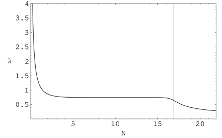
Figure 1: Evolution of $\lambda$ for $n=1$. The vertical line marks the time at $\Omega_{\phi o}=0.7$ with $N_{total}=17.04$.

The development of $\Omega_{\phi}$ can be in agreement with the restriction of the nucleosynthesis stage $\Omega_{\phi}(\mathrm{NS})<0.1$ [15] as well as with the observational result $\Omega_{\phi o}=0.7$ (the subscript $o$ refers to present day quantities). This can be observed in Figure 2, together with the evolution of $w_{\phi}$ which fulfills the condition $w_{\phi o}<-2/3$ [3].

The analysis of inverse power potentials has been extensively studied [4]-[12]. However, the analysis has not been specific enough to determine their viability to describe the late evolution of our universe. In Steinhardt et al. [4] the scalar field was required to track before present day and this imposes a constraint on $n$ to be larger than 5 and thus ruling this models out since they have $w_{\phi o}>-0.52$ in contradiction to SN1a data. The models we will concentrate on are, therefore, models with $n<5$ where $\phi$ has not reached its tracker value.

For future reference we give now the scaling value of $\phi$ [4]

$$\phi_{sc} = \phi_{i}+\sqrt{6\Omega_{\phi i}}\hskip 113.81102ptfor\;\;\Omega_{\phi i}<1/2$$

$$\phi_{sc} = \phi_{i}+\sqrt{6}\left(\frac{1}{\sqrt{2}}+\frac{1}{2}Log[\frac{\Omega_{\phi i}}{1-\Omega_{\phi i}}]\right)\hskip 28.45274ptfor\;\;\Omega_{\phi i}>1/2$$ (5)

The scaling value only depends on the initial conditions $\Omega_{\phi i}$, it is independent on $\Lambda_{c},H_{i}$, since $\phi_{i}\ll 1$. The tracker value of $w$ is given by [4]

$$w_{tr}=-1+\frac{n}{2+n}(w_{\gamma}+1)$$ (6)

and it is an attractor solution valid for large $n$, when $\phi$ is already tracking. In the tracker limit [4], i.e. $n=5$, from eq.(6) one has $w_{tr}=-0.28$ but the value obtained numerically is only $w_{o}=-0.52$ for $\Omega_{\phi i}>0.25$. For smaller $n$ the discrepancy is even worse since the scalar field has not reached its tracker value, obtained from eqs.(6) and (15),

$$\phi_{tr}=\sqrt{\frac{n(2+n)\Omega_{\phi o}}{3}},$$ (7)

which is larger than $\phi_{sc}$ if $\Omega_{\phi i}<\frac{n(2+n)}{18}\Omega_{\phi o}$.

A semi-analytic approach is useful to study some properties of the differential equation system given by eqs.(3). To do this we initially consider only the terms that are proportional to $\lambda$, since $\lambda\gg 1$, then we follow the evolution of $x$, $y$ and $H$ so every period has a characteristic set of simplified differential equations. The parameter $\Omega_{\phi}$ is adequate to divide the process into four periods, the first one being a short lapse in which $\Omega_{\phi}=constant$, easier to recognize in Figure 3; the second is defined from the fall of this parameter to negligible values; the third is the so-called scaling period and in the fourth $\Omega_{\phi}$ is again considerable, eventually reaching the value $0.7$.

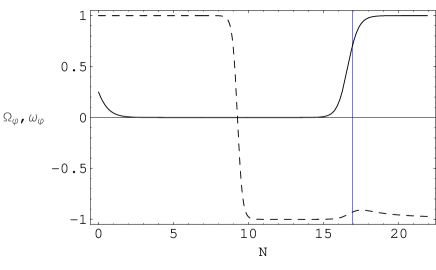
Figure 2: Evolution of $\Omega_{\phi}$ (solid curve) and $w_{\phi}$ (dashed curve) for $n=1$. The vertical line marks the time at $\Omega_{\phi o}=0.7$.

The phase plane $x-y$ provides an illustrative approach, useful for the analysis. We see, from Figure 3, that the system follows, at first, a circular path with $\equiv x^{2}+y^{2}=\Omega_{\phi i}$ constant and ends up with $x^{2}\simeq\Omega_{\phi i}\gg y^{2}$. Then, $x$ and $y$ decrease to negligible values, this situation prevails all along the scaling period. Finally, a growth in both parameters causes $\Omega_{\phi}$ to reach what we set as the final value $0.7$, preferred by observational results. From the restriction over the equation of state parameter, $w_{\phi}<-2/3$ and the observational range for $\Omega_{\phi o}=0.7\pm 0.1$, we can define a region limited by the expressions: $y^{2}=\frac{1-w_{\phi}}{1+w_{\phi}}x^{2}$ with $w_{\phi}=-2/3$ and $y^{2}=\Omega_{\phi o}-x^{2}$ with $0.6\leq\Omega_{\phi o}\leq 0.8$.

Figure 3: Phase plane $x-y$ for $n=1$. Starting point is $(0,0.5)$. The region defined by $w_{\phi o}<-2/3$ and $\Omega_{\phi o}=0.7\pm 0.1$ is shown.

The minimal value $y_{min}$ of $y$ after its initial steep descent is given from eq.(3) with $y_{N}=0,x^{2}\simeq\Omega_{\phi i}$ and $\lambda x\sqrt{3/2}=-H_{N}/H=3\gamma_{\gamma}/2$ by

$$y_{min} = y_{i}\left(\frac{\Lambda_{c}}{\phi_{min}}\right)^{\frac{n}{2}}$$

$$\phi_{min} = \frac{n}{4}\sqrt{6\Omega_{\phi i}}$$ (8)

and we have approximated $H_{min}\simeq H_{i}$ in eq.(3). Shortly after $y$ reaches its minimum value the scaling period begins. In this period we neglect the term proportional to $\lambda$ in eqs.(3) to find:

$$\frac{y_{N}}{y}=-\frac{H_{N}}{N}$$ (9)

which leads to $yH=H_{min}y_{min}\simeq H_{i}y_{min}$. Notice that the dependence of $\lambda$ from $y$ and $H$ is given by $\lambda=A\ (yH)^{2/n}$ with $A$ a constant, therefore from eq.(9) we have $\lambda=constant$ (i.e. $\phi=constant$) during all of the scaling period, this holds for any $n$. Furthermore, we may neglect squared terms on $x$ and $y$ in the third equation of system (3), since they are small, to get the expressions

$$H = H_{i}e^{-\frac{3}{2}\gamma_{\gamma}N}$$

$$y = y_{min}e^{\frac{3}{2}\gamma_{\gamma}N}$$ (10)

The quantity $y$ has an increasing exponencial form for almost all of the process, so the duration of this regime can be seen as the total time (see Figure 4). Now, in order to calculate the number of e-folds from the initial value to present day we consider equation (3) to end up with:

$$N_{total}=\frac{2}{3}\ln[\frac{y_{o}}{y_{min}}]$$ (11)

with $y_{min}$ given by eq.(3) and $y_{o}\simeq 0.8$ (to have $\Omega_{\phi o}=.7,w_{\phi o}<-2/3$. The evolution of $\ln(x)$, $\ln(y)$ and $\ln(H)$ as a function of $N$ is seen on Figure (4).

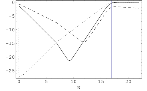
Figure 4: Evolution for $n=1$ of $ln(x)$, $ln(y)$ and $ln(\Omega_{\phi})$ (dashed, dotted and solid lines, respectively). The vertical line marks the time at $\Omega_{\phi o}=0.7$.

If we consider eqs.(3) and assume that the end of the scaling period is very close to today we get an approximated equation $y_{o}H_{o}\simeq H_{min}y_{min}=H_{i}y_{i}(\phi_{i}/\phi_{min})$. This, together with eq.(3) and the definition of $y^{2}_{i}=c^{2}\Lambda_{c}^{4}/3H^{2}_{i}$ establishes an expression for $\Lambda_{c}$, the energy scale at which the scalar field appears, in terms of $y_{o}$, $H_{o}$:

$$\Lambda_{c}=\left(\frac{3y_{o}^{2}H_{o}^{2}}{c^{2}}\right)^{\frac{1}{4+n}}\phi_{min}^{\frac{n}{4+n}}$$ (12)

and $\phi_{min}=\frac{n}{4}\sqrt{6\Omega_{\phi i}}$. The later expression is a semi-analytic calculation of the initial energy scale of a specific model. Finally, the value $y_{o}$ is set to be of the order of $0.8$ to satisfy simultaneously $\Omega_{\phi o}=0.7$ and condition $w_{\phi o}<-2/3$.

Of course, we could have guessed expression (12) using the definition of $y_{o}^{2}=\frac{c^{2}\Lambda_{c}^{4+n}}{3H_{o}^{2}}\phi_{o}^{-n}$ to give [7]

$$\Lambda_{c}=\left(\frac{3H_{o}^{2}y_{o}^{2}\phi_{o}^{n}}{c^{2}}\right)^{\frac{1}{4+n}}\simeq H_{o}^{\frac{2}{4+n}}$$ (13)

and the last equality holds approximately since we expect to have $y_{o},\phi_{o}$ of the order of one.

Now, we wish to determine the value of $w_{\phi o},y_{o}$ and $\phi_{o}$. We use the differential equation for $\gamma_{\phi}=w_{\phi}+1$ and $\Omega_{\phi}$ [18]

$$(\gamma_{\phi})_{N} = 3\gamma_{\phi}(2-\gamma_{\phi})\left(\lambda\sqrt{\frac{\Omega_{\phi o}}{3\gamma_{\phi}}}-1\right)$$

$$(\Omega_{\phi})_{N} = 3(\gamma_{\gamma}-\gamma_{\phi})\Omega_{\phi}(1-\Omega_{\phi}).$$ (14)

We see that $\gamma_{\phi}$ is extremized at $w_{\phi}=\gamma_{\phi}-1=-1,1$ and at $w_{\phi}=-1+\frac{\lambda^{2}\Omega_{\phi}}{3}=-1+\frac{n^{2}\Omega_{\phi}}{3\phi^{2}}$. We have checked that the value of $w_{\phi}$ at the maximum evaluated at $\phi_{o}$ is a very good approximation (within $5\%$ of the numerical value)

$$w_{\phi o}=-1+\frac{n^{2}\Omega_{\phi o}}{3\phi_{o}^{2}}.$$ (15)

Eq. (15) should be compared with [7] which differs by the factor of $\Omega_{\phi o}\simeq 0.7$. Of course, if we do not have the exact value of $\phi_{o}$ eq.(15) is not very useful. In order to determine $\phi_{o}$ we evolve eqs.(3) and eq.(3) from present day values to the scaling regime where $w_{\phi sc}\simeq-1$ and $x_{sc}^{2}\ll y_{sc}^{2}\simeq\Omega_{\phi sc}$ with the condition $\Omega_{\phi o}=0.7$. This evolution is model independent if $0\leq w_{\phi}+1\ll 1$ [18] and from the definition of $y^{2}$ we have

$$\frac{c^{2}}{3}\Lambda_{c}^{4+n}=y_{o}^{2}H_{o}^{2}\phi_{o}^{n}=y_{sc}^{2}H_{sc}^{2}\phi_{sc}^{n}$$ (16)

and we obtain

$$y_{o}^{2}\phi^{n}_{o}=\frac{y_{sc}^{2}H_{sc}^{2}\phi_{sc}^{n}}{H_{o}^{2}}=\phi^{n}_{sc}\Omega_{\phi o}$$ (17)

where we have used $H_{N}/H\simeq-3(1-\Omega_{\phi})/2,H_{sc}^{2}/H^{2}_{o}=(1-\Omega_{\phi o})e^{3\Delta N}$ and $y^{2}_{sc}\simeq\Omega_{\phi}=\Omega_{\phi o}e^{-3\Delta N}/(1-\Omega_{\phi o}+\Omega_{\phi o}e^{-3\Delta N}),\;\;\Delta N\gg 1$ [18]. Using eqs.(17), (15) and (3) we can solve easily for $\phi_{o}$ and/or $y_{o}$ in terms of $\Omega_{\phi o},n$ and $\Omega_{\phi i}$ (via $\phi_{sc}$),

$$\phi_{o}^{2}-\phi_{sc}^{n}\phi_{o}^{2-n}-\frac{n^{2}}{6}\Omega_{\phi o}=0$$ (18)

or equivalently

$$y_{o}^{2}\left(\frac{n^{2}\Omega_{\phi o}^{2}}{6(\Omega_{\phi o}-y_{o}^{2})}\right)^{\frac{n}{2}}=\phi_{sc}^{n}\Omega_{\phi o}.$$ (19)

In order to analytically solve eqs.(18,19) we need to fix the value of $n$ and we can determine $w_{\phi o}$ by putting the solution of (18) into eq.(15). Eq.(18) can be rewritten as $\phi_{o}=\phi_{sc}(1-n^{2}\Omega_{\phi o}/6\phi_{o}^{2})^{-1/n}$ and we see that $\phi_{o}>\phi_{sc}$ and $\phi_{o}>n\sqrt{\Omega_{\phi o}/6}$ and we see that $\phi_{o}$ is of the order of 1 ($\Omega_{\phi o}\sim.7$) regardless of the initial conditions. However, the exact value does indeed depend on the initial conditions but for any initial conditions we will have $-1\leq w_{\phi o}\leq w_{tr}$.

If $\gamma_{\phi o}=n^{2}\Omega_{\phi o}/6\phi_{o}^{2}\ll 1$ one has $\phi_{o}\simeq\phi_{sc}$ and for the simple cases of $n=1,2$ and $4$ we can solve explicitly for $\phi_{o}$ and we find $\phi_{o}|_{n=1}=\phi_{sc}/2+\sqrt{9\phi_{sc}^{2}+6\Omega_{\phi o}}/6,\;y^{2}_{o}|_{n=1}=\phi_{sc}(-3\phi_{sc}+\sqrt{9\phi_{sc}^{2}+6\Omega_{\phi o}},\;)$ $\phi_{o}|_{n=2}=\sqrt{\phi_{sc}^{2}+2\Omega_{\phi o}/3},\;y^{2}_{o}|_{n=2}=3\phi_{sc}^{2}\Omega_{\phi o}/(3\phi_{sc}^{2}+2\Omega_{\phi o})$ and $\phi_{o}|_{n=4}=\sqrt{4\Omega_{\phi o}/3+\sqrt{9\phi_{sc}^{2}+16\Omega_{\phi o}}/3},\;$ $y^{2}_{o}|_{n=4}=\Omega_{\phi o}-8\Omega_{\phi o}^{2}/(4\Omega_{\phi o}+\sqrt{9\phi_{sc}^{2}+16\Omega_{\phi o}})$, respectively. Notice that the value of $\phi_{o},w_{\phi o}$ at $\Omega_{\phi o}=0.7$ does not depend on $H_{i}$ or $H_{o}$ and it only depends on $\Omega_{\phi i}$ (through $\phi_{sc}$) and $n$.

We show in Figure 5 how $w_{\phi o}$ varies for different initial conditions $\Omega_{\phi i}$ with $n=18/7\simeq 2.57$ fixed. We see that for larger $\Omega_{\phi i}$ we end up with a smaller $w_{\phi o}$ and this is a generic result as can be seen from eqs.(18),(3) and (15) since for larger $\Omega_{\phi i}$ one has a larger $\phi_{sc}$, $\phi_{o}$ and therefore a smaller $w_{\phi o}$. This can be seen also from Figure 6 where for a small $\Omega_{\phi i}$ a plateau arises in $w_{\phi}$ (the field $\phi$ has already reached its tracker value by present day). From eqs.(15),(18) we notice that for smaller $n$ one gets a smaller $w_{\phi o}$ (see Figure 7).

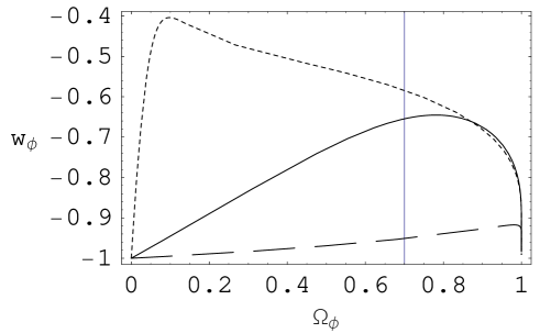
Figure 5: Variations on $\Omega_{\phi i}$ lead to different physical situations given by $w_{\phi o}$. We have taken $\Omega_{\phi i}=0.9,0.25,10^{-10}$ dashed, solid and dotted lines, respectively. The vertical line marks the time at $\Omega_{\phi o}=0.7$.

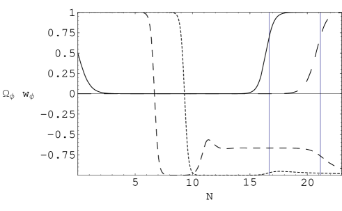
Figure 6: Evolution of $\Omega_{\phi}$ and $w_{\phi}$ for $n=1$. Parameter $\Omega_{\phi}$ evolves in a similar way for $\Omega_{\phi i}=0.25$ (solid line) and $\Omega_{\phi i}=10^{-10}$ (long-dashed line), varying only in the total time, $N_{total}=16.7$ or $21.1$ in the previous order. A discrepancy between the two cases at $\Omega_{\phi o}=.7$ is seen for parameter $w_{\phi}$ because it has, for $\Omega_{\phi i}=0.25$ a local maximum with $w_{\phi o}=-0.93$ (dotted line) while for $\Omega_{\phi i}=10^{-10}$ (short-dashed line) a plateau appears with $w_{\phi o}=-0.76$. The vertical lines mark the time at $\Omega_{\phi o}=0.7$.

3.1 Initial Conditions

It is well known that inverse power law potential lead to attractor solutions [4] and are therefore independent of the initial conditions (one has 100 orders of magnitud range for $\Omega_{\phi i}$). However, as pointed out by Steinhardt et al, this is only the case for $n>5$, for smaller values of $n$ the field $\phi$ has not necessarily reached its tracker value at present time. However, even though in these cases the present day quantities depend on the initial conditions there is no fine tuning problem since we can vary the initial conditions on a wide range of values (i.e. 45%) and the end results are still physical acceptable.

The differential equations given in eqs.(3) depend on values of $x,y,\lambda=n/\phi$ but they do not depend on the absolute value of H, i.e. we have the same evolution for $x,y,H$ as for $x,y,H^{\prime}=kH$ where $k$ is an arbitrary constant. This scaling freedom allow us to set the normalization of $H$ as we wish and in particular to have $\Omega_{\phi o}=0.7$ at $H=H_{o}$ for any values of the initial conditions $x_{i},y_{i}$. This implies that we can have a quintessence model for arbitrary initial conditions. Once $H_{o}$ is fixed we get $\Lambda_{c}\simeq H_{o}^{2/(4+n)}$ (eq.(20)) and $H_{i}=c\Lambda^{2}_{c}/y_{i}$ (from the definition of $y_{i}$). One of the main difference with the tracker solution is that $w_{\phi o}$ or $\phi_{o}$ do not have the same values in all cases but depend on $\Omega_{\phi i}$ as can be seen from eqs.(15) and (18). However, the dependence on $\Omega_{\phi i}$ is mild since for example for $n=1$ one has that $\phi_{o}$ only depends as $\sqrt{\Omega_{\phi i}}$. For this reason once $H_{o}$ and $\Omega_{\phi i}$ are fixed we still have a wide range of values of $\Omega_{\phi i}$ giving the correct phenomenology, i.e. $\Delta\Omega_{\phi i}=45\%$. For $\Omega_{\phi i}\ll 1$, i.e. $y_{i}=c\Lambda_{c}/H_{i}\ll 1$, with a fixed $\Lambda_{c}$ one has a larger $H_{i}$ and the time of expansion up to present day is also larger. In this case it is posible that the $\phi$ field has already reached its tracker value, even for $n<5$, and we would have $w_{\phi o}=w_{tr}=-2/(2+n)$. Indeed, it can be seen from eq.(18) that a $\Omega_{\phi i}\ll 1$ renders a $\phi_{o}\sim n\sqrt{\Omega_{\phi o}/6}$ and independent of the initial conditions. For any initial conditions we will end up with $-1\leq w_{\phi o}\leq w_{tr}$.

4 Quintessence Restriction on $n$

Before analyzing the quintessence restriction imposed on $n$ we would like to comment on the value of $c$ in the potential eq.(1). It can take different values with different physical interpretations.

For simplicity of arguments let us assume that we have no kinetic energy at the beginning and that $\rho_{\phi i}=V_{i}=c^{2}\Lambda_{c}^{4}$. The initial energy density is $\Omega_{\phi i}=\rho_{\phi i}/\rho_{c}$. Taking $\rho_{\phi i}=c^{2}\Lambda_{c}^{4}$, with $c=2\nu$, and $\rho_{c}=E^{4}$ we have that the initial energy density is given by $\Omega_{\phi i}=(2\nu)^{2}(\Lambda_{c}/E)^{4}$. In this case we see that the initial energy density depends on the ratio between the condensation scale $\Lambda_{c}$ and the critical energy density $E=\rho_{c}^{1/4}$.

Another possibility is to take $\rho_{\phi i}=g_{\phi}T^{4}$ and $\rho_{c}=g_{Tot}T^{4}$ where $g_{Tot},g_{\phi}$ are the total and quintessence number of degrees of freedom, respectively, at a temperature $T$. In this case we have $\Omega_{\phi i}=g_{\phi}/g_{Tot}$ and it only depends on the ratio of quintessence and total degrees of freedom and not on the energy scales. The condensation scale is then $\Lambda_{c}=(g_{\phi}/c^{2})^{1/4}T$ and $\rho_{\phi i}=g_{\phi}T^{4}=c^{2}\Lambda_{c}^{4}=V_{i}$.

Let us now, study the restrictions to the values of $n$. In both cases, mentioned above, we get similar restrictions so we will only consider the first one.

For a fixed $n$ we take the following conditions: $h_{o}$ must be in the range $.7\pm.1$ and $\Omega_{\phi o}$ must belong to the interval $0.6-0.8$. We can restrict $n$ according to different physical arguments. These restrictions are encountered while solving numerically the differential system settled by equations (3), the first restriction comes from the observational value of the relevant parameter $w_{\phi o}$. The limit $w_{\phi o}<-2/3$ can be translated to $w_{eff}<-0.7$ [3]. Notice that in this potentials $w_{eff}<w_{\phi o}$ contrary to the general arguments [4] and the reason is that $w_{\phi}$ is still growing by today. From this analysis we find that, in order to fulfill the $w_{eff}$ condition, $n$ must be smaller than $2.74$ as shown in Figure 7 for $\Omega_{\phi i}=0.25$. The value of $w_{\phi o}$ depends not only on $n$ but also on $\Omega_{\phi i}$ and it decreases with increasing $\Omega_{\phi i}$. If we fix $n$ and increase $\Omega_{\phi i}$ we find that examples originally discarded by the $w_{eff}<-0.7$ restriction now enter the physically permitted group. The example with $n=3$ is depicted in Figure 8. An equipartition value of $\Omega_{\phi i}$ is 0.25 but if we allow $\Omega_{\phi i}$ to be as large as 0.75 than the restriction on $n$ is only $n<5.2$.

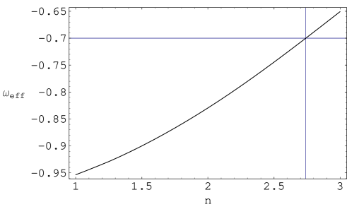
Figure 7: Restriction over $n$ from $w_{eff}<-0.7$ with $c=1$ and $\Omega_{\phi i}=0.35$)

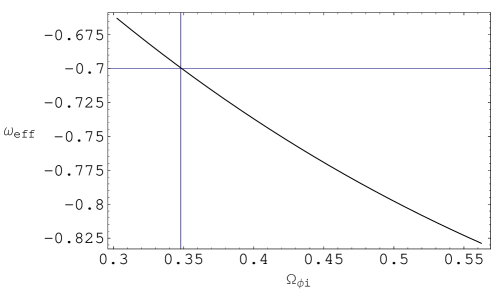
Figure 8: Restriction $w_{eff}<-0.7$ avoided by increasing $\Omega_{\phi i}$ with $n=3$ ($c=1$)

Other restriction comes from big bang nucleosynthesis (NS) results that require $\Omega_{\phi}(\mathrm{NS})<0.1$ at the energy scale range of NS: $0.1-10\ \mathrm{MeV}$ [15]. To account for this we have to either consider $\Omega_{\phi i}<0.1$ or, for example, if $\Omega_{\phi i}=0.25$ we must take out $1.2<n<2.1$ because for this range the initial value $H_{i}$ lies within the range of values of $H_{\mathrm{NS}}$. For all the values of $n$ allowed by $w_{eff}$ and NS restrictions, a variation of $45\%$ on $\Omega_{\phi i}$ can be performed without disturbing the permanence into the observed ranges of $H_{o}$ and $\Omega_{\phi o}$.

5 Unification of Gauge Couplings Constants

The condensation scale $\Lambda_{c}$ used in eq.(1) is from an elementary particle point of view an arbitrary scale that sets the energy scale of the phase transition. However, if the inverse power potential eq.(2) is obtained from a non-abelian asymptotically free gauge group then we can relate the condensation scale $\Lambda_{c}$ to other energy scales using the renormalization group equation. The one-loop evolution of the gauge coupling constant for an $SU(N_{c})$ gauge group with $N_{f}$ chiral fields gives a condensation scale (strong coupling $g^{-2}\ll 1$)

$$\Lambda_{c}=\Lambda_{x}e^{-\frac{1}{2b_{o}g^{2}_{x}}}$$ (20)

where $b_{o}=(3N_{c}-N_{f})/16\pi^{2}$ is the one-loop beta function and $\Lambda_{x},g_{x}$ are arbitrary energy scale and coupling constant, respectively, which include high energy scale where the original chiral fields $Q$ are weakly coupled.

It is well known that the gauge coupling constants of the standard model get unified at a energy scale $\Lambda_{gut}\simeq 10^{16}\mathrm{GeV}$ with a coupling constant $g_{gut}\simeq\sqrt{4\pi/25.7}$.

We want to impose to our model gauge coupling unification, i.e. the coupling of the gauge group responsible for quintessence should be unified at $\Lambda_{gut}$ with the standard model gauge groups [10]. In this case we require $\Lambda_{x},g_{x}$ in eq.(20) to take the values $\Lambda_{x}=\Lambda_{gut},g_{x}=g_{gut}$ and we have $\Lambda_{c}=\Lambda_{gut}exp[-1/2b_{o}g^{2}_{gut}]$. This is not a necessary condition but opens the possibility of thinking of the model as coming from string theory after compactifying the extra dimensions or on a Grand Unification Scheme where all gauge coupling constants are unified.

Of course, not all values of $N_{c},N_{f}$ will give an acceptable phenomenology. This is because the cosmological evolution of $\phi$ and the gauge coupling unification set independent constrains on the condensation scale $\Lambda_{c}$ and on $N_{c},N_{f}$. From a cosmological point of view $\Lambda_{c}$ depends on the inverse power $n$ (see eq.(13)), which is a function of $N_{c},N_{f}$, and from gauge unification $\Lambda_{c}$ depends also on $N_{c},N_{f}$ through $b_{o}$ (see eq.(20)). These two constrains reduce drastically the allowed values of $N_{c},N_{f}$ and we also require $N_{f}\geq 1$ and $N_{c}\geq 2$ to be integers.

In table 1 we give the different values of $N_{c},N_{f},\nu$ for which we have gauge coupling unification. We can see that there are only a small number of possible models (11). The first five models have an $N_{f}$ which differs form an integer by less than $0.05$ while the other 6 models differ at most by $0.10$. All other combinations of $N_{c},N_{f},\nu$ have a larger discrepancy and do not lead to $\Lambda_{c}=\Lambda_{u}$. If we further constrain the models to agree with the cosmological observations (i.e. $w_{\phi o}<-0.7$ requiring $n<5$) we are left with only 4 models (number 1,2,3,11 of table 1). All of these 4 models have $n<2$ and the quantum corrections to the Kahler potential are, therefore, not dangerous. Notice as well that only two models (4,9) have $\nu=N_{f}$ and in both cases $n>12$.

Num	$N_{c}$	$N_{f}$	$\nu$	$n$	$\Lambda_{c}$(GeV)
1	3	5.98	1	0.66	$6\times 10^{-8}$
2	6	14.97	3	0.66	$6.9\times 10^{-8}$
3	7	18.05	4	0.55	$1.6\times 10^{-8}$
4	8	5.97	5.97	13.83	$1.3\times 10^{12}$
5	8	6.96	3	13.55	$7.6\times 10^{11}$
6	3	1.90	1	5.66	$1.3\times 10^{6}$
7	5	3.91	2	9.38	$4.7\times 10^{9}$
8	6	5.09	2	10.85	$3.7\times 10^{10}$
9	7	5.08	5.08	12.64	$3.9\times 10^{11}$
10	8	20.90	4	6.75	$2.4\times 10^{-7}$
11	8	21.10	5	0.47	$5.7\times 10^{-9}$

Table 1: Models with $\Lambda_{c}=\Lambda_{u}$. The first 5 have $\Delta N_{f}<0.05$ while the other 6 have $\Delta N_{f}<0.10$ discrepancy from an integer

$n$	$H_{i}$ (GeV)	$\rho_{\phi i}^{1/4}$(GeV)	$\Lambda_{c}$ (GeV)	$w_{\phi o}$	$w_{eff}$	$N_{total}$
$1/2$	$1.33\times 10^{-35}$	$7.48\times 10^{-9}$	$3.74\times 10^{-9}$	$-0.97$	$-0.98$	10.72
$2/3$	$1.16\times 10^{-33}$	$6.99\times 10^{-8}$	$3.49\times 10^{-8}$	$-0.97$	$-0.98$	12.96
$1$	$3.46\times 10^{-30}$	$3.82\times 10^{-6}$	$1.91\times 10^{-6}$	$-0.93$	$-0.95$	16.97
$2$	$4.68\times 10^{-22}$	$4.44\times 10^{-2}$	$2.22\times 10^{-2}$	$-0.77$	$-0.83$	26.33
$18/7$	$1.68\times 10^{-18}$	$2.66$	$1.33$	$-0.65$	$-0.73$	30.42
$3$	$3.41\times 10^{-16}$	$37.92$	$18.77$	$-0.57$	$-0.65$	33.07

Table 2: Numerical solutions for different values of $n$ with $c=1$ and $\Omega_{\phi i}=0.25$.

$\Omega_{\phi i}$	$H_{i}$ (GeV)	$\rho_{\phi i}^{1/4}$	$\Lambda_{c}$ (GeV)	$w_{\phi o}$	$w_{eff}$	$N_{total}$
$1\times 10^{-5}$	$5.48\times 10^{-14}$	$480.90$	$19.12$	$-0.55$	$-0.50$	35.69
$0.25$	$3.34\times 10^{-16}$	$37.54$	$18.77$	$-0.57$	$-0.65$	33.07
$0.5$	$2.85\times 10^{-16}$	$34.68$	$20.62$	$-0.76$	$-0.83$	32.88
$0.75$	$3.05\times 10^{-16}$	$35.88$	$23.61$	$-0.88$	$-0.92$	32.75
$0.99$	$5.13\times 10^{-16}$	$46.53$	$32.82$	$-0.97$	$-0.98$	32.20

Table 3: Numerical solutions for different values of $\Omega_{\phi i}$ with $c=1$ and $n=3$.

As an example of a model with gauge coupling unification we have a gauge group $N_{c}=3$ with $N_{f}=6$ and $\nu=1$ which entails a value $n=2/3$ according to $n=2+\frac{4\nu}{N_{c}-N_{f}}=2/3$ [10]. For this model we find, from the numerical solution, a total time $N_{total}=12.96$ which does not superposes on the NS range $19.6-27.2$. The $w_{eff}<-0.7$ restriction is satisfied with $w_{eff}=-0.98$ and the condition from experimental central values $h_{o}=0.7$ and $\Omega_{\phi o}=0.7$ is also fulfilled taking $\Omega_{\phi i}=0.25$. The condensation scale is $\Lambda_{c}=4.2\times 10^{-8}\ \mathrm{GeV}$. A full analysis of this model is presented in [20].

6 Further Examples

We have already given some example in the previous sections. In table 2 and 3 we show the numerical results for different values of $n$ with initial condition $\Omega_{\phi i}=0.25$ and for different initial condition with n=3 fixed, respectively.

Other interesting examples are when $\nu=N_{f}$. The condition $n<2.74$ (for $\Omega_{\phi i}\leq 0.25$) requires $N_{f}/N_{c}<0.15$ and therefore $N_{c}>7$. For $N_{c}=8,N_{f}=1$ one has $n=18/7\simeq 2.57$ and using $\Omega_{\phi i}=0.25$ and one obtains $w_{\phi o}=-0.65,w_{eff}=-0.73,\phi_{o}=2.01,N_{o}=30.3$ and $M_{i}=2.3$ GeV $\Lambda_{c}=1.6$ GeV while for $N_{c}=7,N_{f}=1$ one has $n=8/3,w_{\phi o}=-0.64,w_{eff}=-0.71,\phi_{o}=2.04,N_{o}=30.9,M_{i}=4.2GeV,\Lambda_{c}=3GeV$. However, these models do not have $\Lambda_{c}=\Lambda_{u}$, i.e. they are not unified with the SM gauge groups.

7 Conclusions

We studied negative power potentials and we constrain the initial conditions an the power of the potential to satisfy the SN1a results. For $n$ larger than 5, the scalar field $\phi$ has already reached its tracker value and $w_{\phi o}$ is too large. So, we need to concentrate on potentials with $n<5$ to comply with SN1a results. We gave a semi analytic solution to $w_{\phi o}$ and $\Lambda_{c}$ in terms of $H_{o},\Omega_{\phi i}$ and $n$ and we have solved numerically for some relevant cases. We obtained that $w_{\phi o}$ depends on $\Omega_{\phi i},n$ and it decreases with increasing $\Omega_{\phi i}$ while it becomes smaller for larger $n$. If we assume equipartition initial conditions with $\Omega_{\phi i}\leq 0.25$ than $n$ is constrained to be smaller than $n<2.74$, however, if we allow for $\Omega_{\phi i}=0.75$ the constraint is relaxed to $n<5.2$. We have shown that one can vary the initial conditions up to $45\%$ without spoiling the observational cosmological values at present time. For any initial conditions we will end up with $-1\leq w_{\phi o}\leq w_{tr}$.

We have seen that the negative power potentials can be derived from Affleck’s potential and in order to avoid problems with the Kahler potential one requires $n<2$ which implies that $N_{f}>N_{c}$ and that not all condensate become dynamically (i.e. $\nu\neq N_{f}$). For $\nu=N_{f}$ one needs $N_{f}/N_{c}<0.15$ to have $w_{\phi o}<-2/3$. Furthermore, we have shown that it is possible to have a quintessence model with gauge coupling unification for all gauge groups, Standard Model and the gauge group responsible for quintessence, but the number of models is quite limited (4).

This work was supported in part by CONACYT project 32415-E and DGAPA, UNAM project IN-110200.

References

- [1] A.G. Riess et al., Astron. J. 116 (1998) 1009; S. Perlmutter et al, ApJ 517 (1999) 565; P.M. Garnavich et al, Ap.J 509 (1998) 74.
- [2] P. de Bernardis et al. Nature, (London) 404, (2000) 955, S. Hannany et al.,Astrophys.J.545 (2000) L1-L4
- [3] S. Perlmutter, M. Turner and M. J. White, Phys.Rev.Lett.83:670-673, 1999; T. Saini, S. Raychaudhury, V. Sahni and A.A. Starobinsky, Phys.Rev.Lett.85:1162-1165,2000
- [4] I. Zlatev, L. Wang and P.J. Steinhardt, Phys. Rev. Lett.82 (1999) 8960; Phys. Rev. D59 (1999)123504
- [5] P.J.E. Peebles and B. Ratra, ApJ 325 (1988) L17; Phys. Rev. D37 (1988) 3406
- [6] J.P. Uzan, Phys.Rev.D59:123510,1999
- [7] P. Binetruy, Phys.Rev. D60 (1999) 063502, Int. J.Theor. Phys.39 (2000) 1859
- [8] A. Masiero, M. Pietroni and F. Rosati, Phys. Rev. D61 (2000) 023509
- [9]
- [10] A. de la Macorra and C. Stephan-Otto, Phys. Rev. Lett. 87, (2001) 271301, astro-ph/0106316
- [11] A.R. Liddle and R.J. Scherrer, Phys.Rev. D59, (1999)023509
- [12] A. de la Macorra and G. Piccinelli, Phys. Rev.D61 (2000) 123503
- [13] E.J. Copeland, A. Liddle and D. Wands, Phys. Rev. D57 (1998) 4686
- [14] E.Kolb and M.S Turner,The Early Universe, Edit. Addison Wesley 1990
- [15] K. Freese, F.C. Adams, J.A. Frieman and E. Mottola, Nucl. Phys. B 287 (1987) 797; M. Birkel and S. Sarkar, Astropart. Phys. 6 (1997) 197.
- [16] I. Affleck, M. Dine and N. Seiberg, Nucl. Phys.B256 (1985) 557
- [17] C.P. Burgess, A. de la Macorra, I. Maksymyk and F. Quevedo Phys.Lett.B410 (1997) 181
- [18] A. de la Macorra, Int.J.Mod.Phys.D9 (2000) 661
- [19] U. Amaldi, W. de Boer and H. Furstenau, Phys. Lett.B260 (1991) 447, P.Langacker and M. Luo, Phys. Rev.D44 (1991) 817
- [20] A. de la Macorra hep-ph/0111292