Chandra Imaging of The X-ray Nebula Powered by Pulsar B1509–58

Abstract

We present observations with the Chandra X-ray Observatory of the pulsar wind nebula (PWN) powered by the energetic young pulsar B1509–58. These data confirm the complicated morphology of the system indicated by previous observations, and in addition reveal several new components to the nebula. The overall PWN shows a clear symmetry axis oriented at a position angle $150^{\circ}\pm 5^{\circ}$ (north through east), which we argue corresponds to the pulsar spin axis. We show that a previously identified radio feature matches well with the overall extent of the X-ray PWN, and propose the former as the long-sought radio nebula powered by the pulsar. We further identify a bright collimated feature, at least $4^{\prime}$ long, lying along the nebula’s main symmetry axis; we interpret this feature as a physical outflow from the pulsar, and infer a velocity for this jet $>0.2c$. The lack of any observed counter-jet implies that the pulsar spin axis is inclined at $\sim 30^{\circ}$ to the line-of-sight, contrary to previous estimates made from lower-resolution data. We also identify a variety of compact features close to the pulsar. A pair of semi-circular X-ray arcs lie $17^{\prime\prime}$ and $30^{\prime\prime}$ to the north of the pulsar; the latter arc shows a highly-polarized radio counterpart. We show that these features can be interpreted as ion-compression wisps in a particle-dominated equatorial flow, and use their properties to infer a ratio of electromagnetic to particle energy in pairs at the wind shock $\sigma\sim 0.005$, similar to that seen in the Crab Nebula. We further identify several compact knots seen very close to the pulsar; we use these to infer $\sigma<0.003$ at a separation from the pulsar of 0.1 pc.

1. Introduction

Pulsars and supernova remnants (SNRs) are both believed to be formed in supernova explosions. However, there are still fewer than 20 cases in which convincing associations between a pulsar and a SNR have been established. These few systems provide important information on the properties of pulsars and SNRs, and on the relationship and interaction between them. In particular, in cases where a pulsar is still inside its associated SNR, the high-pressure environment can confine and shock the pulsar’s relativistic wind. This generates synchrotron emission, producing an observable pulsar wind nebula (PWN) which can be used to trace the energy flow away from the pulsar.

For almost 15 years, the Crab Nebula and the Vela SNR were the only SNRs known to be associated with pulsars. A third association only emerged when a 150-ms X-ray, radio and $\gamma$-ray pulsar, PSR B1509–58, was discovered within the SNR G320.4–1.2 (MSH 15–52) (Seward & Harnden Jr. (1982); Manchester, Tuohy, & D’Amico (1982); Ulmer et al. (1993)). The pulsar’s spin-parameters can be used to infer a characteristic age $\tau_{c}=1700$ yr, a spin-down luminosity $\dot{E}=1.8\times 10^{37}$ erg s^-1 and a surface magnetic field $B_{p}=1.5\times 10^{13}$ G (Kaspi et al. (1994)), making it one of the youngest, most energetic and highest-field pulsars known.

SNR G320.4–1.2 has an unusual radio appearance, consisting of two well-separated radio regions (Fig. 1; Gaensler et al. (1999), hereafter G99). While the more southerly of these regions approximates a partial shell, the northern component is bright, centrally concentrated, and has an unusual ring of radio clumps near its center. While it had been previously suggested that G320.4–1.2 consisted of two or three separate SNRs, G99 have used H i absorption measurements to confirm that this source is indeed a single SNR at a distance of $5.2\pm 1.4$ kpc. Assuming standard parameters for the interstellar medium (ISM) and for the supernova explosion, an age of $\sim$6–20 kyr is derived for the SNR, an order of magnitude larger than the 1700 yr implied by the pulsar spin-down (Seward et al. (1983)). One possible explanation for this discrepancy is that the pulsar is much older than it seems (Blandford & Romani (1988); Gvaramadze (2001)), but this requires an unusual spin-down history of which there is no evidence from long-term timing (Kaspi et al. (1994)). A more likely explanation is that the SNR has expanded rapidly into a low-density cavity (Seward et al. (1983)). This model can also explain the unusual SNR morphology, the offset of the pulsar from the SNR’s apparent center, and the faintness of any PWN at radio wavelengths (Bhattacharya (1990); G99). This argument is supported by recent observations of H i emission in the region (Dubner et al. (2002)).

X-ray emission from this system, also displayed in Figure 1, has revealed a different but similarly complicated picture. Apart from a pulsed point-source corresponding to the pulsar itself (Seward & Harnden Jr. (1982)), X-ray emission from the system is dominated by an elongated non-thermal source centered on the pulsar, and an extended thermal source coincident with the northern radio component of the SNR and with the optical nebula RCW 89 (Seward et al. (1983); Trussoni et al. (1996)). Faint diffuse X-rays extend over the entire extent of the radio SNR, and potentially correspond to thermal emission from the SNR blast wave (Trussoni et al. (1996)).

The central non-thermal source has been interpreted as a PWN powered by the pulsar (Seward et al. (1984); Trussoni et al. (1996)). As mentioned above, no radio emission from this PWN has been seen, presumably because of the low density into which the pulsar wind expands (Bhattacharya (1990); G99). High-resolution observations with ROSAT show the X-ray PWN to be significantly collimated to the SE of the pulsar (Fig. 1; Greiveldinger et al. (1995)). Several authors have interpreted this region as corresponding to a jet produced by the pulsar (Tamura et al. (1996); Brazier & Becker (1997)).

Using ROSAT PSPC data, Greiveldinger et al.  (1995) have analyzed the morphology of X-ray emission close to the pulsar, and concluded that the PWN has two components: a large region extending over many arcminutes, and a compact disc of emission of radius $30^{\prime\prime}-45^{\prime\prime}$ centered on the pulsar. Brazier & Becker (1997) considered data taken with the ROSAT HRI. They found no evidence for the two-component PWN proposed by Greiveldinger et al.  (1995), but pointed out that the X-ray emission around the pulsar had a cross-shaped morphology. They interpreted this as indicating that the pulsar powers an equatorial torus, as is also seen in X-rays for the Crab pulsar (Aschenbach & Brinkmann (1975); Hester et al. (1995)). This morphology would imply that the jet (and presumably the pulsar spin axis) lies largely in the plane of the sky, inclined at $\sim 70^{\circ}$ from the line-of-sight.

An interpretation for the thermal X-ray source $\sim 6^{\prime}$ to the north of the pulsar is unclear. It has been repeatedly proposed that this region represents an interaction between a collimated outflow from the pulsar and the surrounding SNR (Seward et al. (1983); Manchester & Durdin (1983); Manchester (1987); Brazier & Becker (1997)). Tamura et al.  (1996) showed evidence for a bridge of non-thermal emission connecting the pulsar to the thermal X-ray emission to the north, but it remained uncertain as to whether this was the direct counterpart to the SE jet-like feature. At high spatial resolution, a collection of X-ray clumps is seen at the center of the northern X-ray region, the morphologies and positions of which closely match those of clumps seen at radio wavelengths (Brazier & Becker (1997); G99). It has not been established whether the proposed pulsar outflow powers the entire RCW 89 region (Tamura et al. (1996)) or just the central collection of clumps (G99). But in either case, the evidence for interaction provides a convincing argument that the pulsar and SNR are physically associated.

Clearly PSR B1509–58 and SNR G320.4–1.2 provide an important example of the interaction between a pulsar and its environment. Accordingly, we have obtained sensitive high-resolution observations of this system with the Chandra X-ray Observatory. These data provide the opportunity to clarify the nature of the emission close to the pulsar, to determine the overall structure of the PWN, and to further investigate the apparent interaction between the pulsar and its surrounding SNR. In §2 we describe our observations, in §3 we describe the resulting images and spectra, and in §4 we discuss and interpret these results.

2. Observations and Analysis

G320.4–1.2 was observed on 2000 Aug 14 (ObsID 754) with the Advanced CCD Imaging Spectrometer (ACIS) aboard the Chandra X-ray Observatory (Weisskopf et al. 2000b ). ACIS is an array of ten 1024$\times$1024-pixel CCDs fabricated by MIT Lincoln Laboratory. These X-ray sensitive devices have large detection efficiency (10$-$90%) and moderate energy resolution (10$-$50) over a 0.2–10.0 keV passband. Coupled with the 10-m optics of Chandra, the CCDs have a scale of $0\farcs 492$ per pixel, well-matched to the on-axis point-spread function (FWHM $\lesssim 1^{\prime\prime}$). ACIS and its calibration are discussed in detail by Burke et al.  (1997) and Bautz et al.  (1998).

A single exposure of length 20 ks was made in the standard “Timed Exposure” mode. The data discussed here were recorded from the four CCDs of the ACIS-I array. After standard processing had been carried out at the Chandra Science Center (ASCDS version number R4CU5UPD14.1), we analyzed the resultant events list using CIAO v2.1.3. We first applied the observation-specific list of bad pixels to the data, and then corrected for the $\sim 1^{\prime\prime}$ offset present in ACIS-I observations. After removing small intervals in which data were not recorded, the final exposure time for this observation was 19039 s.

The effective area of the detector is a function of both the energy of incident photons and their position on the sky. To generate an exposure-corrected image, we computed exposure maps at five energies: 0.5, 1.5, 3.0, 5.0 and 7.0 keV. We also computed images of the counts per pixel in the five separate energy bands 0.3–0.8, 0.8–2.0, 2.0–4.0, 4.0–6.0 and 6.0–8.0 keV. For each energy band, we divided the map of raw counts by the exposure map corresponding to that band, and then normalized by the exposure time to produce a final image with units of photons cm^-2 s^-1.

For compact sources of emission ($\leq 5^{\prime\prime}$ in extent), spectra were extracted from the data using the psextract script within CIAO, using a small extraction region immediately surrounding the source of interest. For extended sources we made use of v1.08 of the calcrmf and calcarf routines provided by Alexey Vikhlinin, which generate the response matrix and effective area for a region of the CCD by computing an appropriately weighted mean over small sub-regions. In all cases, the resulting spectra were rebinned to ensure a minimum of 15 counts per spectral channel. The background spectrum for each region was measured by considering an annular region surrounding the source of interest. Subsequent spectral analysis was carried out using XSPEC v11.0.1.

3. Results

3.1. Imaging

An exposure-corrected and smoothed image in the energy range 0.3–8.0 keV, encompassing the entire field-of-view of the ACIS-I array, is shown in Figure 2. The central region is shown on a logarithmic scale in the subpanel at lower-right. Count rates and surface brightnesses for various features (marked in Fig. 2 and discussed below) are given in Table 1.

Marked in Figure 2 as feature A, PSR B1509–58 is clearly detected as a bright source near the center of the field-of-view. The extent of this source is consistent with the point-spread function of the telescope. The pulsar’s X-ray position is measured to be (J2000) RA $15^{\rm h}13^{\rm m}55\farcs 64$, Dec $-59^{\circ}08^{\prime}09\farcs 2$, with an uncertainty of $\pm 0\farcs 5$ in each coordinate. This differs by several arcsec from previous X-ray measurements of the pulsar position (Seward et al. (1984); Brazier & Becker (1997)), but is in excellent agreement with positions measured from radio timing and imaging (Kaspi et al. (1994); G99).

Because the pulsar is so bright, a significant number of counts from it strike the detector during the 41 ms per 3.2-sec frame during which the CCD is read out. This produces a faint trail of emission, marked as feature B, which runs through the pulsar and parallel to the north/south edge of the array (i.e. along the read-out direction).

The morphology of the surrounding X-ray emission as imaged with Chandra is consistent with that seen by ROSAT and ASCA at lower spatial resolution. In particular, we confirm the diffuse nebula seen extending $\sim 6^{\prime}$ NW/SE of the pulsar (Greiveldinger et al. (1995); Trussoni et al. (1996); Tamura et al. (1996)), and the collection of X-ray clumps coincident with the H$\alpha$ nebula RCW 89 (Brazier & Becker (1997)). Most of the nebula is elongated along a position angle $150^{\circ}\pm 5^{\circ}$ (N through E). In all future discussion, we consider this orientation to define the main axis of the system.

To the SE of the pulsar and superimposed on the diffuse nebular emission is a jet-like X-ray feature, denoted as feature C in Figure 2. Close to the pulsar, feature C is aligned with the main nebular axis, but at a distance $\sim 2^{\prime}$ from the pulsar it curves around to the east, before fading abruptly at a separation of $\sim 4^{\prime}$ from the pulsar. This feature is resolved and is approximately $10^{\prime\prime}$ wide.

In Figure 3 we show a comparison between our Chandra data and 1.4-GHz radio observations taken with the Australia Telescope Compact Array (ATCA; G99). There is a good match between the morphologies of the X-ray PWN and the radio “tongue” reported in previous observations (Manchester & Durdin (1983); G99), the radio extent being somewhat larger than the X-ray nebula. Furthermore, it is clear that feature C corresponds to a trough of reduced radio emission, confirming a similar correspondence seen when comparing ATCA and ROSAT observations (G99).

We see no obvious counterpart in Figure 2 to feature C on the other side of the pulsar. Rather, to the NW of the pulsar there is an elongated region of reduced emission, beginning $3^{\prime}$ from the pulsar and extending for $3^{\prime}$ along the nebular axis. We refer to this as feature D. The width of this fainter region is a function of distance from the pulsar: at its end nearest the pulsar, this feature is $\sim 25^{\prime\prime}$ across, but it widens to $75^{\prime\prime}$ at its NW end.

Approximately $30^{\prime\prime}$ to the north of the pulsar is feature E, a semi-circular arc of emission, approximately centered on the pulsar. This arc is resolved by Chandra, with approximate width $15^{\prime\prime}$. The arc is brightest immediately to the north of the pulsar, fading slowly to the east and more rapidly to the west. Along the main symmetry axis defined above, the pulsar is separated from the inner edge of this arc by $30^{\prime\prime}$, and from the outer edge by $45^{\prime\prime}$.

We have re-examined the 1.4- and 5-GHz images presented by G99 to look for a radio counterpart to feature E. In total intensity, this region is confused by emission from RCW 89 (see Fig. 3), and we can identify no specific radio feature which might be associated. However, we have re-analyzed the 5-GHz polarization data of G99, deconvolving the data with a new maximum entropy algorithm specifically designed for polarimetric observations (PMOSMEM; Sault, Bock, & Duncan (1999)). In Figure 4 we compare the resulting distribution of linear polarization to the X-ray emission in the same region. While there is generally a high level of polarization from the area, there is a clear enhancement of the linearly polarized signal in an arc $\sim 30^{\prime\prime}$ to the north of the pulsar, whose extent and morphology match closely that of the X-ray emission from feature E.

Returning to Figure 2, it can be seen that the perimeter of the overall diffuse nebula is reasonably well-defined. This is particularly the case to the west of the pulsar, where feature F, a sharp-edged protuberance, extends $\sim 2^{\prime}$ to the WNW of the main body of the nebula. A similar, but smaller and less well-defined feature may exist on the opposite side of the nebular symmetry axis.

Figure 5 shows the X-ray emission immediately surrounding the pulsar at the full resolution of the data. In increasing order of distance from the pulsar (marked as A), we point out various features of interest:

1. Approximately $3^{\prime\prime}$ to the NW of the pulsar, a small clump of emission $\sim 3^{\prime\prime}$ across. This feature is too far from the pulsar and too irregular in appearance to be due to asymmetries in the wings of the point-spread function (cf. Pavlov et al. (2001)). The count rate from this source is approximately constant over the observation, so it cannot result from pulsar photons assigned to the wrong location on the sky (as might result from errors in the aspect solution).

2. Lying $8^{\prime\prime}$ to the SE of the pulsar along the main nebular axis, another small clump of emission.

3. Approximately $10^{\prime\prime}$ to the north of the pulsar, a circular clump of diameter $3^{\prime\prime}$.

4. Immediately to the NW of feature 3, a similarly-sized clump.

5. Superimposed on feature 4, a faint circular arc of emission. This arc is approximately centered on the pulsar, with a radius of $17^{\prime\prime}$ and an angle subtended at the pulsar of $\sim 110^{\circ}$. The midpoint of this feature lies along the main nebular axis.

6. A faint unresolved source, positionally coincident with the O6.5III star Muzzio 10 (Orsatti & Muzzio (1980); Seward et al. (1983)).

3.2. Spectroscopy

The gross spectral characteristics of the system can be derived from Figure 6, where we show the field surrounding SNR G320.4–1.2 in four separate energy sub-bands. This set of images demonstrates that the northern ring of X-ray clumps coincident with RCW 89 have no detectable emission above $\sim$4 keV, while the PWN has significantly harder emission. The pulsar is clearly the hardest source in the field, although this may largely be due to pile-up in its spectrum (see further discussion below). These broad conclusions confirm the spectral decompositions made from Einstein and ASCA observations (Seward et al. (1983); Tamura et al. (1996)).

At the higher spatial resolution of the Chandra data, some new spectral features become apparent. The 2.0–4.0 keV and 4.0–6.0 keV images in Figure 6 demonstrate that the PWN has an extended component coincident with the RCW 89 clumps. Furthermore, there is the suggestion from Figure 6 that the jet and outer arc (features C and E respectively) have harder spectra than the overall PWN.

Spectral fits show that the point-source seen at RA $15^{\rm h}13^{\rm m}41^{\rm s}$, Dec $-59^{\circ}11^{\prime}45^{\prime\prime}$ is heavily absorbed, with $N_{H}\sim 3\times 10^{22}$ cm^-2 for simple thermal and non-thermal models. It therefore most likely represents an unrelated background source.

3.2.1 PSR B1509–58

The pulsar itself has a high X-ray flux and is expected to suffer from significant pile-up, in which multiple events arrive on a given CCD pixel during a single frame. Indeed the spectrum of the pulsar has an excess of hard photons (presumably due to several lower-energy photons being recorded as a single event), and cannot be fit by any simple power-law model. Assuming a foreground absorbing column $N_{H}\sim 1\times 10^{22}$ cm^-2, a power-law spectrum with photon index $\Gamma\sim 1.4$, and an unabsorbed flux $f_{x}\sim 6\times 10^{-12}$ erg cm^-2 s^-1 in the energy range 0.1–2.4 keV (Greiveldinger et al. (1995)), the Chandra proposal planning software predicts $>$50% pile-up, with a resulting detected count rate 0.16 cts s^-1 over the energy range 0.5–10 keV. This in reasonable agreement with the value measured for the pulsar in Table 1.

3.2.2 The Pulsar Wind Nebula

We can determine the spectrum for the diffuse nebula surrounding the pulsar by extracting photon energies from the annular region shown in Figure 7. Measuring the spectrum for an extended source such as this is difficult because of radiation damage to the front-illuminated CCDs,, which has caused the response of each CCD to be a function of distance from the read-out nodes. To try and mitigate this effect, we extracted separate spectra for each of the four CCDs on which this diffuse emission falls, and generated response matrices and effective area curves for each CCD separately. We then fit these four spectra simultaneously over the entire usable energy range (0.5–10.0 keV), using a common value for all fit parameters except the normalization of each spectrum. These spectra, which between them represent a total of $\sim$50 000 photons, are shown in Figure 8. While no significant spectral features are seen, some systematic residuals are still present, which we attribute to gain mismatches resulting from the aforementioned radiation damage. The count rate from the diffuse nebula is very high ($\sim$3 cts s^-1), but this emission is spread over a very large area so that pile-up is negligible.

We find that these data are well fitted by an absorbed power law. As listed in Table 2, the best-fit spectral parameters are an absorbing column $N_{H}=(9.5\pm 0.3)\times 10^{21}$ cm^-2 and a photon index $\Gamma=2.05\pm 0.04$.

We next consider the spectra of each of regions C and E and of features 1–5. All these sources have a surface brightness far too low to produce pile-up in the detectors. We fit absorbed power laws to the data in each region over 0.5–10.0 keV, with the resulting spectral parameters listed in Table 2. With the exception of feature 2 (which has very few counts and correspondingly uncertain spectral parameters), the fitted values of $N_{H}$ are all consistent with each other and with that for the diffuse PWN, while the resulting photon indices range between $\Gamma\approx 1.3$ and $\Gamma\approx 1.7$. These photon indices are all significantly flatter than that determined for the diffuse PWN. To more tightly constrain the photon index in these regions, we assume that they all have the same absorbing column as that determined for the diffuse nebula above, and thus fix $N_{H}$ to $9.5\times 10^{21}$ cm^-2 corresponding to the power law fit to that source. The resulting spectral fits confirm the flatter spectra for these regions when compared to the overall nebula.

Finally, we crudely fit a Raymond-Smith spectrum to the emission from feature 6, coincident with the star Muzzio 10. The approximate spectral parameters are listed in Table 2.

3.2.3 RCW 89

The spectrum for the RCW 89 region is considerably more complex than for the PWN. In Figure 9 we show a spectrum for the region shown in Figure 7, enclosing the brightest clumps in RCW 89 (sources N0, N1, N2, N3, N5, N6, N7 and N8 in the designation of Brazier & Becker (1997)). This spectrum is clearly dominated by emission lines. We also show a crude fit to the data using a non-equilibrium ionization model with variable abundances (model “vnei” in XSPEC). The fit is poor ($\chi_{\nu}^{2}/\nu=455/254=1.91$), but this is mainly due to large residuals in the Ne emission line at 0.9 keV. In particular, the continuum component of the spectrum of RCW 89 is well-accounted for, with little emission above 3–4 keV.

While we defer a full and detailed treatment of these data to a subsequent paper, we think it clear from Figures 6 and 9 that we can rule out the possibility that RCW 89 consists of synchrotron-emitting clumps embedded in a diffuse thermal nebulae (as argued by G99), and that a model involving thermal clumps embedded in a diffuse synchrotron nebula (as proposed by Tamura et al. (1996)) seems far more likely.

4. Discussion

4.1. The Overall Nebula

It is immediately clear from the images presented here that the PWN surrounding PSR B1509–58 has a very complicated morphology, matched only by the PWNe powered by the Crab and Vela pulsars in the level of structure.

We first note that there is a clear axis of symmetry associated with the system. This is manifested not only in the overall elongation of the nebula, but also in the orientation of features C, D and E in Figure 2, and features 1, 2, 4 and 5 in Figure 5. This axial structure is manifested on an extremely wide range of scales, from $10^{\prime\prime}=0.2$ pc up to $10^{\prime}=15$ pc (where here and in further discussion we adopt a distance to the system of 5 kpc). It is hard to see how this orientation could be due to interaction with a pre-existing structure in the ISM (e.g. Caswell (1979)), which should generally only influence the overall morphology of the system but not its small-scale structure. We therefore believe that this overall symmetry reflects the properties of the central pulsar.

The only well-defined axes associated with a neutron star are its spin axis and its velocity vector. PWNe whose morphologies are dominated by the pulsar’s motion are axially symmetric but inevitably show a clear cometary morphology with the pulsar at one end (Frail et al. (1996); Olbert et al. (2001); Kaspi et al. (2001)). In contrast, the PWN surrounding PSR B1509–58 extends to many parsecs on both sides of the pulsar. It is thus clear that any motion of the pulsar cannot explain the overall PWN morphology (see additional discussion in §4.3), and that the main axis of the nebula must correspond to the pulsar spin axis. Such a correspondence was previously proposed for this pulsar by Brazier & Becker (1997), has also been argued for the Crab and Vela pulsars and their nebulae (Hester et al. (1995); Pavlov et al. (2000); Helfand, Gotthelf, & Halpern (2001)), and is seen in some models for pulsar magnetospheres (Sulkanen & Lovelace (1990)).

The region of the PWN where the symmetry of the system is most clearly broken is in the vicinity of feature F, the promontory extending several arcmin west of the main axis. The sharp edges seen for this feature are reminiscent of the “bay” observed along the western edge of the Crab Nebula (Weisskopf et al. 2000a ). Such morphologies are presumably produced by strong confining pressure in these regions, possibly the result of pre-existing magnetic fields or circumstellar material.

The spectral fits in Table 2 show that X-ray emission from the diffuse component of the PWN can be well fit by a power-law with photon index $\Gamma=2.05\pm 0.04$ and absorbing column $(9.5\pm 0.3)\times 10^{21}$ cm^-2. This measurement is in good agreement with previous spectral measurements for this source (Kawai, Okayasu, & Sekimoto (1993); Trussoni et al. (1996); Tamura et al. (1996); Marsden et al. (1997); Mineo et al. (2001)).

Du Plessis et al.  (1995) have argued from a collection of archival X-ray data sets that the photon index for this PWN steepens from $\Gamma\approx 1.6$ below $\varepsilon\sim 6$ keV to $\Gamma\approx 2.15$ above this energy. We see no evidence for this spectral curvature in our data set: a fit to the data using a broken power-law model rules out any spectral break across the Chandra bandpass larger than $\Delta\Gamma\gtrsim 0.2$. It is more likely that the effect claimed by du Plessis et al.  (1995) was a result of the large uncertainties in and calibration differences between their lower sensitivity data sets.

The standard observational picture for a PWN is that its spectrum is comparatively flat at radio wavelengths, $1\lesssim\Gamma\lesssim 1.3$, but is steeper at X-ray energies, typically with $\Gamma\approx 2$ (see Gaensler (2001) and references therein). It is usually assumed that synchrotron losses are at least partly responsible for this steepening, generating a spectral break at energy $\varepsilon_{s}$, across which we expect a change in photon index $\Delta\Gamma=0.5$ (Kardashev (1962); Pacini & Salvati (1973)). The frequency of this break, along with an estimate of the age of the PWN, can be used to infer the nebular magnetic field (e.g. Frail et al. (1996)). In the case of the PWN around PSR B1509–58, the observed photon index $\Gamma=2.05$ implies $\varepsilon_{s}\lesssim 1$ keV. If the system is $t$ yr old, then the implied nebular magnetic field is

$$B_{n}=8.0\left(\frac{t}{1700~{}{\rm yr}}\right)^{-2/3}\left(\frac{\varepsilon_{s}}{1~{}{\rm keV}}\right)^{-1/3}~{}\mu{\rm G},$$ (1)

so that we can infer $B_{n}\gtrsim 8$ $\mu$G.

There are a number of other, independent, estimates of the nebular magnetic field: the assumption of equipartition (Seward et al. (1984)), a simple model of PWN evolution (Seward et al. (1984)) and a detection of inverse-Compton emission from the PWN at TeV energies (Sako et al. (2000)) all result in estimates in the range $B_{n}=5-8$ $\mu$G, while Chevalier (2000) points out that the comparatively low efficiency with which this pulsar converts its spin-down energy into X-ray synchrotron emission also implies $\varepsilon_{s}\lesssim 4$ keV and hence $B_{n}\gtrsim 5$ $\mu$G.

We thus conclude from a variety of arguments that the synchrotron break in this PWN is just below the X-ray band, and that the magnetic field is correspondingly low, $B_{n}\approx$ 8 $\mu$G (cf. $B_{n}\gtrsim 100$ $\mu$G for the Crab). This low magnetic field presumably results from the low confining pressure into which this PWN expands (Seward et al. (1984)). It is worth noting that if we assume a pulsar age $t\sim 20$ kyr (Blandford & Romani (1988); Gvaramadze (2001)), we infer from Equation (1) that $B_{n}\sim 1.5$ $\mu$G, which is at odds with all the other estimates described above.

The above arguments imply that the synchrotron lifetime of electrons emitting in the Chandra band is similar to the age of the pulsar and nebula. Thus while synchrotron-emitting electrons in the outer diffuse nebula have now radiated most of their energy, we expect that regions closer to the pulsar will have a flow time less than the synchrotron lifetime and thus should have a spectrum flatter by $\Delta\Gamma\sim 0.5$. Indeed the various X-ray features seen close to the pulsar (to be discussed in more detail in subsequent sections) all have photon indices $\Gamma\sim 1.5$.

Figure 3 demonstrates a good match between the perimeter of the diffuse X-ray PWN and the “tongue” of emission apparent in radio observations. This correspondence was not apparent in earlier observations, which lacked the sensitivity to delineate the full extent of the X-ray PWN in this region (cf. Fig. 4 of G99). Given that the two regions of emission occupy similar extents and have similar shapes, we propose that the “tongue” simply corresponds to emission from the pulsar nebula, and is the long-sought radio PWN in this system. This region has previously been shown to have a very high fractional polarization and a well-ordered magnetic field (Milne, Caswell, & Haynes (1993); G99), properties typical of a radio PWN.

The radio PWN is comparatively faint, sits on a complicated background, and is in close proximity to the very bright radio emission from RCW 89. The parameters of the radio PWN are thus poorly constrained, but using the data of Whiteoak & Green (1996) and of G99, we estimate an approximate flux density of $2\pm 1$ Jy at both 0.8 GHz and 1.4 GHz. If we assume that this represents $\sim$50% of the total radio flux density of the PWN (the rest being hidden by RCW 89), we find $f_{1~{}{\rm GHz}}\sim(1\pm 0.5)\times 10^{-5}$ erg s^-1 cm^-2 keV^-1. By comparing this to the flux density for the diffuse X-ray nebula inferred from Table 2, $f_{1~{}{\rm keV}}=1.9\times 10^{-11}$ erg  cm^-2 keV^-1, we can infer that an unbroken power law with photon index $\Gamma\approx 1.6$ is required to connect the two fluxes. This is is comparable to the photon index for the inner emitting regions in the nebula which have not yet undergone synchrotron cooling, and is consistent with the spectrum $1<\Gamma<2$ inferred for the radio emission (“region 6” in the analysis of G99). This good agreement with these other estimates of the uncooled synchrotron spectrum provides further evidence that the spectrum of the PWN must steepen from $\Gamma\sim 1.5$ to $\Gamma\approx 2.05$ just below the X-ray band, supporting the value $B_{n}\sim 8$ $\mu$G inferred above.

The radio observations shown in Figure 3 were designed to study the overall structure of the SNR, and were thus not optimized to map out the fainter radio emission surrounding the pulsar. Further radio observations are planned which we hope will allow us to better delineate the emission from this region.

4.2. Outflow and Pulsar Orientation

Close to the pulsar, the collimated jet-like feature C is narrow, bright, and closely aligned with the symmetry axis; at larger distances it fades, broadens and gradually changes direction. Furthermore, Figure 4 demonstrates that there is a deficit of radio emission along the length of the X-ray feature. These properties all argue that feature C corresponds a physical structure rather than just an enhancement in the brightness of the nebula. We propose that feature C corresponds to a collimated outflow directed along the pulsar spin axis, as is thought to be seen for the Crab and Vela pulsars and PSR B0540–69 (Hester et al. (1995); Gotthelf & Wang (2000); Helfand, Gotthelf, & Halpern (2001); Kaaret et al. (2001)), and as is also suggested by the morphology of the PWN in SNR G0.9+0.1 (Gaensler, Pivovaroff, & Garmire (2001)). The curvature of this outflow at large distances from the pulsar is reflected in the overall curved morphology of the surrounding nebula in this region (best seen in the ROSAT data of Fig. 1). This curvature, as also seen in the jet in the Crab Nebula, presumably results from interaction with a gradient in the ambient density and/or magnetic field.

In the case of the Vela pulsar, Radhakrishnan & Deshpande (2001) argue there is no true outflow along the spin axis, and that the apparent “jet” feature is a beaming effect produced by particles flowing along the pulsar’s magnetic axis. However, in the case of PSR B1509–58 the observed curvature of the jet and the anti-correspondence with radio emission both provide good evidence for a physical cylindrical structure which, to persist over large spatial and temporal scales, can only be directed along the spin axis.

As listed in Table 2, feature C has a photon index $\Gamma\approx 1.7$, distinctly flatter than the value $\Gamma=2.05\pm 0.04$ determined for the diffuse surrounding component of the PWN. This contrast in spectrum indicates that the conditions in feature C must be distinct from those in the overall PWN: either the site and mechanism for particle acceleration is different in the outflow from that in the diffuse PWN, or the synchrotron break in the outflow is at much higher energies.

We first consider the possibility that there is continuous particle acceleration along the outflow, which generates its harder spectrum. Such acceleration could be produced by shocks and turbulence in the interface between the outflow and its surroundings (Hjellming & Johnston (1988); Frail et al. (1997)). However, if the jet is optically thin (which we presume to be the case from its observed photon index) then we expect it to be brightest along its edges, not in its center as observed. We thus think this possibility unlikely.

We therefore favor the alternative, that the main source of injection and acceleration in the outflow is the pulsar itself. There is no good understanding of how jets are produced in PWNe. For the purposes of this discussion, we assume that the injection spectra for the jet and for the overall nebula are comparable. As discussed in §4.1, multiple lines of evidence indicate that the overall PWN cools from $\Gamma\sim 1.6$ to $\Gamma\approx 2.15$ due to a synchrotron break at $\varepsilon_{s}\lesssim 1$ keV. The spectrum for the jet is comparable to the uncooled spectrum for the diffuse PWN, indicating that any synchrotron break in the jet is at an energy $\varepsilon_{j}>10$ keV $\gg\varepsilon_{s}$. We expect the magnetic field in the jet, $B_{j}$, to be significantly higher than that in the surrounding PWN, $B_{n}\sim 8$ $\mu$G, in order to support the jet against surrounding pressure. Indeed we can estimate the minimum magnetic field in the outflow by assuming equipartition. We assume the jet to be a cylinder of length $l_{j}=4^{\prime}=5.8$ pc and radius $r_{j}=5^{\prime\prime}=0.12$ pc, corresponding to an emitting volume $\sim 8\times 10^{54}$ cm³. From the spectral fit in Table 2, we infer an unabsorbed spectral luminosity at 5 keV $L_{5~{}{\rm keV}}=1.3\times 10^{33}$ erg s^-1 keV^-1. For a filling factor $\phi$ and a ratio of ion to electron energy $\mu$, equipartition arguments (Pacholczyk (1970), pp170–171) then imply a minimum energy in the jet $E_{j}\sim 4(1+\mu)^{4/7}\phi^{3/7}\times 10^{44}$ erg and a minimum magnetic field $B_{j}\sim 25(1+\mu)^{2/7}\phi^{-2/7}$ $\mu$G $\gg B_{n}$. The lifetime of synchrotron electrons at 5 keV is then $t_{j}<140(1+\mu)^{-3/7}\phi^{3/7}$ yr, and so the rate at which the pulsar supplies energy to the jet is $\dot{E}_{j}\sim E_{j}/t_{j}>9(1+\mu)\times 10^{34}$ erg s^-1, corresponding to $>0.5$% of the pulsar’s total spin-down luminosity.

The fact that the outflow shows an uncooled spectrum in the Chandra band implies $\varepsilon_{j}\gtrsim 10$ keV. This can only be true if $t_{f}<100(1+\mu)^{-3/7}\phi^{3/7}$ yr, where $t_{f}$ is the flow time in the jet. We can thus infer that the bulk velocity for the outflow is $v_{j}=l_{j}/t_{f}\gtrsim 0.2c$. The mean expansion velocity for the overall PWN (assuming free expansion into the SNR) is $\lesssim 0.05c\ll v_{j}$. This confirms that the process by which the pulsar generates the jet is energetically and dynamically distinct from the process by which the overall pulsar wind is generated.

The high jet speed we have inferred here is in stark contrast to the situation in the Crab Nebula, whose polar outflow has a velocity $<0.03c$ (Willingale et al. (2001)). While the nature of such jets is uncertain, we note that in the model of Sulkanen & Lovelace (1990), a strong jet forms in the pulsar magnetosphere only when the neutron star’s magnetic field is sufficiently strong. We therefore hypothesize that the higher inferred dipole magnetic field for PSR B1509–58 (a factor four higher than for the Crab pulsar) may be an explanation for its much more energetic outflow. The deficit of radio emission along the jet (seen in Fig. 3) is not easily explained; the particle spectrum in the jet may have a low-energy cutoff so that there are no radio-emitting pairs (e.g. Arons & Tavani (1993)).

The mean surface brightness for feature C in the energy range 0.3–8.0 keV is $\sim 1\times 10^{-7}$ photons cm^-2 sec^-1. On the other side of the pulsar, in a region to the NW of feature E, the mean brightness is $\sim 2\times 10^{-8}$ photons cm^-2 sec^-1. Any counterpart to feature C on the other side of the pulsar is therefore $\gtrsim 5$ times fainter.

The absence of a counter-jet implies either that PSR B1509–58 is producing an intrinsically one-sided outflow, or that a counter-jet is present but cannot be seen. While multipole components to the neutron star magnetic field could indeed produce a one-sided jet (Chagelishvili, Bodo, & Trussoni (1996)), there is strong circumstantial evidence that the pulsar generates a collimated outflow to its north through which it is interacting with the RCW 89 region (Manchester & Durdin (1983); Tamura et al. (1996); Brazier & Becker (1997); G99). This conclusion is further bolstered by feature D in Figure 2, which is significantly elongated along the main axis of the system and widens with increasing distance from the pulsar. We propose that this feature represents a jet which produces no directly detectable emission, but for which we observe enhanced emission in a cylindrical sheath along the interface between the jet and its surroundings. Assuming that feature C and its unseen counterpart have similar intrinsic surface brightnesses and outflow velocities, relativistic Doppler boosting can account for the observed brightness contrast provided that $v_{j}\cos\zeta\sim 0.28c$, where $\zeta$ is the inclination of the outflow to the line-of-sight. Since $\cos\zeta<1$ for any inclination, we can infer a lower limit $v_{j}>0.28c$, consistent with the estimate $v_{j}>0.2c$ determined above from the energetics of the system.

Brazier & Becker (1997) estimated $\zeta>70^{\circ}$ on the basis of ROSAT HRI data, in which the PWN appears to have a “cross”-shaped morphology suggestive of an edge-on torus. However, this inclination then results in an uncomfortably high velocity, $v_{j}>0.8c$. In our Chandra observation, this cross-shaped morphology is not apparent; it presumably resulted from imaging of the inner and outer arcs (features E and 5 respectively) at the lower spatial resolution and sensitivity of the ROSAT HRI. A more reasonable post-shock flow speed $v_{j}\approx c/3$ (e.g. Kennel & Coroniti 1984a ) corresponds to a smaller inclination angle $\zeta\sim 30^{\circ}$. This low value of $\zeta$ has additional support from radio polarization observations of PSR B1509–58, which exclude the larger values of $\zeta$ argued by Brazier & Becker (1997) at the $\sim 3\sigma$ level (Crawford, Manchester, & Kaspi (2001)).

Models in which the pulsar’s high-energy emission originates in outer gaps of the magnetosphere result in a viewing angle $\zeta\sim 45^{\circ}$ (Romani & Yadigaroglu (1995)), while those in which the $\gamma$-ray emission is produced in a polar cap generally require small values of $\zeta$ (Kuiper et al. (1999)). We are thus unable to distinguish between these models from the available data.

4.3. Interpretation of Features E and 5

Feature E, the bright semi-circular arc to the north of the pulsar, demarcates a clear transition between the collection of compact bright features within $1^{\prime}$ of the pulsar and the diffuse nebula which extends to much larger scales. The arc-like morphology of this feature is suggestive of a bow-shock, as would result where the ram-pressure from a fast-moving pulsar balances the outflow from the relativistic pulsar wind. For a bow-shock to result, the pulsar’s motion must be supersonic with respect to the sound speed in the surrounding medium. Since the PWN itself has a sound speed $c/\sqrt{3}$, this condition can only be met if the reverse shock from the surrounding SNR has collided with the PWN, bringing thermal material to the center of the system (Chevalier (1998); van der Swaluw et al. (2001); Blondin, Chevalier, & Frierson (2001)). However, it is unlikely that this stage in PWN evolution has yet occurred in this system, since the resulting PWN would be brighter and more compact than is observed, and would occupy only a small fraction of the SNR’s interior volume.

An alternative interpretation is suggested by the fact that the dominant features seen in X-ray emission from both the Crab and Vela PWNe are bright toroidal arcs surrounding the pulsar (Hester et al. (1995); Helfand, Gotthelf, & Halpern (2001)). In these cases, it is thought that these tori correspond to synchrotron-emitting particles from a pulsar wind focused into the equatorial plane of the system. Furthermore, in the case of the Crab, Chandra data show a ring of emission situated interior to the torus (Weisskopf et al. 2000a ), which may represent the point where the free-flowing pulsar wind first shocks.

In the case of PSR B1509–58, features E and 5 both show an arc-like morphology which is bisected by the symmetry axis of the nebula, similar to what is seen in these other PWNe. The orientation inferred from the outflow being along the spin axis implies that features E and 5 are closer to the observer than is the pulsar, and are produced by a wind whose line-of-sight velocity component is directed towards us. The upper limit on any departure from circularity in the projected appearance of feature E implies $\zeta\lesssim 30^{\circ}$, in agreement with the estimate of the inclination angle determined in §4.2. Correcting for this inclination angle, we can infer a separation $r_{5}=0.4-0.5$ pc between the pulsar and feature 5, and $r_{E}=0.75-0.85$ pc between the pulsar and feature E.

4.3.1 Analogy to the Crab Torus?

In interpreting this emission, we first note that there are two characteristic time-scales associated with such features: $t_{flow}$, the time taken for particles to flow from the pulsar to this position, and $t_{synch}$, the synchrotron lifetime for these particles.

We parametrize the upstream relativistic wind by the ratio, $\sigma_{1}$, of the energy in electromagnetic fields to that carried in particles (Rees & Gunn (1974)). This implies that $\sigma_{1}=B_{1}^{2}/4\pi\rho_{1}\gamma_{1}c^{2}$, where $B_{1}$ is the toroidal magnetic field, $\rho_{1}$ is the lab frame total rest mass density, and $c\gamma_{1}\gg c$ is the four-velocity of the wind, all just upstream of the termination shock in the pairs. We assume $\sigma_{1}\ll 1$, and will show in §4.3.3 that this assumption is self-consistent. In this case, the bulk velocity in the post-shock flow at a distance $r$ from the pulsar is (Kennel & Coroniti 1984a ):

$$v(r)=\frac{c}{3}\left(\frac{r_{s}}{r}\right)^{2},$$ (2)

where $r_{s}$ is the distance from the pulsar to the termination shock. We then find that:

$$t_{flow}=\frac{3r_{s}}{c}\left(\frac{r}{r_{s}}\right)^{3}=4.9\frac{r_{s}}{0.5\;{\mathrm{p}c}}\left(\frac{r}{r_{s}}\right)^{3}\;{\mathrm{y}r}.$$ (3)

For pairs emitting at energy $\varepsilon$ keV in a magnetic field $B$ $\mu$G, the synchrotron lifetime is

$$t_{synch}=39~{}B^{-3/2}~{}\varepsilon^{-1/2}~{}{\rm kyr}.$$ (4)

For the Crab Nebula, we adopt $r_{s}\approx 0.15$ pc and $B\sim 100$ $\mu$G, and consider the Crab’s X-ray torus at $r\approx 0.4$ pc. At an energy $\varepsilon=5$ keV, we find $t_{flow}\sim 30$ yr and $t_{synch}\sim 20$ yr, so that these time scales are comparable. In the case of PSR B1509–58, we assume that the location of the termination shock corresponds approximately to that of feature 5 (the inner arc), and so adopt $r_{s}\approx r_{5}$. For a magnetic field $B\sim B_{n}=8$ $\mu$G, we then find that in feature E, $t_{flow}\sim 25$ yr $\ll t_{synch}\sim 800$ yr. Since the post-shock magnetic field in the inner nebula is generally weaker than the mean value for the PWN (Kennel & Coroniti 1984a ), this value of $t_{synch}$ is likely to be a lower limit, further widening the discrepancy between the two time-scales.

Thus while the bright torus seen in the Crab simply corresponds to the region in which most of the X-ray emitting particles radiate their energy, synchrotron cooling is not significant at this distance from PSR B1509–58 even at X-ray energies, and the brightness enhancement in feature E cannot be due to rapid dumping of pairs’ energy into X-ray photons. The long synchrotron lifetimes require that most of the X-ray emission comes from a much larger volume, as is indeed observed.

It is therefore not valid to argue that feature E is the analog of the X-ray torus seen in the Crab; the much lower nebular magnetic field in the case of PSR B1509–58 demands a different interpretation. This conclusion is supported by the fact that feature E has a distinctly harder photon index than the overall nebula and also shows a clear radio counterpart (see Fig. 4), neither of which would be expected if this feature were primarily due to radiative losses.

4.3.2 “Wisps” in an Equatorial Flow

The Crab Nebula shows a series of toroidal optical and X-ray features close to the pulsar, generally termed “wisps” (Lampland (1921); Scargle (1969); Hester et al. (1995); Mori et al. (2002)). These wisps form at the termination shock, move outwards in the equatorial plane at $\sim 0.5c$, and then slow and fade (Tanvir, Thomson, & Tsikarishvili (1997); Hester et al. (1996)). Furthermore, radio wisps have recently been identified in the Crab Nebula, originating in the same region as the wisps seen at higher energies, and similarly moving outwards at high velocity (Bietenholz, Frail, & Hester (2001)). This result suggests that the radio, optical and X-ray emitting populations are all accelerated in the same region, a result difficult to explain in all models advanced to date for shock acceleration at a PWN’s wind termination shock.

As we have shown in §4.3.1, the much lower magnetic field for the PWN around PSR B1509–58 results in $t_{synch}\gg t_{flow}$ for feature E, implying that it cannot be a clone of the Crab’s torus. In the following discussion, we therefore explore the consequences of identifying features 5 and E as analogs of the wisps seen in the equatorial outflow from the Crab. The fact that we see in Figure 4 a clear radio counterpart to X-ray feature E, as is seen for the wisps in the Crab, gives phenomenological support to its interpretation as a wisp-like feature, while the high level of linear polarization is consistent with the expected toroidal geometry for the magnetic field in this region. We note that because the synchrotron cooling time is long compared to the flow time, thermal instabilities due to synchrotron cooling, proposed by Hester (1998) to account for the wisps in the Crab Nebula, cannot account for features E and 5 seen here.

In the Crab Nebula, Gallant & Arons (1994, hereafter GA94) extended the work of Kennel & Coroniti (1984a) by modeling the first optical wisp as emission from magnetized electron/positron pairs, compressed by magnetically reflected heavy ions just behind the leading edge termination shock in the pairs. These ions form a highly accelerated Goldreich-Julian return current in the flow. For such magnetic reflection in the overall shock structure to be a viable explanation of the wisps observed in the Crab, the ions must have energy per particle comparable to the maximum energy possible, $\gamma_{i}m_{i}c^{2}\approx Ze\Phi_{open}$ (where $\gamma_{i}$, $m_{i}$ and $Ze$ are the Lorentz factor, mass and charge of the ions respectively, and $\Phi_{open}$ is the open field potential of the pulsar’s magnetosphere). Subsequent time-dependent studies (Spitkovsky & Arons (2000)) have shown the time-variability due to the electromagnetic instability of the reflected ion current to be remarkably similar to the temporal behavior reported for the Crab’s inner X-ray ring (Mori et al. (2002)) and possibly for the first optical wisp (Tanvir, Thomson, & Tsikarishvili (1997); Hester et al. (1996)).

In the following sections, we propose that feature E is an analog of the Crab’s second wisp, and results from compression at the second, disorganized ion turning point in the pulsar’s equatorial outflow.

4.3.3 Structure of the Flow

In the model of GA94, the upstream flow Lorentz factor is:

$$\gamma_{1}=\eta\frac{Ze\Phi_{open}}{m_{i}c^{2}}=2.6\times 10^{6}\frac{\eta}{0.33}\frac{Z}{A}\left(\frac{\dot{E}}{1.8\times 10^{37}\;{\rm erg~{}s}^{-1}}\right)^{1/2},$$ (5)

where $\eta$ is the fraction of the open field potential picked up by the ions, $A$ is the atomic number of the ions, and the open magnetosphere’s potential is

$$\Phi_{open}=\left(\frac{\dot{E}}{c}\right)^{1/2}=7.4\times 10^{15}\;{\rm V}.$$ (6)

Previous uses of this model to study X-ray emission from the Crab, PSR B1957+20 and PSR B1259–63 have consistently found $\eta\sim 1/3$ to be the best choice (Arons & Tavani (1993); GA94; Tavani & Arons (1997)). Soft X-ray observations suggest that hydrogen or possibly helium dominate the composition of the upper layers of pulsar atmospheres (Pavlov & Zavlin (2000)), from which the ions of the return current are drawn. We consequently adopt $Z\sim 1$ and $A\sim 1$ in further discussion.

The intrinsic thickness of the pair shock is comparable to the Larmor radius in the pairs, $\mathcal{R}$_1±, based on the upstream Lorentz factor, $\gamma_{1}$, and upstream magnetic field, $B_{1}=B_{2}/3$, where $B_{2}$ is the magnetic field immediately downstream of the pair shock (Gallant et al. (1992)). Adopting $B_{2}=2.5$ $\mu$G (see Equation [8] below) and $\gamma_{1}\sim 2.6\times 10^{6}$, we find that $\mathcal{R}$${}_{1\pm}\sim 5\times 10^{-4}$ pc, corresponding to an angular scale at 5 kpc of $0\farcs 03$. The pair shock creates a relativistic thermal distribution of pairs (Gallant et al. (1992)), with mean energy per particle $\sim\gamma_{1}m_{e}c^{2}\sim 1$ TeV, whose synchrotron emission in the immediate post-shock magnetic field is in the infrared, peaking around 5 $\mu$m and unobservably faint because of the slow cooling. The observed non-thermal X-ray emission from feature 5 and at larger radii is due to the acceleration of pairs from the thermal pool. Therefore, in this interpretation, feature 5 is the analog of the first wisp in the Crab Nebula, and is created by the deposition of the heavy ions’ outflow momentum at the first turning point in their magnetically reflected orbits.

Identifying feature 5 as an ion-driven compression implies

$$r_{5}=\frac{1}{2}\mbox{$\mathcal{R}$}_{2i}=\frac{1}{2}\frac{m_{i}c^{2}\gamma_{1}}{ZeB_{2}}=\frac{1}{2}\frac{\eta\Phi_{open}}{B_{2}},$$ (7)

where $\mathcal{R}$_2i is the downstream ion Larmor radius. Adopting $r_{5}\approx 0.5$ pc, we then find that

$$3B_{1}=B_{2}=\frac{\eta\Phi_{open}}{2r_{5}}=2.5\frac{\eta}{0.33}\;\mu{\mathrm{G}}.$$ (8)

With a magnetic field at feature 5 of $\sim 2.5$ $\mu$G, the Lorentz factor of the X-ray emitting pairs is $\gamma\approx 4\times 10^{8}$, corresponding to a Larmor radius $\mathcal{R}$${}_{2\pm}\sim 0.09$ pc. Therefore, the finite gyration of the pairs emitting in X-rays will cause feature 5 to have an angular width $\sim 4^{\prime\prime}$ at an energy of 5 keV, no matter what the intrinsic thickness of the structure in the magnetic field and the pair plasma. Figure 5 shows that feature 5 is indeed $4^{\prime\prime}-5^{\prime\prime}$ across. Most of the pairs in the flow have energy well below the energies of the X-ray emitting particles. In a distribution for which the number of particles $N_{\pm}(\gamma)\propto\gamma^{-p}$, where $p=2\Gamma-1\gtrsim 2$ these lower-energy particles are just more efficiently radiating tracers with no substantial dynamical significance.

The radius of the next compression, $r_{next}$, can be readily estimated. We expect $B(r_{next})=kB(r_{5})(r_{next}/r_{5})$, where the factor $k>1$ represents the ion induced compression of the magnetic field above the linear increase of $B$ with $r$; the linear increase occurs simply because of deceleration of the expanding flow. GA94 found $k\sim 2$, while the time dependent simulations of Spitkovsky & Arons (2000) show $k\sim 1.5$.

The radius of the second compression occurs approximately at

$$r_{next}=r_{5}+\mbox{$\mathcal{R}$}_{i}[B(r_{next})]=r_{5}+\frac{2r_{5}^{2}}{kr_{next}}.$$ (9)

Adopting $k\sim 1.5$ yields $r_{next}/r_{5}=1.76$, or $r_{next}=0.88~{}(r_{5}/0.5~{}{\rm pc})$ pc. The good agreement between $r_{next}$ and the observed radius for feature E, $r_{E}=0.75-0.85$ pc, supports identifying feature E as the second ion compression in the flow. Relativistic cyclotron instability of the reflected ions (Spitkovsky & Arons (2000) and in preparation) disorganizes their flow at larger radii, and no further coherent compressions (a.k.a “wisps”) at still larger radii can be produced by this model, in agreement with the observations.

The model predicts the peak magnetic field in feature E to be

$$B_{E}=kB_{2}\frac{r_{E}}{r_{5}}\sim 6.5\frac{0.5{\mathrm{p}c}}{r_{5}}\frac{\eta}{0.33}\;\mu{\mathrm{G}};$$ (10)

the average magnetic field in feature E is closer to 5 $\mu$G.

4.3.4 Energetics of the Flow

The energetics of the ion flow can be estimated from theory, since the electrodynamics of the magnetosphere constrain their outflow rate to the Goldreich-Julian value,

$$\dot{N}_{i}=\frac{2\Phi_{open}c}{Ze}=3\times 10^{33}\;{\mathrm{s}^{-1}}.$$ (11)

From Equation (11), the ion density just upstream of the shock in pairs is then

$$n_{1i}=\frac{\dot{N}_{i}}{4\pi r_{5}^{2}c}\frac{4\pi}{\Delta\Omega}=3.3\times 10^{-15}\frac{4\pi}{\Delta\Omega}\;{\mathrm{c}m}^{-3},$$ (12)

where $\Delta\Omega$ is the solid angle subtended by the ion outflow. In the Crab, the appearance of the wisps and of the X-ray torus suggest $4\pi/\Delta\Omega\sim 5.8$. We do not know whether the equatorial outflow from PSR B1509–58 is similarly flattened, although the presence of the jet (feature C) clearly indicates that some degree of flattening is present.

The most meaningful way to characterize the ions’ energetics is to compare them with the electromagnetic energy flux just upstream of the pair shock, by computing the parameter $\sigma$ for the ions. We find

$$\sigma_{1i}^{\rm(theoretical)}=\frac{B_{1}^{2}}{4\pi n_{1i}\gamma_{1}m_{i}c^{2}}=8\times 10^{-4}~{}\frac{0.33}{\eta}~{}\frac{5.8}{\frac{4\pi}{\Delta\Omega}}~{}\left(\frac{r_{5}}{0.5~{}{\rm pc}}\right)^{2}.$$ (13)

Theory suggests that PSR B1509–58 should produce $\kappa_{\pm}\approx 10^{3}$ electron/positron pairs per primary particle in the polar current-carrying beam within the magnetosphere if the surface magnetic field is strictly dipolar (Hibschman & Arons (2001)); $\kappa_{\pm}$ might be a few times larger if the surface magnetic field is strongly distorted (Barnard & Arons (1982); Hibschman & Arons (2001)) or if the dipole is strongly offset (Arons (1998)). Then

$$\dot{N}_{\pm}^{\rm(theoretical)}=\kappa_{\pm}\dot{N}_{i}=3\times 10^{36}\frac{\kappa_{\pm}}{10^{3}}\;{\mathrm{s}}^{-1}.$$ (14)

The ion compressions that lead to the observed wisps only occupy an equatorial sector of latitudinal extent $\Delta\Omega$ where the electric return current from the pulsar flows, while the pairs from the star flow out along field lines which fill the whole space around the star, in the polar as well as the equatorial sectors. Therefore, the pairs expand quasi-spherically so that

$$n_{1\pm}=n_{1+}+n_{1-}=2\kappa_{\pm}n_{1i}\frac{\Delta\Omega}{4\pi}=6.9\times 10^{-12}~{}\frac{\kappa_{\pm}}{10^{3}}\;{\mathrm{c}m}^{-3},$$ (15)

and so

$$\sigma_{1\pm}^{\rm(theoretical)}=\frac{B_{1}^{2}}{4\pi n_{1\pm}\gamma_{1}m_{e}c^{2}}=4\times 10^{-3}~{}\frac{0.33}{\eta}~{}\left(\frac{r_{5}}{0.5~{}{\rm pc}}\right)^{2};$$ (16)

the ions have five times the flow energy of the pairs.

Since

$$\frac{1}{\sigma_{1}}=\frac{1}{\sigma_{1\pm}}+\frac{1}{\sigma_{1i}},$$

we find that

$$\sigma_{1}^{(\mathrm{t}heoretical)}=7\times 10^{-4}~{}\frac{\eta}{0.33}~{}\frac{r_{5}}{0.5~{}{\rm pc}},$$ (17)

where we have assumed $\kappa_{\pm}=10^{3}$.

Estimating the pair density and thus $\sigma_{1\pm}$ from X-ray data is more difficult, since the relatively narrow bandwidth of the observations means that we have very little constraint on the overall energetics. The spectral fits to feature E listed in Table 2 indicate an unabsorbed 0.5–10 keV flux density $f_{E}\approx 3.6\times 10^{-12}$ erg cm^-2 s^-1 and a photon index $\Gamma=1.7$. For a distance to the source of 5 kpc, these imply a spectral luminosity in the Chandra band of

$$L_{\varepsilon}=2.8\times 10^{33}~{}\varepsilon^{-0.7}~{}{\rm erg~{}s^{-1}~{}keV^{-1}}.$$ (18)

The power law form of the spectrum of feature E suggests synchrotron radiation from a power law distribution of particles. From synchrotron theory, the isotropic emission rate of an isotropic power law distribution of electrons and positrons with energy spectrum $N_{\pm}(E)=KE^{-p},\;E_{\rm min}<E<E_{\rm max}$ is (Hjellming (1999))

$$q_{\varepsilon}=1.1\times 10^{-14}~{}KB_{E}^{1.7}\varepsilon^{-0.7}~{}{\rm erg~{}cm^{-3}~{}s^{-1}~{}keV^{-1}},$$ (19)

where we have used $p=2\Gamma-1=2.4$.

We model feature E as occupying a volume $V_{E}=4\pi r_{E}^{2}\Delta r(\Delta\Omega/4\pi)$, where $\Delta r$ is the radial width of feature E. Adopting $r_{E}=0.8$ pc, $\Delta r\approx 0.4$ pc and $4\pi/\Delta\Omega=5.8$, we find $V_{E}=1.6\times 10^{55}$ cm³. Since $L_{\varepsilon}=V_{E}\,q_{\varepsilon}$, we can combine Equations (18) and (19) to find that $K=1.0\times 10^{-9}~{}{\rm erg}^{1.4}~{}{\rm cm}^{-3}$, where we have used $B_{E}=5$ $\mu$G. Integrating the power law particle spectrum over energy yields a total pair density in feature E of

$$n_{\pm}^{(E)}=n_{+}^{(E)}+n_{-}^{(E)}=2.3\times 10^{7}E_{\rm min}^{-1.4}~{}{\rm cm^{-3}},$$ (20)

where $E_{\rm min}$ eV is the minimum energy of the power-law particle distribution. The injection rate into feature E is therefore

$$\dot{N}_{\pm}^{(E)}=4\pi r^{2}\frac{\Delta\Omega}{4\pi}n_{\pm}^{(E)}v(r_{E})=1.2\times 10^{54}~{}E_{\rm min}^{-1.4}~{}{\rm s}^{-1}.$$ (21)

As per Equation (2), we used $v(r_{E})=(c/3)(r_{5}/r_{E})^{2}=3.9\times 10^{9}$ cm s^-1 in the numerical evaluation.

We have no observational handle on $E_{\rm min}$, other than it must be small enough to allow the synchrotron critical energy $(3/2)(\hbar eB/m_{e}c)(E_{\rm min}/m_{e}c^{2})^{2}$ to be well below the lower limit of the effective Chandra band for this source, $\varepsilon\sim 1$ keV. Therefore, observationally $E_{\rm min}<53$ TeV. Theoretically, existing work on the particle acceleration properties of quasi-transverse relativistic magnetosonic shocks suggests the downstream power law should flatten (and perhaps cut off) below the energy $\gamma_{1}m_{e}c^{2}$ (Kennel & Coroniti 1984b ; Hoshino et al. (1992)). From Equation (5), we then would have $E_{\rm min}\geq 1.3(\eta/0.33)$ TeV. The particle acceleration theory suggests the true power form of the particle distribution sets in at two to three times this energy, in which case

$$\dot{N}_{\pm}^{(E)}\sim 4\times 10^{36}\left(\frac{\eta}{0.33}\right)^{-1.4}~{}{\rm s}^{-1}$$ (22)

which compares well with Equation (14).

Equation (22) yields:

$$\sigma_{1\pm}^{(E)}=\frac{B_{1}^{2}}{4\pi n_{1\pm}\gamma_{1}m_{e}c^{2}}=\frac{B_{1}^{2}r_{5}^{2}c}{\dot{N}_{\pm}\gamma_{1}m_{e}c^{2}}$$

$$\approx 7\times 10^{-3}\left(\frac{\eta}{0.33}\right)^{2.4},$$ (23)

a similar value to the theoretical estimate of Equation (16). From either approach $\sigma_{1\pm}$ is small, and is comparable to the value $\sigma\approx 3\times 10^{-3}$ inferred for the Crab Nebula (Kennel & Coroniti 1984a ; Emmering & Chevalier (1987)).

Feature E forms less than half a complete torus — this arc is 3–5 times brighter than any counterpart on the other side of the pulsar. The flow velocity given by Equation (2) is too small at feature E to invoke Doppler boosting as an explanation (cf. Pelling et al. (1987)). We thus can offer no explanation for this asymmetry, except to note that a similar situation is seen in the equatorial structures in the Vela PWN and in SNR G0.9+0.1 (Helfand, Gotthelf, & Halpern (2001); Gaensler, Pivovaroff, & Garmire (2001)).

Nevertheless, we believe that the ideas developed by GA94 and Spitkovsky & Arons (2000) to explain the spatial (and temporal) structure of the equatorial interaction zone between the Crab Nebula and its pulsar can be usefully applied to the equatorial interaction between PSR B1509–58 and its PWN, as revealed by the Chandra observations presented in this paper. To the extent that the model outlined here does represent the facts, the basic conclusion is the same as was the case in the GA94 model for the Crab, namely $\sigma_{1}\ll 1$. This result has been extracted from a close study of the detailed structure of the interaction zone rather than from modeling the global dynamics of the whole PWN (cf. Kennel & Coroniti 1984a ), the latter of which is difficult to apply to the complicated morphology surrounding PSR B1509–58.

We note that if features E and 5 are indeed analogs of the wisps seen in the Crab, then we similarly expect them to move away from the pulsar at high velocity. For example, motion outwards at $0.5c$ would correspond to proper motions of a few arcsec per year at the distance of PSR B1509–58, which could easily be detected by Chandra at subsequent epochs.

4.4. Small Scale Structure Near the Pulsar

The high resolution of Chandra has revealed emission from several small-scale features close to the pulsar, as seen in Figure 5.

Feature 6 is likely to correspond to emission from the O star Muzzio 10 (Muzzio (1979); Orsatti & Muzzio (1980)). X-ray emission from an O6.5III star can be typically approximated by a Raymond-Smith spectrum with $kT\approx 0.2-0.5$ keV and an unabsorbed luminosity (0.3–10.0 keV) of $\sim 1-3\times 10^{32}$ erg s^-1 (Berghöfer, Schmitt, & Cassinelli (1996)), corresponding to an unabsorbed flux density (0.3–10.0 keV) $f_{x}\sim(0.4-4)\times 10^{-13}$ erg cm^-2 s^-1 for a photometric distance in the range 2.5–4.6 kpc (Seward et al. (1983); Arendt (1991)). The crude spectral parameters inferred for this source in Table 2 are consistent with these values.

What features 1–4 represent is not immediately clear. If we accept the argument made in §4.3.1 that $r_{s}\approx r_{5}$, then features 1–3 (and possibly feature 4, depending on projection effects) originate in the zone in which the wind is still freely expanding.

In the Crab Nebula, a variety of small-scale structures has similarly been identified within the unshocked wind zone. “Knot 1” and “knot 2” (the latter of which is also termed “the sprite”) are resolved optical structures lying 1500 and 9000 AU, respectively, from the Crab pulsar along the jet axis (Hester et al. (1995)). It has been proposed that these features correspond to quasi-stationary shocks in the polar outflow from the pulsar (Michel et al. (1996); Lou (1998)), or, in the case of knot 1, to a sheath of emission surrounding this outflow (Graham et al. (1996)). The two knots both show significant variability in their brightness, position and morphology on time scales of days to months (Hester et al. (1996); Hester (1998)). Similarly time-variable knots of emission are also seen in X-rays close to the Vela pulsar (Pavlov et al. (2001)).

In the following discussion, we focus on feature 1, the knot of emission closest to PSR B1509–58. We estimate feature 1 to have approximate dimensions $3^{\prime\prime}\times 5^{\prime\prime}$, and its projected separation from the pulsar to be $r_{\rm knot}\approx 4^{\prime\prime}=0.1$ pc. We assume that this emission is generated by particles accelerated in some localized turbulent region, such as might be produced by the collision of inhomogeneous wind streams proposed by Lou (1998). The spectrum observed for feature 1 ($\Gamma\sim 1.2$) is somewhat harder than the uncooled spectrum for the overall PWN ($\Gamma\sim 1.6$), supporting the possibility that this is a region of separate particle acceleration. In this case, we can interpret the extent of this feature as corresponding to the relativistic Larmor radius of gyrating pairs. Although the number of photons available is limited, there is the suggestion in the data that the extent of the knot increases slightly with increasing photon energy, consistent with this interpretation. At a photon energy $\varepsilon$ keV and in a magnetic field $B_{\rm knot}$ $\mu$G, the pair Larmor radius is $\mathcal{R}$${}_{\rm knot}=0.13(\varepsilon/B_{\rm knot}^{3})^{1/2}$ pc. Adopting $\mathcal{R}$${}_{\rm knot}\sim 0.05$ pc and $\varepsilon=5$ keV, we can infer $B_{\rm knot}\sim 3$ $\mu$G.

We computed in §4.3.4 that the rate of pair production in the pulsar wind is $\dot{N}_{\pm}\approx 4\times 10^{36}$ s^-1. The pair density in feature 1 is therefore

$$n_{\pm,\rm knot}=\frac{\dot{N}_{\pm}}{4\pi r_{\rm knot}^{2}c}\approx 1.1\times 10^{-10}~{}{\rm cm}^{-3}.$$ (24)

In Equation (5) we computed an upstream flow Lorentz factor $\gamma_{1}=2.6\times 10^{6}$. Combining these estimates for $B_{\rm knot}$, $n_{\pm,\rm knot}$ and $\gamma_{1}$, we can infer by analogy with Equation (16) that $\sigma_{\pm}<3\times 10^{-3}$ in this region. (We adopt this value as an upper limit, since compression and turbulence likely enhance the magnetic field in this feature above the ambient value.)

This low value of $\sigma$ is consistent with the various models for energy transport in the unshocked wind, which generally require the transition from $\sigma\gg 1$ (at the light cylinder) to $\sigma\ll 1$ (at the termination shock) to occur at $r\ll r_{\rm knot}$ (Coroniti (1990); Michel (1994); Melatos, private communication). It is interesting to note that in the large-amplitude plasma wave model proposed by Melatos (1998), the wind beyond this transition point evolves as $\sigma\propto r^{2}$. We thus expect $\sigma$ for feature 1 to be $\sim$20 times smaller than that inferred at the termination shock, a result not inconsistent with our calculations.

A better insight into the nature of these compact features will require observations of this system at multiple epochs and at longer wavelengths (e.g. in the near-infrared). With such data, we will be better able to determine the broadband spectrum and hence total energetics of these sources, can establish whether these features are persistent or transient, and can determine whether any of these sources shows outward proper motion which could associate them directly with outflow from the pulsar. Indeed, Chandra has identified significant changes in the positions and brightnesses of small-scale structure in the Vela PWN on a time-scale of seven months (Pavlov et al. (2001)).

5. Summary and Conclusions

Our Chandra observations have confirmed that PSR B1509–58 interacts with its surroundings in a spectacular and highly anisotropic fashion. Our main results are as follows:

1. PSR B1509–58 powers a large elongated non-thermal nebula, whose main symmetry axis most likely corresponds to the pulsar spin axis. A variety of arguments implies a mean nebular magnetic field of $B_{n}\sim 8$ $\mu$G, corresponding to a synchrotron break just below the X-ray band. The high sensitivity of these data has allowed us to map out the full extent of the X-ray PWN. We have shown that this nebula matches well the extent of a previously-identified “tongue” of radio emission near the pulsar, and propose this latter feature to be the radio nebula powered by pulsar.

2. We confirm previous claims of a one-sided collimated outflow emanating from the pulsar along the main symmetry axis, and which generates a channel of reduced radio emission. We determine that this jet carries away at least 0.5% of the pulsar’s spin-down luminosity, and that the bulk velocity in the outflow is $v_{j}>0.2c$. We have identified an elongated sheath on the other side of the pulsar which indicates the existence of a counter-jet, despite the lack of direct emission from such a source. The brightness contrast between the two outflows can be explained by Doppler boosting, and implies an inclination between the pulsar spin axis and the line-of-sight $\zeta\sim 30^{\circ}$.

3. Approximately 0.5 and 0.8 pc to the north of the pulsar, we identify two arcs of emission with a toroidal geometry which similarly implies an inclination $\zeta\sim 30^{\circ}$. A re-analysis of radio observations of the region shows that the second of these arcs has a clear radio counterpart and is strongly linearly polarized. We show that the flow time in these features is much less than the time scale for radiative losses, and that they therefore cannot correspond to a radiating torus as seen in the Crab Nebula. Rather, we interpret these features as “wisps” in an equatorial flow, and show that such an assumption is consistent with these sources representing internal structure in the termination shock of a particle-dominated ion-loaded wind, as proposed by Gallant & Arons (1994) to explain the wisps in the Crab Nebula. We infer a ratio at the shock of Poynting to particle flux for electron/positron pairs $\sigma_{\pm}\sim 0.005$, a value similar to that argued for the Crab.

4. We identify several compact knots of emission less than 0.5 pc from the pulsar, within the unshocked wind zone. The hard spectrum seen for these knots suggests a different acceleration mechanism than for larger scale nebular features beyond the termination shock. We infer a ratio of Poynting to particle flux for one of these knots $\sigma_{\pm}<0.003$, indicating that the transition from a magnetically-dominated to a particle-dominated wind occurs less than 0.1 pc from the pulsar.

As has been the case in the past, new data on this source raise as many questions as they answer. We lack an understanding of how PSR B1509–58 generates such a fast-moving and collimated outflow over such large scales, nor is it clear why such a striking feature is not seen in most other PWNe. We have also not addressed the nature of the interaction between this outflow and the surrounding SNR; a forthcoming paper will present an analysis of X-ray emission from the RCW 89 region, which may better elucidate the physical conditions associated with this process. While we have outlined a self-consistent model in which the arcs seen near the pulsar are wisps as in the Crab, we have no explanation for why these features are only seen on one side of the pulsar (it is important to realize that the nature of the Crab’s wisps are themselves still a matter of heated debate). We clearly need to extend our coverage to other wavelengths and additional epochs if we are to better understand the observed structures. Finally, the process which produces the innermost X-ray features is completely unknown, and will also require further study.

To conclude, we comment that for many decades the Crab Nebula has been the focus of almost all efforts to understand the process by which pulsars couple to their environment. With data such as those presented here, we can now finally extend such studies to a wider sample of sources.

Table 1Detected count rates for selected regions. Uncertainties are $\pm 1\sigma$.

Region	Count Rate	Mean Surface Brightness
	(cts s-1)	($10^{-5}$ cts s-1 arcsec-2)
Entire source	$8.79\pm 0.03$	$2.04\pm 0.01$
PSR B1509–58	$0.140\pm 0.003$	$\ldots$
RCW 89	$2.39\pm 0.01$	$3.51\pm 0.01$
C	$0.212\pm 0.005$	$3.38\pm 0.08$
E	$0.146\pm 0.005$	$3.6\pm 0.1$
1	$0.014\pm 0.001$	$78\pm 6$
2	$0.007\pm 0.001$	$29\pm 4$
3	$0.042\pm 0.002$	$86\pm 4$
4	$0.029\pm 0.002$	$66\pm 5$
5	$0.068\pm 0.003$	$15\pm 1$
6	$0.0017\pm 0.0004$	$\ldots$

Table 2Spectral fits to various sub-regions of the source.

Region	Model	$N_{H}$ ($10^{21}$ cm-2)	$\Gamma$ / $kT$ (keV)	$f_{x}$ ($10^{-12}$ erg cm-2 s-1)	$\chi_{\nu}^{2}/\nu$
Diffuse PWN	PL	$9.5\pm 0.3$	$2.05\pm 0.04$	$55\pm 3$	$1686/1268=1.33$
C	PL	$8\pm 1$	$1.6\pm 0.1$	$5\pm 1$	$212/237=0.89$
	PL	9.5 (fixed)	$1.70\pm 0.09$	$5.2\pm 0.5$	$217/238=0.91$
E	PL	$8^{+2}_{-1}$	$1.6\pm 0.2$	$3\pm 1$	$206/193=1.07$
	PL	9.5 (fixed)	$1.7\pm 0.1$	$3.6\pm 0.4$	$207/194=1.07$
1	PL	$10^{+8}_{-7}$	$1.3^{+0.7}_{-0.5}$	$0.4^{+0.7}_{-0.4}$	$24/21=1.13$
	PL	9.5 (fixed)	$1.2\pm 0.3$	$0.4\pm 0.1$	$24/22=1.08$
2	PL	$2^{+20}_{-2}$	$0.6^{+1.2}_{-0.6}$	$\sim 0.2$	$12/11=1.10$
	PL	9.5 (fixed)	$1.0^{+0.6}_{-0.5}$	$\sim 0.2$	$13/12=1.06$
3	PL	$11^{+3}_{-2}$	$1.7\pm 0.3$	$1.0^{+0.6}_{-0.3}$	$57/61=0.93$
	PL	9.5 (fixed)	$1.6\pm 0.1$	$1.0\pm 0.2$	$57/62=0.92$
4	PL	$11^{+5}_{-4}$	$1.3\pm 0.4$	$0.8^{+1.4}_{-0.8}$	$50/52=0.96$
	PL	9.5 (fixed)	$1.3\pm 0.2$	$0.8\pm 0.2$	$50/53=0.95$
5	PL	$6\pm 2$	$1.3^{+0.3}_{-0.2}$	$1.6^{+0.6}_{-0.5}$	$101/84=1.21$
	PL	9.5 (fixed)	$1.6\pm 0.1$	$1.6\pm 0.2$	$105/85=1.24$
6	RS	$\sim$10	$\sim 0.6$	$\sim$0.1	$\ldots$

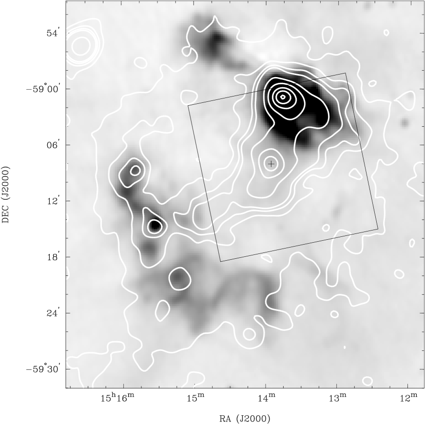
Figure 1.— A radio/X-ray comparison of G320.4–1.2. The greyscale corresponds to 843-MHz MOST observations (Whiteoak & Green (1996)), while the white contours represent smoothed ROSAT PSPC data (Trussoni et al. (1996)). Contour levels (in arbitrary units) are at levels of 0.5, 1, 1.5, 2, 5, 10, 20, 30 and 40. The position of PSR B1509–58 (as determined by G99) is marked by a “$+$” symbol. The central box delineates the Chandra ACIS-I field-of-view.

Figure 2.— Chandra image of G320.4–1.2 over the entire energy band. The image has been exposure-corrected and convolved with a gaussian of FWHM $10^{\prime\prime}$, and is displayed using a linear transfer function. The central black box in the main image shows the region covered by the panel at lower right. In this panel, the data have been smoothed with a gaussian of FWHM $4^{\prime\prime}$ and displayed using a logarithmic scale; the white box in this panel shows the region displayed in Figure 5. Specific features discussed in the text are indicated.

Figure 3.— A comparison of X-ray and radio emission in the region surrounding PSR B1509–58. The greyscale displays radio data from 1.4-GHz observations with the ATCA at a spatial resolution of $21^{\prime\prime}\times 24^{\prime\prime}$ and over a range 0 to 10 mJy beam^-1, as presented by G99. The ripples seen in the radio emission are residual sidelobes from the bright RCW 89 region to the north. The contours show Chandra data as in Figure 2, with contours at 0.5%, 2% and 30% of the peak.

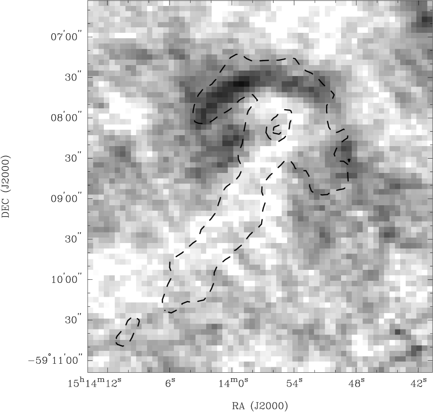
Figure 4.— Polarized radio emission in the region near the pulsar. The greyscale shows linearly polarized intensity at 5 GHz, at a spatial resolution of $6^{\prime\prime}\times 9^{\prime\prime}$ and over a range of 0 to 0.85 mJy beam^-1. The contours show Chandra data as in Figure 2, with contours at 2%, 20% and 50% of the peak.

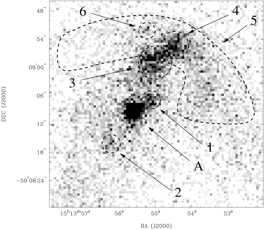
Figure 5.— X-ray emission immediately surrounding PSR B1509–58 in the energy range 0.3–8.0 keV. These data have been exposure-corrected but have had no smoothing applied. Specific features discussed in the text are marked and labeled.

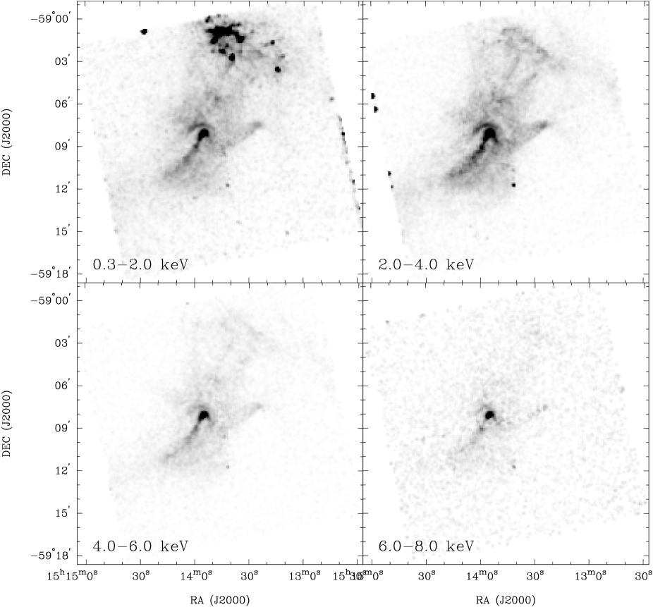
Figure 6.— As in Figure 2, but for four energy sub-bands.

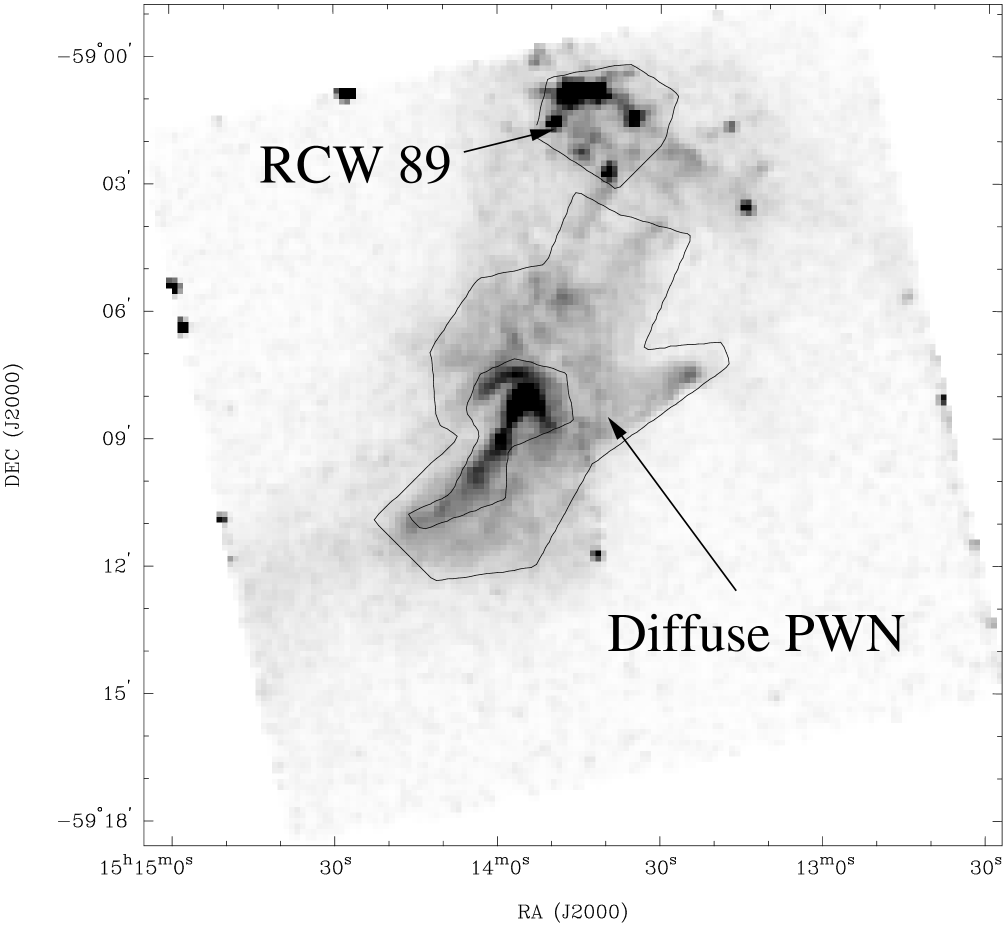
Figure 7.— A low-resolution version of Figure 2, showing the extraction regions used to generate the spectra shown in Figures 8 and 9. The region marked “Diffuse PWN” is an annular region which excludes regions A, C and E and features 1–5.

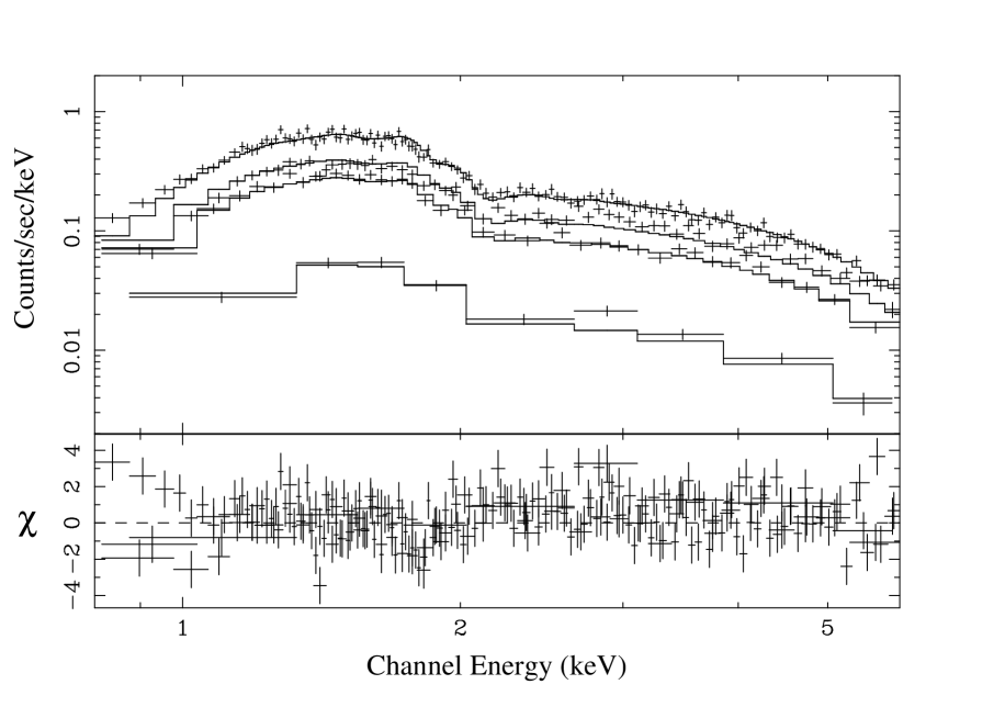
Figure 8.— X-ray spectrum of the diffuse pulsar wind nebula. The data-points in the upper panel show the data from each of the four CCDs on which the nebular emission falls, while the solid lines correspond to the best-fit absorbed power-law model. The lower panel shows the number of standard deviations by which the model and the data differ in each bin. The data have been plotted so as to give a signal-to-noise ratio of 10 in each bin.

Figure 9.— As in Figure 8, but for a spectral fit to the brightest clumps in RCW 89. In this case, the solid line corresponds to a non-equilibrium ionization model with variable abundances, and the data have been plotted with a signal-to-noise of 8 in each bin.

References

- Arendt (1991) Arendt, R. G. 1991, AJ, 101, 2160.
- Arons (1998) Arons, J. 1998, in Neutron Stars and Pulsars: Thirty Years after the Discovery, ed. N. Shibazaki, N. Kawai, S. Shibata, & T. Kifune, (Tokyo: Universal Academy Press), 339.
- Arons & Tavani (1993) Arons, J. & Tavani, M. 1993, ApJ, 403, 249.
- Aschenbach & Brinkmann (1975) Aschenbach, B. & Brinkmann, W. 1975, A&A, 41, 147.
- Bałucińska-Church & McCammon (1992) Bałucińska-Church, M. & McCammon, D. 1992, ApJ, 400, 699.
- Barnard & Arons (1982) Barnard, J. J. & Arons, J. 1982, ApJ, 254, 713.
- Bautz et al. (1998) Bautz, M. W. et al. 1998, Proc. SPIE, 3444, 210.
- Berghöfer, Schmitt, & Cassinelli (1996) Berghöfer, T. W., Schmitt, J. H. M. M., & Cassinelli, J. P. 1996, A&AS, 118, 481.
- Bhattacharya (1990) Bhattacharya, D. 1990, J. Astrophys. Astr., 11, 125.
- Bietenholz, Frail, & Hester (2001) Bietenholz, M. F., Frail, D. A., & Hester, J. J. 2001, ApJ, 560, 254.
- Blandford & Romani (1988) Blandford, R. D. & Romani, R. W. 1988, MNRAS, 234, 57P.
- Blondin, Chevalier, & Frierson (2001) Blondin, J. M., Chevalier, R. A., & Frierson, D. M. 2001, ApJ, 563, 806.
- Brazier & Becker (1997) Brazier, K. T. S. & Becker, W. 1997, MNRAS, 284, 335.
- Burke et al. (1997) Burke, B. E., Gregory, J., Bautz, M. W., Prigozhin, G. Y., Kissel, S. E., Kosicki, B. N., Loomis, A. H., & Young, D. J. 1997, IEEE Transac. Elec. Devices, 44, 1633.
- Caswell (1979) Caswell, J. L. 1979, MNRAS, 187, 431.
- Chagelishvili, Bodo, & Trussoni (1996) Chagelishvili, G. D., Bodo, G., & Trussoni, E. 1996, A&A, 306, 329.
- Chevalier (1998) Chevalier, R. A. 1998, Mem. Soc. Astron. It., 69, 977.
- Chevalier (2000) Chevalier, R. A. 2000, ApJ, 439, L45.
- Coroniti (1990) Coroniti, F. V. 1990, ApJ, 349, 538.
- Crawford, Manchester, & Kaspi (2001) Crawford, F., Manchester, R. N., & Kaspi, V. M. 2001, AJ, 122, 2001.
- du Plessis et al. (1995) du Plessis, I., de Jager, O. C., Buchner, S., Nel, H. I., North, A. R., Raubenheimer, B. C., & van der Walt, D. J. 1995, ApJ, 453, 746.
- Dubner et al. (2002) Dubner, G. M., Gaensler, B. M., Giacani, E. B., Goss, W. M., & Green, A. J. 2002, AJ, in press (astro-ph/0110218).
- Emmering & Chevalier (1987) Emmering, R. T. & Chevalier, R. A. 1987, ApJ, 321, 334.
- Frail et al. (1997) Frail, D. A., Bietenholz, M. F., Markwardt, C. B., & Ögelman, H. 1997, ApJ, 475, 224.
- Frail et al. (1996) Frail, D. A., Giacani, E. B., Goss, W. M., & Dubner, G. 1996, ApJ, 464, L165.
- Gaensler (2001) Gaensler, B. M. 2001, in Young Supernova Remnants (AIP Conference Proceedings Volume 565), ed. S. S. Holt & U. Hwang, (New York: AIP), p. 295.
- Gaensler et al. (1999) Gaensler, B. M., Brazier, K. T. S., Manchester, R. N., Johnston, S., & Green, A. J. 1999, MNRAS, 305, 724 (G99).
- Gaensler, Pivovaroff, & Garmire (2001) Gaensler, B. M., Pivovaroff, M. J., & Garmire, G. P. 2001, ApJ, 556, L107.
- Gallant & Arons (1994) Gallant, Y. A. & Arons, J. 1994, ApJ, 435, 230 (GA94).
- Gallant et al. (1992) Gallant, Y. A., Hoshino, M., Langdon, A. B., Arons, J., & Max, C. E. 1992, ApJ, 391, 73.
- Gotthelf & Wang (2000) Gotthelf, E. V. & Wang, Q. D. 2000, ApJ, 532, L117.
- Graham et al. (1996) Graham, J. R., Sankrit, R., Hester, J. J., Scowen, P. A., Michel, F. C., Watson, A., & Gallagher, J. S. 1996, BAAS, 188, 75.03.
- Greiveldinger et al. (1995) Greiveldinger, C., Caucino, S., Massaglia, S., Ögelman, H., & Trussoni, E. 1995, ApJ, 454, 855.
- Gvaramadze (2001) Gvaramadze, V. V. 2001, A&A, 374, 259.
- Helfand, Gotthelf, & Halpern (2001) Helfand, D. J., Gotthelf, E. V., & Halpern, J. P. 2001, ApJ, 556, 380.
- Hester (1998) Hester, J. J. 1998, Mem. Soc. Astron. It., 69, 883.
- Hester et al. (1995) Hester, J. J. et al. 1995, ApJ, 448, 240.
- Hester et al. (1996) Hester, J. J., Scowen, P. A., Sankrit, R., Michel, F. C., Graham, J. R., Watson, A., & Gallagher, J. S. 1996, BAAS, 188, 75.02.
- Hibschman & Arons (2001) Hibschman, J. A. & Arons, J. 2001, ApJ, 560, 871.
- Hjellming (1999) Hjellming, R. M. 1999, in Allen’s Astrophysical Quantities, 4th Edition, ed. A. N. Cox, (New York: Springer), 137.
- Hjellming & Johnston (1988) Hjellming, R. M. & Johnston, K. J. 1988, ApJ, 328, 600.
- Hoshino et al. (1992) Hoshino, M., Arons, J., Gallant, Y. A., & Langdon, A. B. 1992, ApJ, 390, 454.
- Kaaret et al. (2001) Kaaret, P. et al. 2001, ApJ, 546, 1159.
- Kardashev (1962) Kardashev, N. S. 1962, Sov. Astron., 6, 317.
- Kaspi et al. (2001) Kaspi, V. M., Gotthelf, E. V., Gaensler, B. M., & Lyutikov, M. 2001, ApJ, 562, L163.
- Kaspi et al. (1994) Kaspi, V. M., Manchester, R. N., Siegman, B., Johnston, S., & Lyne, A. G. 1994, ApJ, 422, L83.
- Kawai, Okayasu, & Sekimoto (1993) Kawai, N., Okayasu, R., & Sekimoto, Y. 1993, in Compton Gamma-Ray Observatory Symposium, ed. M. Friedlander, N. Gehrels, & D. J. Macomb, (New York: AIP), 213.
- (48) Kennel, C. F. & Coroniti, F. V. 1984a, ApJ, 283, 694.
- (49) Kennel, C. F. & Coroniti, F. V. 1984b, ApJ, 283, 710.
- Kuiper et al. (1999) Kuiper, L., Hermsen, W., Krijger, J. M., Bennett, K., Carramiñana, A., Schönfelder, V., Bailes, M., & Manchester, R. N. 1999, A&A, 351, 119.
- Lampland (1921) Lampland, C. O. 1921, Publ. Astr. Soc. Pacific, 33, 79.
- Lou (1998) Lou, Y.-Q. 1998, MNRAS, 294, 443.
- Manchester (1987) Manchester, R. N. 1987, A&A, 171, 205.
- Manchester & Durdin (1983) Manchester, R. N. & Durdin, J. M. 1983, in Supernova Remnants and Their X-Ray Emission (IAU Symposium 101), ed. J. Danziger & P. Gorenstein, (Dordrecht: Reidel), p. 421.
- Manchester, Tuohy, & D’Amico (1982) Manchester, R. N., Tuohy, I. R., & D’Amico, N. 1982, ApJ, 262, L31.
- Marsden et al. (1997) Marsden, D. et al. 1997, ApJ, 491, L39.
- Melatos (1998) Melatos, A. 1998, Mem. Soc. Astron. It., 69, 1009.
- Michel (1994) Michel, F. C. 1994, ApJ, 431, 397.
- Michel et al. (1996) Michel, F. C., Scowen, P. A., Hester, J. J., Graham, J., Watson, A., & Gallagher, J. 1996, BAAS, 188, 75.06.
- Milne, Caswell, & Haynes (1993) Milne, D. K., Caswell, J. L., & Haynes, R. F. 1993, MNRAS, 264, 853.
- Mineo et al. (2001) Mineo, T., Cusumano, G., Maccarone, M. C., Massaglia, S., Massaro, E., & Trussoni, E. 2001, A&A, 380, 695.
- Mori et al. (2002) Mori, K., Hester, J. J., Burrows, D. N., Pavlov, G. G., & Tsunemi, H. 2002, in Neutron Stars in Supernova Remnants, ed. P. O. Slane & B. M. Gaensler, ASP Conference Series, (San Francisco: Astronomical Society of the Pacific), in press (astro-ph/0112250).
- Muzzio (1979) Muzzio, J. C. 1979, AJ, 84, 639.
- Olbert et al. (2001) Olbert, C. M., Clearfield, C. R., Williams, N. K., Keohane, J. W., & Frail, D. A. 2001, ApJ, 554, L205.
- Orsatti & Muzzio (1980) Orsatti, A. M. & Muzzio, J. C. 1980, AJ, 85, 265.
- Pacholczyk (1970) Pacholczyk, A. G. 1970, Radio Astrophysics, (San Francisco: Freeman).
- Pacini & Salvati (1973) Pacini, F. & Salvati, M. 1973, ApJ, 186, 249.
- Pavlov et al. (2001) Pavlov, G. G., Kargaltsev, O. Y., Sanwal, D., & Garmire, G. P. 2001, ApJ, 554, L189.
- Pavlov et al. (2000) Pavlov, G. G., Sanwal, D., Garmire, G. P., Zavlin, V. E., Burwitz, V., & Dodson, R. G. 2000, BAAS, 196, 37.04.
- Pavlov & Zavlin (2000) Pavlov, G. G. & Zavlin, V. E. 2000, in Pulsar Astronomy — 2000 and Beyond, IAU Colloquium 177, ed. M. Kramer, N. Wex, & R. Wielebinski, (San Francisco: Astronomical Society of the Pacific), p. 613.
- Pelling et al. (1987) Pelling, R. M., Paciesas, W. S., Peterson, L. E., Makishima, K., Oda, M., Ogawara, Y., & Miyamoto, S. 1987, ApJ, 319, 416.
- Radhakrishnan & Deshpande (2001) Radhakrishnan, V. & Deshpande, A. A. 2001, A&A, 379, 551.
- Raymond & Smith (1977) Raymond, J. C. & Smith, B. W. 1977, ApJS, 35, 419.
- Rees & Gunn (1974) Rees, M. J. & Gunn, J. E. 1974, MNRAS, 167, 1.
- Romani & Yadigaroglu (1995) Romani, R. W. & Yadigaroglu, I.-A. 1995, ApJ, 438, 314.
- Sako et al. (2000) Sako, T. et al. 2000, ApJ, 537, 422.
- Sault, Bock, & Duncan (1999) Sault, R. J., Bock, D. C.-J., & Duncan, A. R. 1999, A&AS, 139, 387.
- Scargle (1969) Scargle, J. D. 1969, ApJ, 156, 401.
- Seward & Harnden Jr. (1982) Seward, F. D. & Harnden Jr., F. R. 1982, ApJ, 256, L45.
- Seward et al. (1983) Seward, F. D., Harnden Jr., F. R., Murdin, P., & Clark, D. H. 1983, ApJ, 267, 698.
- Seward et al. (1984) Seward, F. D., Harnden Jr., F. R., Szymkowiak, A., & Swank, J. 1984, ApJ, 281, 650.
- Spitkovsky & Arons (2000) Spitkovsky, A. & Arons, J. 2000, in Pulsar Astronomy — 2000 and Beyond, IAU Colloquium 177, ed. M. Kramer, N. Wex, & R. Wielebinski, (San Francisco: Astronomical Society of the Pacific), p. 507.
- Sulkanen & Lovelace (1990) Sulkanen, M. E. & Lovelace, R. V. E. 1990, ApJ, 350, 732.
- Tamura et al. (1996) Tamura, K., Kawai, N., Yoshida, A., & Brinkmann, W. 1996, PASJ, 48, L33.
- Tanvir, Thomson, & Tsikarishvili (1997) Tanvir, N. R., Thomson, R. C., & Tsikarishvili, E. G. 1997, New Astronomy, 1, 311.
- Tavani & Arons (1997) Tavani, M. & Arons, J. 1997, ApJ, 477, 439.
- Trussoni et al. (1996) Trussoni, E., Massaglia, S., Caucino, S., Brinkmann, W., & Aschenbach, B. 1996, A&A, 306, 581.
- Ulmer et al. (1993) Ulmer, M. P. et al. 1993, ApJ, 417, 738.
- van der Swaluw et al. (2001) van der Swaluw, E., Achterberg, A., Gallant, Y. A., & Tóth, G. 2001, A&A, 380, 309.
- (90) Weisskopf, M. C. et al. 2000a, ApJ, 536, L81.
- (91) Weisskopf, M. C., Tananbaum, H. D., Van Speybroeck, L. P., & O’Dell, S. L. 2000b, Proc. SPIE, 4012, 2.
- Whiteoak & Green (1996) Whiteoak, J. B. Z. & Green, A. J. 1996, A&AS, 118, 329. (http://www.physics.usyd.edu.au/astrop/wg96cat/).
- Willingale et al. (2001) Willingale, R., Aschenbach, B., Griffiths, R. G., Sembay, S., Warwick, R. S., Becker, W., Abbey, A. F., & Bonnet-Bidaud, J.-M. 2001, A&A, 365, L212.