LAL 01-71
October 2001

Laboratoire de l’Accélérateur Linéaire
CNRS-IN2P3 et Université Paris-Sud, Bât. 200, BP 34 - 91898 Orsay cedex

1 Introduction

EROS has discovered $\sim 70$ SNs during 8 periods partially dedicated to a SN search. The average discovery rate is 1 SN per 2 hours of observation, corresponding to expectation. Before 1999, the SNs that we discovered were publicly available on the web and reported in IAU telegrams. The low scientific return of this procedure convinced the EROS collaboration to work within a larger collaboration. Nevertheless, EROS has taken advantage of the homogeneity of its SNIa sample to obtain a SNIa explosion rate at $z\sim 0.1$[1].

EROS has participated in the large campaign of February-March 1999 lead by the SCP, which aimed at measuring $\sim 10$ SNIa’s discovered before or at maximum, including photometric and spectroscopic follow-up. EROS contributed an homogeneous sample of 8 SNIa’s discovered before maximum (of which 7 were monitored). Our procedure was as follows: The first SN detection was made on the day following the night during which 20 pictures (one square degree each) were taken. A confirmation picture was taken the following night, and the SN coordinates were then given to the coordinator. The complete process used to take less than 48 hours to provide a confirmed SN. This delay was clearly acceptable, if one considers the $\gtrsim 50\%$ proportion of pre-maximum SNIa’s delivered by EROS. A preliminary analysis of the photometric data collected for these SNIa’s is described in detail in Nicolas Regnault’s thesis[2].

The EROS-2 microlensing search will end at the end of 2002. In this document, we investigate a new way of using the EROS telescope (the MARLY) after this date.

2 The MARLY as a SN-photometer

2.1 Today’s status

The MARLY present optics has a wide aperture, and the sampling is relatively poor (EROS was designed to maximise the number of monitored stars per pixel). The pixel size is 0.6 arcsec. A test, done with the heat sources of the dome switched off, showed that the dome contribution to the experimental seeing was 0.8 arcsec on the optical axis. As there is a significant degradation of the seeing off-axis and because of the effect of the heat sources, the median instrumental seeing is only 1.5 arcsec.

2.2 Telescope configuration changes

The Marly telescope had originally a F/8 aperture. For the EROS programme, a focal reducer has increased the aperture to F/5. With the original aperture, a simple setup with a one-CCD camera and a BVRI filter wheel could be installed on the telescope.
We will also propose a more sophisticated setup to perform U band photometry in parallel with the other bands.

2.3 Optical photometer performances

In this section, we estimate the total time needed to fully monitor a SNIa with the MARLY telescope every other night in BVRI during 80 days after its discovery.

2.3.1 Expression of the exposure time

For a given passband $w$, the exposure time $T_{exp}$ needed to reach a relative photometric precision $\delta$ on a pointlike object with apparent magnitude $M_{w}$ depends on

• the photoelectron flux $\Phi_{w}(M_{w}=0)$ (in $\gamma e^{-}/s/m^{2}$) associated with a source of magnitude $M_{w}=0$, taking into account the detector efficiency,

• the magnitude of the background surface brightness $\mu_{w}$ per $arcsec^{2}$,

• the seeing.

For the MARLY collecting surface, the calculation and the validity conditions of the following formula are given in annex A:

$$\begin{split}T_{exp}&\simeq\frac{(175s)}{\left[\delta(in\%)\right]^{2}}\left[\frac{\Phi_{w}(M_{w}=0)}{10^{9}}\right]^{-1}\times\\ &\quad\times 10^{\frac{M_{w}-17.5}{2.5}}\left[0.27+1.59\sqrt{0.22+\left[\frac{seeing}{1\ arcsec}\right]^{2}10^{\frac{M_{w}-\mu_{w}}{2.5}}}\right]^{2}\end{split}$$ (1)

We will use this expression to perform a realistic simulation, taking into account real distributions for each parameter.

2.3.2 Photoelectron signal expected from the SNIa’s

By definition, $\Phi_{w}(M_{w}=0)$ depends on the spectrum of the measured point-like object. For SNIa’s, we estimate the number of photoelectrons produced in the detector in each of the UBVRI passbands by using the following ingredients:

• The photon spectra and the magnitudes of two typical SNIa’s:
  SN1990N, 7 days before and 7 days after maximum[3], and SN1994D, 3 days after maximum[4].

• The atmospheric transmission curve taken at airmass=1.

• The Bessel UBVRI theoretical transmission curves.

• The LBNL red-enhanced CCD spectral response.

• The transmission of the MARLY F/8 optics, which has been assumed to be uniform in wavelength, equal to 0.87 per reflector, i.e. $0.87^{2}=0.76$.

Fig. 1 shows the various transmission curves and the SN1994D spectrum.

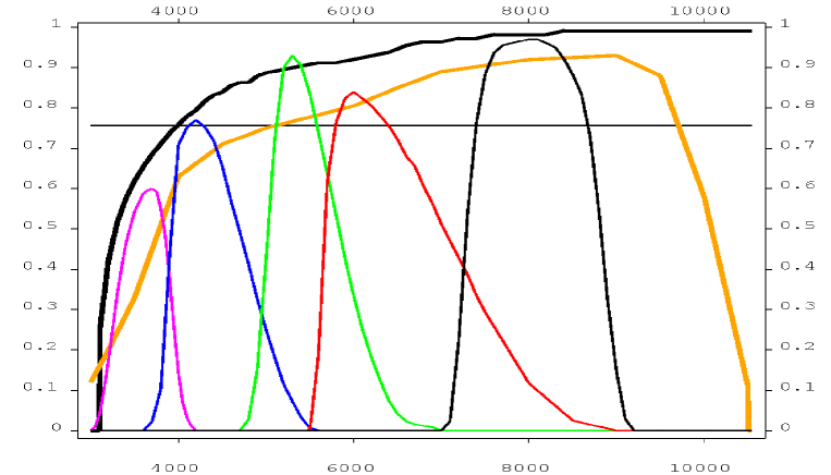
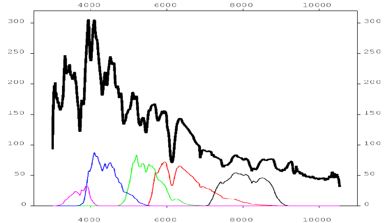
Figure 1: Upper panel: transmission of the UBVRI filters (coloured lines), the atmosphere (black thick), the optics (black standard), and quantum efficiency of the CCD (orange thick) as a function of the wavelength.
Lower panel: measured SN1994D spectrum in $photons/m^{2}/s/$Å, 3 days after maximum (black thick line), residual spectras after atmospheric, instrumental and filter transmissions, and conversion in the CCD in $\gamma e^{-}/m^{2}/s/$Å (coloured lines).

From this input, we find that a SNIa with $M_{\bf B}\simeq M_{\bf V}=0$, and a spectrum typical of the one emitted within +/-7 days from maximum, should produce a flux of photoelectrons in the detector given by the upper part of Table 1.

Table 1: The expected total $\gamma e^{-}$ fluxes produced by the LBNL red-enhanced CCD at Airmass=1 for a SNIa at maximum in B. The collecting area of the MARLY is $S=0.57\ m^{2}$.

$\Phi_{w}({\bf B}=0)=$Flux ($\gamma e^{-}/m^{2}/s$) for SNIa with $M_{B}=0$
Filter w		U	B	V	R	I
Magnitude		-0.58	0.	0.09	0.03	0.29
$\Phi_{w}({\bf B}=0)\ (10^{9}\ \gamma e^{-}/m^{2}/s)$		$0.9$	$4.$	$3.9$	$5.2$	$3.7$
$\Phi_{w}(M_{w}=0)=$Flux ($\gamma e^{-}/m^{2}/s$) for SNIa with $M_{w}=0$
Magnitude		0.	0.	0.	0.	0.
$\Phi_{w}(M_{w}=0)\ (10^{9}\ \gamma e^{-}/m^{2}/s)$		$0.54$	$4.$	$4.2$	$5.3$	$4.8$
Expected total flux for the MARLY ($\gamma e^{-}/s$)
$F^{SN}_{w}=S\times\Phi_{w}(B=0)\times 10^{-M_{B}/2.5}$
redshift	at max	U	B	V	R	I
0.01	Magnitude	13.3	13.9	14.0	13.9	14.2
	$F^{SN}$	1440	6280	6120	8160	5810
0.05	Magnitude	16.8	17.4	17.5	17.4	17.7
	$F^{SN}$	58	250	244	325	231
0.1	Magnitude	18.3	18.9	19.0	18.9	19.2
	$F^{SN}$	14	63	61	82	58

Taking into account the measured colour indices of SN1994D, we get a correspondance between the zero $M_{w}$ magnitudes and the photoelectron fluxes in UBVRI (lower part of Table 1) .

2.4 SN photometry simulation

We have computed the total time spent in the photometric follow-up using a simple SN light curve simulation. We suppose all SNe to lie at $z=0.05$. The whole calculation is done for airmass=1. The SN discovery age is supposed to range between 5 and 10 days before the time of B maximum with a flat distribution. The lunar phase is also randomly chosen.

2.4.1 SN environnement - Expected photoelectron background

The background surface magnitude due to both the sky brightness and the host galaxy surface brightness in the w passband is given by:

$$\mu_{w}=-2.5log_{10}\left(10^{-\mu_{w}^{gal}/2.5}+10^{-\mu_{w}^{sky}/2.5}\right)$$

When the background flux is negligible (i.e. $\mu_{w}$ is large, or if the SN is bright), the last factor in the expression of $T_{exp}$ is 1, and the formula can be simplified.

• Night sky brightness $\mu_{w}^{sky}$
  The sky brightness depends on the Moon phase and also on the atmospheric conditions. We adopt the average values used for the preparation of the ESO proposals (Table 2, upper part).

  Table 2: Sky brightness in magnitudes for different passbands, as a function of the number of days from the New Moon; range and average of the host galaxy brightness. All magnitudes are the ones at the top of the atmosphere.
  

  Days from	Sky brightness
  New Moon	U	B	V	R	I
  0	22.0	22.7	21.8	20.9	19.9
  3	21.5	22.4	21.7	20.8	19.9
  7	19.9	21.6	21.4	20.6	19.7
  10	18.5	20.7	20.7	20.3	19.5
  14	17.0	19.5	20.0	19.9	19.2
  host galaxy brightness
  min.	22.	22.	21.5	21.	20.5
  average	21.	21.	20.5	20.	19.5
  max.	19.	19.	18.5	18.	17.5

• Host galaxy brightness $\mu_{w}^{gal}$
  The background light from the host galaxy depends on the position of the SN. If the SN is in the disk, far from the bulge, then the average surface brightness of the galaxy in B is $\mu^{gal}_{\bf B}=22.4$ [5]. If the SN is located in the bulge, the average is $\mu^{gal}_{\bf B}\sim 20$. The SNIa’s referred to in the EROS paper[1] have a local host surface brightness ranging between $\mu^{gal}_{\bf B}=19$ and $\mu^{gal}_{\bf B}=22$, and more than 80% have $\mu^{gal}_{\bf B}>20$ (see Fig. 2). Following [5] we adopt $<\mu^{gal}_{\bf U}-\mu^{gal}_{\bf B}>\sim 0$ and $<\mu^{gal}_{\bf B}-\mu^{gal}_{\bf R}>\sim 1$ as typical values, and we extrapolate for V and I.

  

  Figure 2: Distribution of the host galaxy B-magnitude in the EROS SNIa discovery sample.

  In the following, we will assume that the SNIa’s that we will follow-up will belong to such a sample.

2.4.2 SN light curve simulation

Light curves of SNIa’s at $z=0.05$ are generated according to the observed frequency of various templates described in [2].

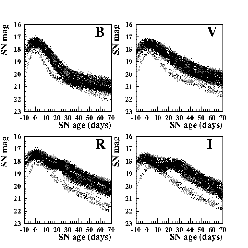
Figure 3: SN Light curves (in mag) obtained in the simulation.

SNIa light curves show some diversity. We use B,V,R and I templates obtained in [2] to describe the different luminosity evolutions with time. We used those templates from reference [2] for which early data is available . The absolute peak magnitude attributed to each template is based on the standardisation relation determined in [2].

The program randomly generates a template according to the frequency distribution which came out of in the best fit analysis of [2]. The SN maximal luminosity is smeared using a normal law with 0.1 mag dispersion (in each band). For each SN, a host surface brightness is generated according to the distribution shown in Fig. 2. Once a discovery age, lunar phase, host brightness and SN subtype have been determined, the program follows the SN luminosity evolution for 70 days after B maximum. Photometric measurements are assumed to take place every other night, and a 70% good weather is assumed. In a bad weather case, the new measurement is attempted again the next day. 1000 light curves obtained this way are shown in figure 3. We associate a random seeing to each measurement, using the true seeing distribution of La Silla (see Fig. 4); an instrumental contribution of $0.8^{\prime\prime}$, as measured on the MARLY optical axis, is quadratically added to this seeing.

Figure 4: Distribution of the seeing at La Silla (in arcsec).

The exposure time necessary to reach a 2% photometric precision is then computed for each measurement. These times are shown in figure 5. These exposure calculations are done for the MARLY telescope. The scaling to be performed in order to get results for another telescope (at the same site) or another resolution is straightforward.

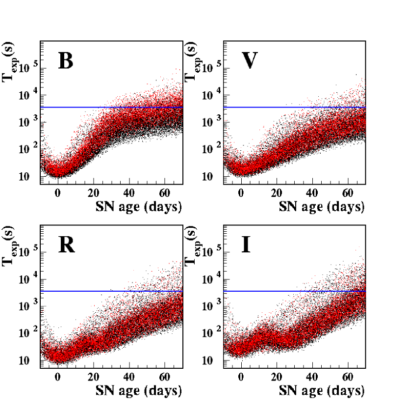
Figure 5: $Log_{10}(T_{exp})$ needed to reach 2% photometric precision versus the SN age (in days). Exposures taken around full moon ($\pm 4$ days) are shown in red. The horizontal lines illustrates the 1 hour cutoff used in this study.

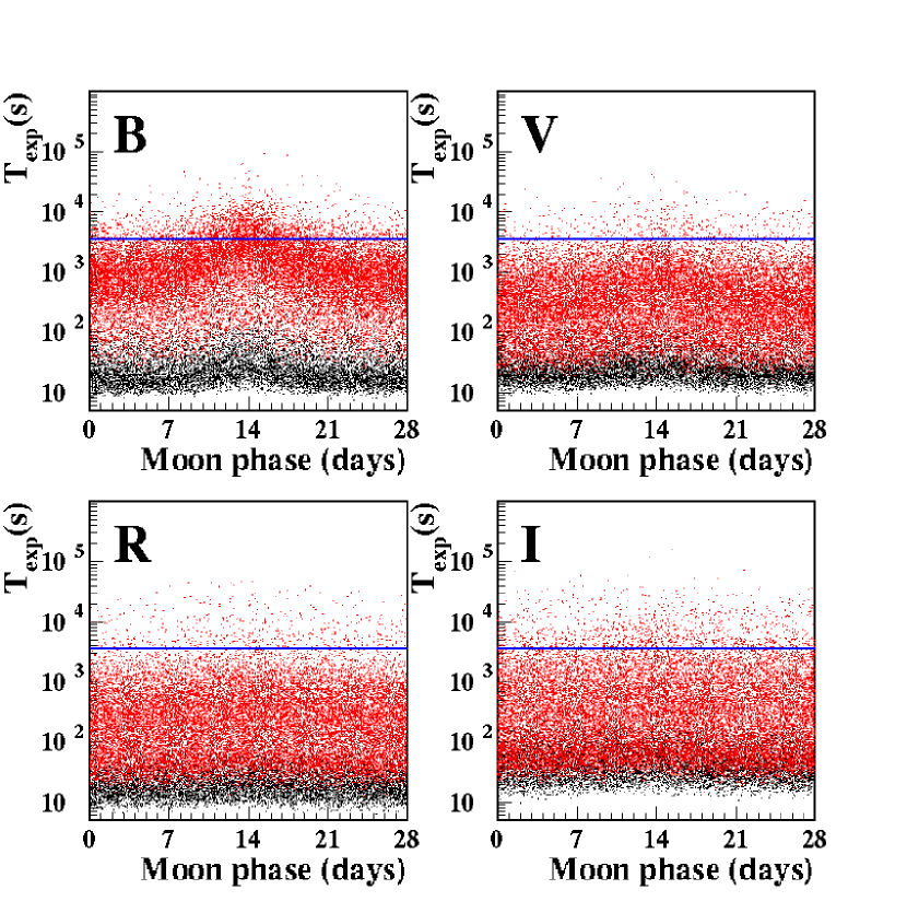
Figure 6: $Log_{10}(T_{exp})$ needed to reach 2% photometric precision versus the Moon phase (in days). The red dots correspond to $SN\ age>15\ days$. For these late measurements, the exposure times are much longer and strongly depend on the Moon phase. The horizontal lines illustrates the 1 hour cutoff used in this study.

Figure 7: Distribution of the total follow-up time per simulated SNIa, in hours. Each entry corresponds to the sum of the exposure times of about 40 measurements with 2% photometric precision.

2.5 The “cost” of a SNIa

Fig. 5 and 6 give the distribution of exposure times as a function of SN age and Moon phase respectively. Long exposure times occur when the SNIa fades, typically from 15 days after maximum (red dots in Fig. 6). The exposure then strongly depends on the sky brightness in B and V.

We estimate the telescope time needed per SNIa by adding the exposure times of all the measurements (about 40 measurements per SNIa and per passband). An overhead of 60 s is added to each exposure. For long exposures, which will be fractionned, we further add 60 s of overhead to every sequence of 20 minutes of observation. We choose to truncate the exposures at 3600 seconds. Such a truncation affects 7% of the measurements and takes place only in the late part of the SN light curves ($age>30\ days$). The photometric resolution is then slightly downgraded (from 2% to 4% in the worst case). Fig. 7 shows the histogram of the total telescope time for each passband, for our sample of 1000 simulated SNIa’s. The outcome of this study is that the follow-up of a SNIa, involving about 40 measurements regularly spaced within a 80 day period, needs an average telescope time of:

• 9.5 hours in B,

• 4.5 hours in V,

• 3.8 hours in R,

• and 5.3 hours in I,

Table 3 gives the results of the same calculations done for other CCD efficiencies (see Fig. 8).

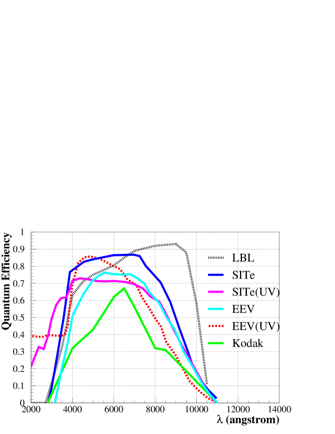
Figure 8: CCD efficiencies used in the calculation.

Table 3: Total follow-up time (hours) for 4 CCD efficiencies, in the BVRI bands

. CCD B V R I Total Berkeley 9.5h 4.5h 3.8h 5.3h 23.1 SITe 8.6h 4.2h 3.7h 6.2h 22.7 EEV 10.6h 4.6h 4.2h 7.0h 26.4 Kodak 14.1h 6.1h 4.9h 9.4h 34.5

2.6 Strategy

In order to minimize the cost of the measurements taken during the late section of a SNIa (when faintest) we could consider some improvement to the very simple strategy described above:

• As long as the SNIa (at $z=0.05$) is close to its maximum ($\sim 17.5$), one can neglect the sky brightness in BVRI and the host galaxy luminosity in a first approximation. This is no longer the case when the SN fades. Then, when the Moon is bright, we should favour data taking on the brightest SNIa’s, and devote the dark fraction of each night to the observation of the faintest ones.

• As the luminosity variations of “old” SNIa’s are slow, relaxing the sampling rate should have less impact than around the maximum.

• Lastly, we could downgrade the photometric precision when the estimated exposure time is long. The impact of such a choice should be studied.

2.7 An additional dedicated camera for U

The U band is of special interest, because the detailed study of the light curves of the nearby SNIa’s will be useful for the I band study of high redshift SNIa’s ($z>1$).

For this passband, only two SNIa templates are available. The first order calculation performed in the first version of this note (May 2001) showed that more than 60 hours were needed to follow-up a SNIa in U band, with our simple strategy. Figure 9 shows the individual exposures in U, computed as for the other filters for the Berkeley CCD, as a function of the SN age and lunar phase.

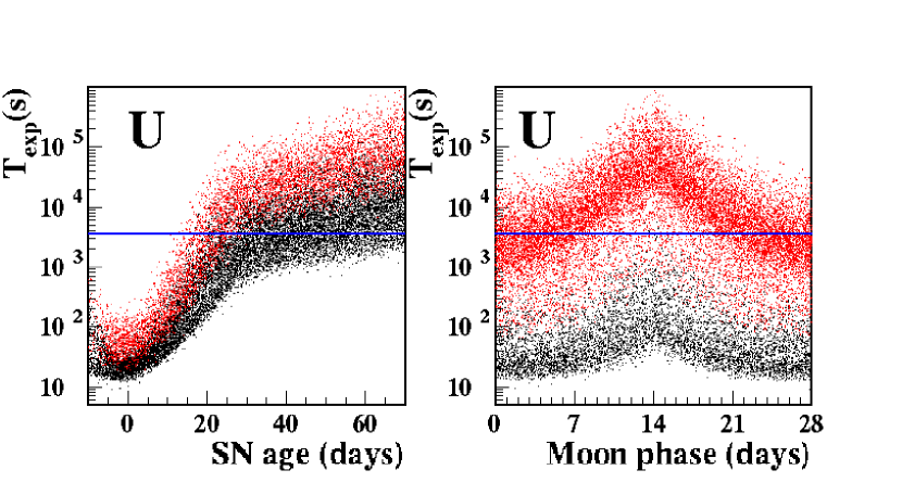
Figure 9: Exposures needed to reach a 2% photometric precision in U versus the SN age (left) and Moon phase (right) with the Berkeley CCD. The colors are drawn as for figures 5 and 6. The horizontal lines correspond to 1 hour.

Since unrealistically long exposures are needed for the U band, we have considered the possibility to take images in parallel in the U band and in BVRI with a dichroic beam splitter. A possible setup to achieve this is displayed on figure 10. Preliminary discussions with optics engineers from Observatoire de Marseille confirmed the technical feasibility of this setup.

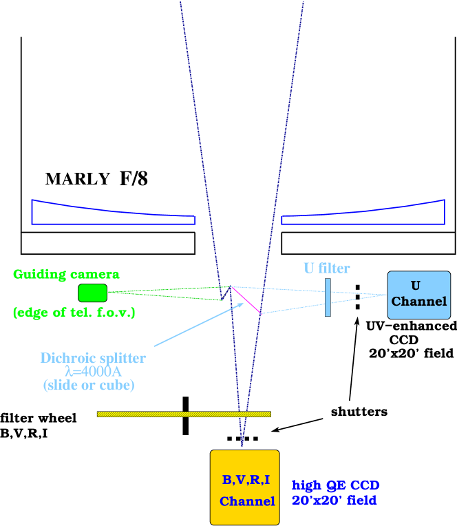
Figure 10: A possible setup for a photometer integrating in U and in BVRI in parallel

In this setup the CCD detectors can be separately optimized for the U and the BVRI bands. The data taking could proceed as follows. Consecutive exposures in BVRI are chosen so as to ensure a 2% photometric resolution. The exposure in U lasts until the end of this cycle. To evaluate the viability of this scheme, we have estimated the resulting photometric precision in U. We have assumed that the UV-enhanced SITe CCD will be used for this channel (see figure 8). Figure 11 shows these individual resolutions as a function of the SN age and lunar phase.

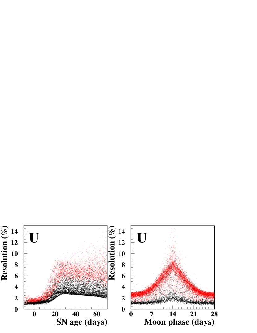
Figure 11: Photometric resolutions achieved when exposing in U with a SITe UV-enhanced device, in parallel with BVRI and the LBL CCD, as a function of SN age and Moon phase. Red points indicate measurements scheduled near full Moon (left) or at a SN older than 15 days (right).

Figure 12: Photometric resolutions achieved when exposing in U with a SITe UV-enhanced device in parallel with BVRI and the LBL CCD. This corresponds to a strategy aiming at a 2% resolution in BVRI.

The moon has clearly a strong degrading effect (near full moon) ; late epochs (after day 25) are also attributed a worse resolution.

Figure 12 shows the resolutions achieved with the naive strategy discussed here. Almost all measurements have a resolution better than $\approx 10\%$. The average resolution is $\approx 3.5\%$. A more subtle observing strategy could be sought to optimize the achieved resolutions versus the observing time. For example, one could decide to sometimes impose the BVRI exposures to reach a fixed, better resolution in U.

The numbers obtained here in the U passband are somewhat uncertain because of the large fluctuations of the atmospheric absorption. However, since exposures in U and other bands are simultaneous, color dependent absorption corrections due to variations in atmospheric conditions should be controlled. Monitoring these absorption corrections will be easier with a larger CCD field ; $2k\times 2k$ chips are at least necessary .

Finally, it is worth to mention that a factor of 2 in the photo-electron flux in U could be gained by removing the U filter. The effective passband (limited by the atmospheric absorption cutoff and the dichroic) would then be slightly modulated by the atmospheric conditions. This solution, still under study, might be considered only if the absorption is proved to be precisely monitored.

2.8 Maximum number of SNs that can be monitored

Data will be taken sequentially with the BVRI filters. The total telescope time per SNIa will thus be: 9.5+4.5+3.8+5.3=23.1 hours, spread over a period of 80 days. The average duration of the astronomical night at La Silla is 9 hours, and the average clear sky fraction is 70%. Then the average available time per period of 80 days is 80x9x0.7=504 hours. Up to 22 SNIa’s can be completely measured during this period of 80 days. Therefore the rate of 100 SNIa’s per year completely measured in the UBVRI passbands is the capacity of the MARLY with the setup outlined in figure 10. This rate could be made larger with a more subtle strategy as indicated above with a limited loss in sampling or in photometric precision. By using the tables and figures provided in this note, the reader can estimate the performance that would correspond to another strategy.

2.9 Miscellaneous

One should keep in mind that we have considered SNIa’s with no reddening in our calculations. In the case of reddening, the estimates in the blue passbands may be significantly affected.

For the U band, airmass is a critical issue since the atmospheric absorption is a dominant factor. The signal from the SN and the host galaxy would be lowered by a factor 1.22 if the airmass were 1.5 instead of 1, and it is clear that the full Moon would strongly disturb the observations in this passband.

Due to the presence of a dichroic splitter, the effective B band could be slightly narrower than the standard one.

From figure 1 one may see that this setup is also sensitive in the Z band which could be added to our observation scheme in addition with BVRI. Nearby SNIa have not yet been thoroughly studied in this band which could be helpful to disentangle the SN reddening by the host galaxy’s dust and the intrinsic SN colour dispersion. Finally, let us recall that the proposed configuration could be optimized to other photometric systems (e.g. $ugriz$).

2.10 Necessary upgrades and schedule

To use the MARLY as a photometer, according to our preliminary design, the following technical changes must be done:

• The focal reducer has to be removed, and the F/8 optics has to be re-installed. A dichroic beam splitter at a wavelength near 4000 Å should be installed. Moreover, the guiding system has to be adapted.

• two CCD cameras have to be built :

  • A single CCD camera with a high performance CCD for BVRI,

  • A single CCD camera with a UV-enhanced CCD for U.

The EROS project will stop taking data at the end of december 2002. Designing and building the instrument can be largely decoupled from MARLY running and thus could be performed in France. Installing and testing the system on site should not take longer than one month, as in the EROS2 case. Provided a more general framework is found for this project, a startup as early as spring 2003 could take place.

2.11 Expected performance

Around 100 SNIa’s per year at $z\sim 0.05$ could be fully followed-up in BVRI with a photometric precision $\delta=2\%$, and in the same time in U with a 3.5% photometric precision on average. The exposure time scales with $\delta^{-2}$. If the overhead time is small compared to the exposure time (if $\delta<2\%$), then the number of SNIa’s that can be monitored is $\sim 25\times\delta(\%)^{2}$ per year. If $\delta>2\%$, then the overhead time is not negligible and we have to use the following expression

$$T_{telescope}\sim 40\times(<T_{exp}>+T_{overhead})$$

to correctly estimate the corresponding telescope time and the rate of monitored SNIa’s. We thus find that around 300 SNIa’s per year at $z\sim 0.05$ could be fully followed-up with a $\delta=4\%$ photometric precision in BVRI.

3 Conclusion

Other possible uses (as a SN discoverer or with an integral field spectrometer) of the 1 meter dedicated MARLY telescope, based at La Silla, have also been evaluated in a more complete studiy available on request.

Refurbished in order to simultaneously perform BVRI and U photometry, the MARLY could be used for the complete follow-up (40 measurements spanning 80 days) of at least 100 SNIa’s per year at $z\sim 0.05$, with a photometric precision of 2% in BVRI and 3.5% on average in U. If the required photometric precision is only 4%, then about 300 SNIa’s can be followed-up each year.

A project dedicated to the nearby SN study should integrate dedicated discovery and follow-up means, the latter providing spectrographic and/or photometric capabilities. With the equipment proposed in this note, the MARLY telescope could nicely complement such a project. We will would be happy to collaborate on any such project.

Annex A
Expression of the optimal photometric precision accessible with aperture
photometry

Let

• $T_{exp}$ be the exposure time (in s),

• $F^{SN}$ be the integrated photoelectron flux from the SN in the telescope in photo-electrons per second ($\gamma e^{-}/s$),

• $b$ be the photoelectron flux per pixel originating in the atmospheric emission and the host galaxy (in $\gamma e^{-}/s$)

• $p$ be the pixel size.

Assuming that the PSF is a gaussian of standard deviation $\sigma=seeing/2.36$:

$$PSF(r)=\frac{F^{SN}\times T_{exp}}{2\pi\sigma^{2}}e^{-r^{2}/2\sigma^{2}},$$

and that the pixel size is small with respect to the seeing, the time integrated photoelectron signal in a disk of radius r is given by

$$S(r)=F^{SN}\times T_{exp}\times(1-e^{-r^{2}/2\sigma^{2}}).$$

During the same exposure time, the number of photoelectrons due to the atmosphere and the host galaxy in the disk of radius r is given by

$$B(r)=b\times T_{exp}\times\pi\left[\frac{r}{p}\right]^{2}.$$

Assuming that we measure separately $<B(r)>$ with a negligible uncertainty, then the fluctuation of the sum $S(r)+B(r)-<B(r)>$ is given by

$$\sigma(r)^{2}=S(r)+B(r)+\sigma_{e}^{2}\times\pi\left[\frac{r}{p}\right]^{2},$$

where $\sigma_{e}$ is the readout noise per pixel. The photometric resolution is then given by the ratio $\delta=\frac{\sigma(r)}{S(r)}$. The resolution $\delta$ has its smallest value when $\frac{d\delta}{dr}=0$. Expressing this condition leads to the calculation of the optimal value of r, and the expression of the best resolution follows:

$$\delta=[F^{SN}\times T_{exp}]^{-\frac{1}{2}}\times D,$$

where D is a “degradation” factor of the resolution, depending only on the noise to signal ratio in the pixel where the signal is maximal:

$$R=\frac{bT_{exp}+\sigma_{e}^{2}}{F^{SN}T_{exp}/2\pi\left[\frac{\sigma}{p}\right]^{2}}=\frac{total\ noise/pixel}{peak\ flux\ of\ the\ SN/pixel}.$$

For long exposures, the electronic readout noise will always be negligible compared to the fluctuations of the background brightness. Then R can be written:

$$R=1.13\left[\frac{seeing}{1\ arcsec}\right]^{2}10^{\frac{M-\mu}{2.5}},$$

where M is the magnitude of the SN and $\mu$ is the total background magnitude per $arcsec^{2}$. The D factor variation with R is given in Fig. 13 ;

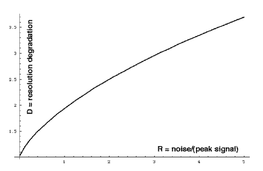
Figure 13: The degradation factor D of the resolution as a function of the ratio R of the noise per pixel to the maximum signal per pixel.

we easily check that for R=0 (no background), the resolution is simply given by the gaussian fluctuation of the number of signal photoelectrons, as expected. The following formula is an excellent approximation (within 2%) of D, at least up to R=10:

$$D\simeq 0.27+1.5\sqrt{R+0.25}.$$

For a given passband $w\in\{{\bf UBVRI}\}$, $F^{SN}_{w}$ is related to the $M_{w}$ magnitude of the SN and to the collecting surface S of the telescope through the relation:

$$F^{SN}_{w}=\Phi_{w}(M_{w}=0)\times S\times 10^{-M_{w}/2.5},$$

where $\Phi_{w}(M_{w}=0)$ is the photoelectron flux in the w passband per second per $m^{2}$ collecting surface, for a SNIa with magnitude $M_{w}=0$. Then the exposure time $T_{exp}$ needed to reach a photometric precision $\delta$ is given by the expression:

$$T_{exp} = \frac{D^{2}}{F^{SN}_{w}\times\delta^{2}}$$

$$= \frac{10^{M_{w}/2.5}}{S\times\Phi_{w}(M_{w}=0)}\times\frac{D^{2}}{\delta^{2}}$$

$$\simeq \frac{10^{M_{w}/2.5}}{S\Phi_{w}(M_{w}=0)}\frac{1}{\delta^{2}}\left[0.27+1.5\sqrt{0.25+1.13\left[\frac{seeing}{1\ arcsec}\right]^{2}10^{\frac{M_{w}-\mu_{w}}{2.5}}}\right]^{2}.$$

This exposure time scales with the inverse of the telescope collecting power (surface $\times$ transmission) and with the inverse of the square of the requested resolution. The scaling with the seeing is more complex, and depends on the contrast between the signal (from the SN) and the background flux.

For the MARLY telescope $S=\frac{\pi}{4}\times(d_{prim.}^{2}-d_{sec.}^{2})=0.57\ m^{2}$ where $d_{prim.}=0.98~{}m$ is the primary mirror diameter and $d_{sec.}=0.49~{}m$ is the diameter of the obstructing secondary mirror. Then $T_{exp}$ can be expressed as follows :

$$\begin{split}T_{exp}&\simeq\frac{(175s)}{\left[\delta(in\%)\right]^{2}}\left[\frac{\Phi_{w}(M_{w}=0)}{10^{9}}\right]^{-1}\times\\ &\quad\times 10^{\frac{M_{w}-17.5}{2.5}}\left[0.27+1.59\sqrt{0.22+\left[\frac{seeing}{1\ arcsec}\right]^{2}10^{\frac{M_{w}-\mu_{w}}{2.5}}}\right]^{2}.\end{split}$$

When the background flux is negligible (i.e. if $\mu_{w}$ is large, or if the SN is bright), the last factor in the expression of $T_{exp}$ is 1, and the formula can be simplified.

References

- [1] EROS coll. 2000, A&A 362, 419-425.
- [2] Regnault N. 2000, PhD thesis, LAL00-65 report.
- [3] Leibundgut B. et al. 1991, ApJ 371, L23-L26.
- [4] Meikle W.P.S. et al. 1996, MNRAS 281, 263-280.
- [5] Rolf A. Jansen et al. 2000, ApJ Suppl. Series 126, 271-329.