Probing the mass distribution in groups of galaxies using gravitational lensing

Abstract

In this paper, we study gravitational lensing by groups of galaxies. Since groups are abundant and therefore have a large covering fraction on the sky, lensing by groups is likely to be very important observationally. Besides, it has recently become clear that many lens models for strong lensing by individual galaxies require external shear to reproduce the observed image geometries; in many cases a nearby group is detected that could provide this shear. In this work, we study the expected lensing behavior of galaxy groups in both the weak and strong lensing regime. We examine the shear and magnification produced by a group and its dependence on the detailed mass distribution within the group. We find that the peak value of the weak lensing shear signal is of the order of 3 per cent and varies by a factor of about 2 for different mass distributions. These variations are large enough to be detectable in the Sloan Digital Sky Survey (SDSS). In the strong lensing regime we find that the image geometries and typical magnifications are sensitive to the group properties and that groups can easily provide enough external shear to produce quadruple images. We investigate the statistical properties of lensing galaxies that are near or part of a group and find that statistical lens properties, like the distribution of time delays, are affected measurably by the presence of the group which can therefore introduce an additional systematic error in the measurement of the Hubble constant from such systems. We conclude that both the detection of weak lensing by groups and accurate observations of strong galaxy lens systems near groups could provide important information on the total mass and matter distribution within galaxy groups.

1 Introduction

Gravitational lensing by isolated galaxies and clusters of galaxies has been used extensively both as a cosmological tool (Bartelmann et al. 1998; Wambsganss, Cen & Ostriker 1998) and as a method to map detailed mass distributions (Mellier 1999). In the weak lensing regime, reconstruction methods have provided moderate-resolution shear maps (Hoekstra et al. 1998; Clowe et al. 2000; Hoekstra, Franx & Kuijken 2000). In analyses that combine both weak and strong lensing data for clusters it is found that further constraints can be obtained on the clumpiness of the dark matter distributions on smaller scales within clusters (Natarajan & Kneib 1997; Geiger & Schneider 1999). This is done exploiting the fact that image multiplicities and geometry are well understood in the strong lensing regime for the HST cluster lenses, and combining with ground-based weak shear data, mass models for the critical regions of both clusters and the galaxies therein can be constructed (Natarajan et al. 1998).

Within the context of the current paradigm for structure formation – gravitational instability in a cold dark matter dominated Universe leading to mass hierarchies – clusters and isolated galaxies are at extreme ends of the mass spectrum of collapsed structures. Clusters are the most massive, virialized objects, have the highest density contrast and are rare, whereas galaxies are less massive and more abundant. In this scenario, groups of galaxies, which lie in the intermediate mass range between galaxy clusters and individual galaxies, are the most common gravitationally bound entities at the present epoch (Ramella, Pisani & Geller 1997). Galaxy groups contain between 3 and 30 galaxies and they trace the large-scale structure of the Universe (Ramella et al. 1999). The abundance of compact groups was estimated by Barton et al. (1996) to be quite high, $1.4\times 10^{-4}\,h^{-3}\,Mpc^{-3}$. It is likely that they contribute significantly to the mass density of the Universe, $\Omega_{\mathrm{M}}$. Probing the mass of groups and the mass distribution within groups is likely to be crucial to understanding the evolution of both dark and baryonic matter.

In this paper we present numerical investigations of both the weak and strong lensing signal expected from groups of galaxies. In § 2, a brief overview of galaxy groups is presented, concentrating on the properties of the observed compact Hickson groups (Hickson 1982), followed by a description of the properties of the simulated groups. In § 3 the lensing properties of the mass models is outlined along-with a brief description of the numerical analysis techniques. § 4 focuses on the expected weak lensing signal from groups of galaxies and its dependence on group properties. In § 5, the effects of a group in the vicinity of a strong galaxy lens are studied. The paper concludes with a summary of the results and suggestions for a possible strategy for the constraining the detailed mass distribution within galaxy groups in § 6.

2 Properties of Galaxy groups

The details of the distribution of dark matter in galaxy groups is poorly understood at present. It is not known if there exists a common dark matter potential well for the group as a whole or if the dark matter content of the group is simply dominated by the individual halos of the member galaxies. X-ray surface brightness profiles seem to point towards the existence of a common group halo for compact groups (Ponman et al. 1995; Helsdon et al. 2001), as extended and diffuse X-ray emission is detected from the group as a whole, although it is often observed to be centered around the optically brightest galaxy in the group (Mahdavi et al. 2000).

The precise morphology of the dark matter distribution in groups can provide important theoretical constraints on their formation and future evolution. Gravitational lensing offers an elegant method to map the mass content of the group and a first observational detection has been reported by (Hoekstra et al. 2001). For groups 50 selected from the Canadian Network for Observational Cosmology Galaxy Redshift Survey (CNOC2) at $z=0.12-0.55$, they report a typical mass-to light ratio in solar units in the B-band of 191$\pm$83 h, lower than what is found for clusters indicating the presence of dark matter in groups. Since the lensing effects of individual galaxies are detectable at a significant level (commonly referred to as galaxy-galaxy lensing, see Brainerd, Blandford & Smail 1996), we expect an unambiguous signal to be obtained for groups. The prospect of combining lensing data with X-ray data to probe the mass distribution in galaxy groups is promising, specially in the light of current high-resolution imaging X-ray satellites (Markevitch et al. 1999; Ettori & Fabian 2000).

Detected galaxy groups have been found in two primary configurations: compact and loose. The identification of groups and the establishment of membership has proven to be difficult due to the ambiguity arising from chance superpositions on the sky (Hickson et al. 1992; de Carvalho & Djorgovski 1995; Barton et al. 1996; Zabludoff & Mulchaey 1998, 2000). Targeted spectroscopic surveys for groups are needed in order to document and define the galaxies that constitute a group (Humason et al. 1956; Barton et al. 1996; Ramella et al. 1997). Studies of the morphological composition of compact groups (Williams & Rood 1987; Hickson et al. 1988) indicate that the fraction of late-type spiral galaxies in these environments is significantly lower than in the field. Additionally, there is evidence that the faint end of the luminosity function of compact groups is depleted and the bright end may be brightened (Barton et al. 1996). Even when redshifts are known for the group members, it is still sometimes unclear whether or not they constitute a gravitationally bound structure. From the velocity histogram of the members while it often appears that the groups are bound, they appear to be unvirialized (Zabludoff 2001). Extended X-ray emission detected from hot plasma that is confined in the gravitational well provides conclusive evidence for a group being gravitationally bound (Mahdavi et al. 2000; Helsdon & Ponman 2000).

Compact groups have been cataloged by (Hickson 1982) and are easily identified on the sky due to the high projected over-density of member galaxies, but might not be truly representative of groups as a whole. There has been some recent evidence from the studies of a large sample of loose groups (Helsdon & Ponman 2000) that the correlations observed between their properties, such as X-ray luminosity, velocity dispersion and temperature, differ from those of compact groups studied by Mulchaey & Zabludoff (1998). The mass function of nearby galaxy clusters follows a Press–Schechter form (Press & Schechter 1974), and recent studies have shown that the mass function of loose groups follows a similar distribution (Girardi & Giuricin 2000), suggesting a continuity of clustering properties from groups to rich clusters. However, the detailed mass distribution in galaxy groups has not been investigated so far. In particular, it is still unclear whether the majority of groups possess a massive group dark matter halo, as suggested by the observed X-ray emission of some groups. Gravitational lensing allows us to precisely address this fundamental issue. In this work, we study in detail the lensing properties of the higher-redshift analogs of the Hickson compact groups.

2.1 Analytic forms for the potential

The fiducial model studied here is a four-member compact group. The total projected surface mass density at position $\vec{r}$ is simply the sum of the surface mass densities of the individual galaxies, $\Sigma_{\mathrm{i}}$, plus a larger-scale component $\Sigma_{\mathrm{h}}$, that defines a larger scale group halo encompassing all the individual galaxies:

$$\Sigma(\vec{r})={\Sigma_{\mathrm{h}}(\vec{r})}+\sum_{i=1}^{4}\Sigma_{\mathrm{i}}(\vec{r}-\vec{r_{\mathrm{i}}}).$$ (1)

Individual galaxies and the larger scale group halo are modeled as scaled, self-similar PIEMDs (pseudo-isothermal elliptical mass distributions; Kassiola & Kovner 1993), parameterized by ellipticity $\epsilon$, scale length $r_{s}$, truncation radius $r_{t}$ and central density $\rho_{0}$. The projected surface density for such a model is :

$$\Sigma_{i}(\vec{r})=\Sigma_{0}\frac{r_{\mathrm{s}}\,r_{\mathrm{t}}}{r_{\mathrm{t}}-r_{\mathrm{s}}}\left(\frac{1}{\sqrt{r_{0}^{2}+k^{2}(x,y)}}-\frac{1}{\sqrt{r_{\mathrm{c}}^{2}+k^{2}(x,y)}}\right),$$ (2)

where

$$k(x,y)=\sqrt{x^{2}/(1+\epsilon)^{2}+y^{2}/(1-\epsilon)^{2}}.$$

In the limit of a spherical halo, $\epsilon=0$, the projected mass enclosed within radius $R$ is simply,

$$M(R)={\frac{M_{\mathrm{tot}}}{(r_{\mathrm{t}}-r_{\mathrm{s}})Rc^{2}}}\,\left[\sqrt{r_{\mathrm{s}}^{2}+r^{2}}-\sqrt{r_{\mathrm{t}}^{2}+r^{2}}+(r_{\mathrm{t}}-r_{\mathrm{s}})\right].$$ (3)

where $M_{tot}=2\pi\Sigma_{0}r_{\mathrm{s}}r_{\mathrm{t}}$ is the total mass, which is finite.

These self-similar PIEMDs provide a reasonable, realistic model of the mass distribution in the both the large scale smooth component as well as the mass associated with early type galaxies and has been used previously successfully to model the mass profile of individual galaxies in clusters by Natarajan & Kneib (1996,1997).

2.2 Properties of simulated groups

Each simulated group is defined by its redshift, $z_{\mathrm{l}}$, the masses of the constituent galaxies, $M_{\mathrm{i}}$, their positions, $\vec{r_{\mathrm{i}}}$, scale lengths, $r_{\mathrm{g}}$, ellipticities, $\epsilon_{\mathrm{i}}$ and inclination angle measured with respect to the x-axis, $\phi_{\mathrm{i}}$. The group halo is assumed to be a spherical, pseudo-isothermal component with mass $M_{\mathrm{h}}$ centered on the mass weighted mean position of the individual galaxies. Real halos are likely to be elliptical in general (as opposed to spherical), but since we will focus here on the average lensing signal of a large sample of groups, this will not have a significant effect on our results. Most defining parameters that characterize the group properties are determined by drawing randomly, from a probability distribution using a standard algorithm described in Press et al. (1988). Characteristic values for the drawn parameters for the simulated groups are tabulated below.

Parameter	Symbol	Value∗
Hubble parameter	$h$	0.5
Matter density	$\Omega_{\mathrm{M}}$	0.3
Cosmological constant	$\Omega_{\mathrm{\Lambda}}$	0.7
Lens redshift	$z_{\mathrm{l}}$	$0.3$
Source redshift	$z_{\mathrm{s}}$	$1.0$
Number of group members	$N_{\mathrm{gal}}$	4
Group scale length	$r_{\mathrm{N}}$	15 kpc-40 kpc
Gaussian mean galaxy scale length	$\widetilde{r_{\mathrm{g}}}$	0.2 kpc
Variance of galaxy scale length	$\sigma_{\mathrm{rg}}$	0.07 kpc
Variance of galaxy ellipticities	$\sigma_{\epsilon}$	0.2
Mean galaxy mass	$\widetilde{M_{\mathrm{g}}}$	$10^{12}\,\mathrm{M}_{\odot}$
Variance of galaxy mass	$\sigma_{\mathrm{M}}$	$5\times 10^{11}\,\mathrm{M}_{\odot}$
Gaussian mean halo scale length	$\widetilde{r_{\mathrm{h}}}$	15 kpc
Variance in halo scale length	$\sigma_{\mathrm{rh}}$	3 kpc
Cut off radius	$R$	100 kpc
Fraction of total mass in halo	$f$	0-1
* unless otherwise stated

Table 1: List of the parameters used in this paper. Both cosmological parameters and parameters that define the group properties are listed.

2.2.1 Group redshift

The simulated groups were chosen to lie at a redshift of $z_{\mathrm{l}}=0.3$, which corresponds approximately to the most effective lens configuration for background sources with a mean redshift of $z\sim 1$. Due to the difficulty of detecting and identifying groups, most known compact groups are at a redshift substantially less than $z=0.3$, as mentioned previously, we are concentrating here on the higher redshift analog of currently detected groups at low redshift. However, new surveys, like the Sloan Digital Sky Survey (SDSS), should provide a large number of groups at redshifts of order 0.3. In §4.3 we show qualitatively how variations in the redshift of the group, and possible projection effects due to the effect of two groups lying at different redshifts along the same line of sight affect our results. Note that for the cosmological model of choice: $\Omega_{M}=0.3$ and $\Omega_{\Lambda}=0.7$ an angular separation a $1^{\prime\prime}$ corresponds to $6.24\,\mathrm{kpc}$ at a redshift of $z=0.3$.

2.2.2 Galaxy positions

The individual galaxy positions within each group are randomly generated using a number density profile,

$$N(\vec{r})=\frac{N_{0}}{\left(1+r^{2}/r_{\mathrm{N}}^{2}\right)^{\beta}},$$ (4)

where $r_{\mathrm{N}}$ is the assumed typical group scale length. We use a value of $\beta=3/2$, which corresponds to the modified Hubble-Reynolds law everywhere in this paper except in §4.2. The normalization $N_{0}$ is determined by requiring,

$$\int_{0}^{\infty}N(\vec{r})\,d^{2}\vec{r}=N_{\mathrm{gal}}.$$ (5)

In § 4.2 the effects of the choice of the distribution of the galaxy scale lengths and the form of the number density profile on the results are discussed.

2.2.3 Galaxy mass profiles

Group members are modeled by a PIEMD, given in eq.  2. A suitable set of parameters for this profile are scale length $r_{\mathrm{g}}$, total mass $M_{\mathrm{g}}$ enclosed within a radius $R=100\,\mathrm{kpc}$, and an ellipticity $\epsilon$. Fig. 1 shows the average enclosed surface mass density as a function of radius for various choices of scale length and mass compared to the point mass case.

Figure 1: The average surface mass density enclosed inside a circle of radius $r$ for the mass profile given by eq.  2, compared to that of a point mass. The mass M labeling the various style types is the total mass contained within a radius of 100 kpc. Note that $\kappa\ll 1$ in all cases.

Note that for small core radii the results do not depend strongly on the choice of $r_{\mathrm{s}}$. To generate parameters for the galaxies, we determine the scale lengths randomly from a Gaussian distribution of mean $\widetilde{r_{\mathrm{g}}}$ and width $\sigma_{\mathrm{rg}}$,

$$P_{\mathrm{rg}}(r_{\mathrm{g}})=\frac{1}{\sqrt{2\pi}\sigma_{\mathrm{rg}}}\,\exp\left[-{\frac{(r_{\mathrm{g}}-\widetilde{r_{\mathrm{g}}})^{2}}{2\sigma_{\mathrm{rg}}}}\right].$$ (6)

with the additional physical requirement that $0<r_{\mathrm{g}}$. The average scale length is $<\!r_{\mathrm{g}}\!>\,\approx\,\sigma_{\mathrm{rg}}/\sqrt{2}$. In a similar fashion, we draw the ellipticities from a Gaussian distribution with average $<\!\epsilon\!>=0$ and standard deviation $\sigma_{\epsilon}=0.2$. The mass $M_{\mathrm{g}}$ is similarly determined randomly from a Gaussian distribution, with $0<M_{\mathrm{g}}$ so that the average mass $<\!M_{\mathrm{g}}\!>\approx 1/\sqrt{2}\sigma_{\mathrm{M}}$. The distribution of the inclination of the masses with respect to the x-axis is assumed to be uniform.

2.2.4 Group halo

The primary motivation for this study is to investigate the possibility of determining the fractional mass of any common intergalactic group halo that might be present in compact groups. These group halos are also modeled using a PIEMD of the same form as that for the member galaxies, eq. 2, centered on the mean geometrical position of all galaxies. The parameters describing the intergalactic halo are scale length, $r_{\mathrm{h}}$ and total mass, $M_{\mathrm{h}}$ within a cut-off radius $R$. The halo scale length is determined from a Gaussian distribution in the same way as is done for the galaxies. The corresponding statistical mean mass and standard deviation, $\widetilde{r_{\mathrm{h}}}$ and $\sigma_{\mathrm{rh}}$ are respectively listed in Table 1. The halo mass is determined by the masses of the individual galaxies:

$$M_{\mathrm{h}}=f\times M{\mathrm{tot}}=\frac{f}{1-f}\times\sum_{i=0}^{4}M_{\mathrm{i}},$$ (7)

where $M_{\mathrm{tot}}$ is the total mass in the group and $f$ denotes the total mass fraction in the halo, $0<f<1$.
Observationally, we are likely to have a better handle on the masses of the individual galaxies than on the total mass of the group. We can then estimate the total mass of the group if we can obtain a value for $f$; this can in fact be done with weak lensing as is described below in §4. Alternatively, if the total group mass is determined then strong lensing could be used to constrain the mass of constituent members; this approach is described in §5.

3 Lensing properties of Groups

The total surface mass density $\Sigma$ induces a convergence $\kappa$ and shear $\gamma$ in the shapes of the background source population located on a sheet at redshift $z_{\mathrm{s}}$. We obtain dimensionless forms for the surface mass density, potential and shear in the usual way by defining the convergence $\kappa(\vec{r})=\frac{\Sigma(\vec{r})}{\Sigma_{c}}$, scaled in units of the critical surface mass density $\Sigma_{\mathrm{c}}=\frac{c^{2}D_{\mathrm{S}}}{4\pi GD_{\mathrm{L}}D_{\mathrm{LS}}}$, where $D_{\mathrm{OS}}$, $D_{\mathrm{OL}}$ and $D_{\mathrm{LS}}$ are the angular diameter distances from observer to source, from observer to lens and from lens to source, respectively, as evaluated in a smooth FRW Universe. The dimensionless form of the gravitational potential can then be written as

$$\psi(\vec{r})=\frac{1}{\pi}\int\kappa(\vec{r}^{\prime})\ln(|\vec{r}^{\prime}-\vec{r}|)\,d^{2}r^{\prime}.$$ (8)

For a pseudo isothermal sphere this potential can be written down analytically:

$$\psi(\vec{r})=\frac{\Sigma_{0}r_{0}r_{\mathrm{c}}}{r_{\mathrm{c}}-r_{0}}\left[X-Y-r_{0}\ln{(r_{0}+X)}+r_{\mathrm{c}}\ln{(r_{\mathrm{c}}+Y)}\right].$$ (9)

where $X=\sqrt{r_{0}^{2}+r^{2}}$ and $Y=\sqrt{r_{c}^{2}+r^{2}}$. The components of the shear are given by,

$$\gamma_{1}=\frac{1}{2}\left(\frac{\partial^{2}\psi}{\partial^{2}x}-\frac{\partial^{2}\psi}{\partial^{2}y}\right)$$ (10)

$$\gamma_{2}=\frac{\partial^{2}\psi}{\partial x\partial y}=\frac{\partial^{2}\psi}{\partial y\partial x}$$ (11)

and the magnification $\mu$ by,

$$\mu=\frac{1}{(1-\kappa)^{2}-\gamma^{2}}.$$ (12)

We are concerned here with the measured shear produced by gravitational lensing, the observable quantity is in fact the ‘reduced shear’, which is a combination of $\kappa$ and $\gamma$,

$$\vec{g}=\frac{\vec{\gamma}}{1-\kappa},$$ (13)

and is directly related to the induced ellipticity of a circular background source (Bartelmann & Schneider 2001). It is useful to quantify the tangential shear in terms of the components $\gamma_{1}$ and $\gamma_{2}$; for example to define an aperture mass (Kaiser 1995; Schneider et al. 1998),

$$\gamma_{\mathrm{T}}=\gamma_{1}\sin{2\phi}+\gamma_{2}\cos{2\phi},$$ (14)

where $\phi$ is the angle between $\vec{\gamma}$ and the x-axis of the coordinate system.

Since our results are obtained using numerical simulations, we refrain from presenting any further analytic formulae. Fig. 2 shows the tangential shear produced by a spherical galaxy profile as a function of radius (which is defined as the distance from the center of mass) for a range of scale-lengths and masses.

Figure 2: The average tangential shear at radius r for the mass profiles in Fig. 1.

The magnitude of the shear at $r\approx 10^{\prime\prime}$, of about 2 per cent, is consistent with the findings of Brainerd et al. (1996) and Hoekstra et al. (2001). Note that the effect of a large core radius $r_{\mathrm{s}}$ is to reduce the shear in the innermost regions $r<r_{\mathrm{s}}$ below the value that is predicted at large distances. Large core radii are not observed in galaxies (Cohn, Kochanek, McLeod & Keeton 2001), but extended group halos could in principle possess large cores.

3.1 Numerical methods

The lens equation for groups is solved using the ray-tracing code described in Möller & Blain (1998, 2001). With the exception of § 4.3 we use a single lens plane, as all group members are assumed to have very similar redshifts. The deflection angle at position vector $\vec{r}$ in the lens plane is then calculated numerically from the expression of the surface mass density as given in eqs. 1 and 2 using the formalism for elliptical profiles developed by Schramm (1990). The adaptive grid method as described in Möller & Blain (2001) is especially suitable for the study of multiple lens systems such as groups of galaxies, as it increases the achievable resolution around regions of interest by a large factor.

3.1.1 Weak lensing

In order to compute weak lensing by groups of galaxies, we generate a fine grid of $N=n_{x}\times n_{y}\sim 10^{6}$ pixels which are assigned reduced shear values obtained from a numerical ray-tracing simulation. From this fine grid, we determine the reduced shear profile for different group models. The numerical error due to the simulations is negligible.

3.1.2 Strong lensing

The magnification maps on the source and image plane are obtained using the ray tracing of triangles as described in Schneider, Ehlers & Falco (1992) and Möller & Blain (2001). The number of images on a regular grid in the source plane are also obtained using the same ray-tracing routines. For every point on this grid, we store the number of images, the image positions, magnifications and time delays for each individual image. This information is used to obtain the statistical properties presented in §5.2. The time delay $\Delta T$ between two images, at $\vec{\theta_{1}}$ and $\vec{\theta_{2}}$, of a source at $\vec{\beta}$ is obtained using the equation,

$$\Delta T=C\times(1+z_{\mathrm{l}})\left[\frac{(\vec{\beta}-\vec{\theta_{1}})^{2}-(\vec{\beta}-\vec{\theta_{2}})^{2}}{2}+\Delta\psi\right].$$ (15)

where $C=(D_{\mathrm{OS}}D_{\mathrm{OL}})/(cD_{\mathrm{LS}})$, $\Delta\psi=\psi(\vec{\theta}_{2})-\psi(\vec{\theta}_{1})$ and the potential $\psi$ itself is given by eq. 8.

4 Weak Lensing by groups

Weak gravitational lensing provides an extremely useful tool to map mass distributions on large scales, ranging from a few hundred kiloparsecs to a megaparsec. The shear of background galaxies around clusters, which in the weak regime is at the 1% level has been used quite successfully to determine the cluster potential (Hoekstra et al. 1998; Fischer 1999; Clowe et al. 2000); but, because of their smaller mass, the signal from galaxy groups is expected to be much lower. The mass contrast from groups is similar to or greater than that from large scale structure, and so recent progress in sensitivity and methods has made the detection of weak lensing signals by groups feasible (Hoekstra et al. 2001). An individual compact group occupies a small area on the sky, therefore the essential limitation is due to the small number of background galaxies that lie directly behind the group, therefore to detect a signal several groups have to be stacked akin to the case of galaxy-galaxy lensing (Brainerd, Blandford & Smail 1996) in order to increase the signal-to-noise ratio. The distinguishable effects of the choice of different group mass profiles on the resultant averaged, stacked shear map from a sample of about 100 random groups is studied in this section.

4.1 Distinguishing group halo vs. individual halos

In fig. 3 the effect of varying the ratio of mass in the group halo to that associated with individual group member galaxies is plotted for the detected shear signal centered around an individual member.

Figure 3: The average tangential shear computed centered at a group member, for different values of the halo:galaxy mass ratio. The total group mass is the same in all cases. The solid line shows the shear for an isolated galaxy for comparison.

Increase the fraction of mass attributed to the group halo leads to a lowering of the shear signal at small radii. The reduction of the shear in the inner regions is primarily due to the relatively small mass contribution of the individual galaxies and is compensated by the increase in the external shear produced by the presence of the halo, introducing an asymmetry in the shear pattern. This is a generic effect, which is found in the lensing signal of all member galaxies, but its strength varies depending on the relative positions of the galaxies and halo. In Fig. 4(a)-(d) we show shear and magnification maps for a group varying the halo to galaxy mass ratio keeping the total group mass fixed.

Parameter	Halo	Galaxy 1	Galaxy 2	Galaxy 3	Galaxy 4
x-position	0”	30.0”	-8.9”	6.2”	-17.3”
y-position	0”	-7.2”	28.3”	6.4”	2.4”
M in 100 kpc / $10^{11}M_{\odot}$
–Model A	$155$	$2$	$6$	$8$	$1.2$
–Model B	$120.7$	$6$	$18$	$23.9$	$3.6$
–Model C	$86.2$	$10.1$	$30.1$	$40$	$6$
–Model D	$0$	$20.2$	$60.1$	$80$	$12$
Redshift $z_{\mathrm{l}}$	0.3	0.3	0.3	0.3	0.3
$r_{\mathrm{s}}$ / kpc	15	0.3	0.5	0.7	0.1

Table 2: Individual group models. The properties of the individual group models used in § 5 and Fig 4.

(a)                                                           (b)

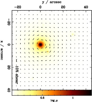
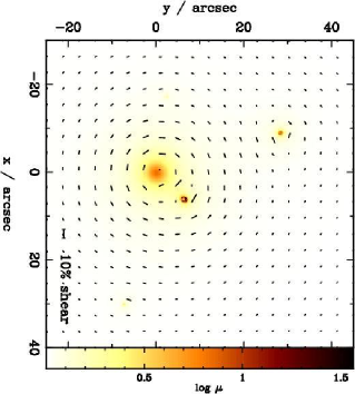
(c)                                                           (d)

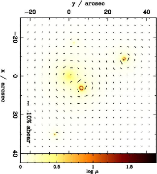
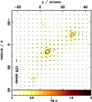
Figure 4: Shear and magnification maps for a typical compact group with 4 member galaxies. The panels show the magnification on the image plane as a grey-scale. The direction and relative magnitude of the shear is indicated by the arrows in each panel. Panel (a) is for a group corresponding to Model A in table 2, panel (b) for a group corresponding to Model B and panel (c) for a group corresponding to Model C. Panel (d) shows the shear and magnification for a group as in Model D, with no halo. In all panels, the source plane redshift is taken to be $z_{\mathrm{s}}=1.0$.

The galaxy substructure is clearly evident in all the shear and magnification maps. However, the figure also illustrates that this substructure is unlikely to be detectable for an individual group; the shear signal is too small. In order to make a positive detection, many groups will have to be stacked. Fig 5 shows the sensitivity of the inner slope of the shear profile for an average of 100 stacked groups with varying group halo to galaxy mass ratio.

Figure 5: The tangential shear averaged over 100 groups for different values of the halo mass: galaxy mass ratio. The total group mass is the same in all cases. The overplotted observational data point is from Hoekstra et al. (2001) for the CNOC2 groups.

The shear signal within 20” varies by about 1 percent, which is once again detectable when averaged over 100 groups. There is however some uncertainty, as we have do not have a priori knowledge of the profile slope and core radius of the intergalactic group halo. A possibility would be to use the X-ray profile, and assume that the same form describes the mass distribution in the halo. Another difficulty arises from the fact that it is necessary to determine the position of the ‘center’ of the group in order to stack the tangential shear signal coherently. If either this determination is inaccurate or the intergalactic halo is off-center from this position, then the measured shear profile will be flatter, leading to a systematic underestimate in the halo mass fraction. An elegant solution to these problems is to add the average tangential shear around each member galaxy. The positions of galaxies can be determined accurately from their light distribution. Furthermore, the slope of the mass profile of the individual galaxies is much better constrained from the studies of individual lenses. Since the constraints on the positions and profiles of the individual galaxies are likely to be tighter, the average shear profile around each of the member galaxies can be related directly to the group halo to galaxy mass ratio. Determining the shape of the average shear profile around a set of galaxies can therefore provide a new, important and feasible way of determining the relative mass fraction in galaxies in different environments. Fig. 6 shows the resulting shear profile around the member galaxies averaged over 100 groups.

Figure 6: The average tangential shear around the individual group members of 100 simulated groups for different halo : galaxy mass ratios. The qualitative behavior is similar to that in Fig. 5; the signal at small radii is strongly dependent on the relative masses of galaxy and group halos. Note that the difference between this plot and the previous one lies in the choice of center around which the shear field is averaged.

Qualitatively, the same effect is seen in both cases (independent of choice of center), a strong correlation between the relative mass distributions and the average value of the shear; however for the case of massive halos, the average shear around group members is significantly reduced at small radii. In the following sections the average shear around the member galaxies, rather than the shear around the ill-defined group center, will be considered.

4.2 Dependence on the density profile of galaxies in the group

The galaxy profile given in eq. 2 has been used extensively and provides a good approximation to the true mass profile of most galaxies. Furthermore, past studies have shown that galaxies have a compact core radii, and as shown in Fig. 2, the observed shear variations with galaxy core radius and ellipticity is expected to be small. The effect of the choice of the form of the galaxy number density profile on the measured shear is shown in Fig. 7.

Figure 7: The average tangential shear around the individual group members of 100 simulated groups for different shapes of the galaxy number density profile, eq. 4. The groups are generated randomly as described in section 2.2 and are all at $z_{\mathrm{l}}=0.3$.

The figure shows that for number density profiles steeper than the modified Hubble-Reynolds law, the average tangential shear at radii of about 30 arcseconds is increased relative to the inner average shear. This is due to an increase in the average mass density both inside the group and around member galaxies for more spatially compact groups.

The analysis presented here mainly concerns the study of small compact groups. We also performed simulations for group scale lengths between 15 and 40 kpc and found that the shear profile does not vary significantly; this is as we expect given that we normalize the mass at a relatively small radius of $100\,\mathrm{kpc}$.

Recently, there has been much discussion about the NFW (Navarro, Frenk & White 1996) density profile – which has been fit successfully in N-body simulations to dark matter halos on a large range of scales from small galaxies to rich clusters. The lensing properties of this profile have been studied recently by (Wright & Brainerd 2000). We explore this density profile for group members in our simulations. The NFW profile has the form,

$$\rho(r)=\frac{\rho_{0}}{r/r_{\mathrm{s}}(1+r/r_{\mathrm{s}})^{2}},$$ (16)

where $r_{\mathrm{s}}$ is a characteristic scale length and $\rho_{0}$ is a central density. The total mass interior to radius $R$ for an NFW profile is

$$M(r)=4\pi\rho_{0}r_{\mathrm{s}}\left(\ln({1+\frac{r}{r_{\mathrm{s}}}})-\frac{r}{r+r_{\mathrm{s}}}\right).$$ (17)

Analytical expressions for the shear can be found in Wright & Brainerd (2000) and Trentham, Möller & Ramirez-Ruiz (2000). The scale lengths for this galaxy model are assigned randomly in exactly the same way as for the PIEMD as described in section 2.2. The total mass inside a radius of $100\,\mathrm{kpc}$ is set to the same value as for the PIEMD. Since the NFW profile is shallower inside $r_{\mathrm{s}}$ and steeper outside that radius as compared with the PIEMD profile, the mass at small radii is larger than that for the equivalent PIEMD. The shear signal is therefore expected to be larger at small radii. Fig. 8 shows the tangential shear around a group in which all the mass components are modeled as NFW profiles.

Figure 8: The average tangential shear around the individual group members of 100 simulated groups for an NFW galaxy and halo profile. The group properties are determined randomly as for Figs. 2-5. All groups are at $z_{\mathrm{l}}=0.3$ and the source redshift $z_{\mathrm{s}}=1.0$.

Results are qualitatively similar to those obtained for the PIEMDs (in Fig. 3). However, the effect on the shear field of shifting mass from the halo to the individual galaxies is much more pronounced due to the larger mass contained at small radii in the NFW: the central value of the shear is even more sensitive to the halo mass to galaxy mass ratio, and the shear at small radii is generally larger.

4.3 Dependence on the redshift distribution of the group members

Uptil now all group members were assumed to lie at the same redshift. For groups that have been selected from a spectroscopic survey with accurate redshift determinations that will indeed be the case. However, it is instructive to investigate any qualitative differences that might arise in the shear profiles due to projection effects. Fig. 9 shows the average shear around member galaxies for three cases:

Figure 9: The average tangential shear around group members of 100 simulated groups for different lens redshifts. Results for projected groups in which the galaxies are at different redshifts are shown along with the results for compact groups at a single redshift of $z_{\mathrm{l}}=0.3$.

(i) in which all member galaxies are at the same redshift; (ii) where half of the ‘member’ galaxies are at a much higher redshift; and (iii) in which the redshift difference is $\Delta z/z\sim 0.2$. As expected, a small redshift difference does not lead to significantly different results, whereas a larger redshift difference, with only part of the apparent group lying at an optimum lens redshift, leads to a decrease in the shear signal by a factor of a few. Note that the shape of the shear profiles is not affected by differences in redshift and that the measured ratio of the tangential shear at small radius to that at large radius is therefore still a good estimator of the relative halo : galaxy mass ratio. However, since the overall shear signal is reduced if galaxies are mistakenly assumed to be part of a group, the total mass in the group is likely to be systematically underestimated.

5 Strong lensing effects

In the previous section we calculated the expected magnitude of the weak lensing signal due to galaxy groups. In the strong lensing regime, there is clear observational evidence for the effect of the group potential. Many of the known lens systems cannot be described accurately by a single lens model and a significant external shear is required in many cases (Kundic et al. 1997a; Keeton, Kochanek & Seljak 1997; Kneib, Cohen & Hjorth 2000). In fact, groups of galaxies are found near many of these systems (Rusin et al. 2000). In general, the presence of a group in the vicinity of a galaxy lens will lead to an external shear contribution to the main lensing potential. The direction and magnitude of this shear will depend strongly on the precise mass distribution within the group and this will affect the image positions, magnifications, time delays and image geometries. This will be important for modeling both the individual lens systems as well as for lens statistics (number of multiple images produced).

5.1 Individual lens systems

A basic consequence of the presence of a group on the lensing behavior of a nearby galaxy is to introduce some external shear. As shown for example by Keeton, Kochanek & Seljak (1997), the effect of this shear is to introduce an effective asymmetry in the potential which affects the image geometries and magnification ratios. In the following we investigate the effect of the details of the mass distribution inside the group which neighbors an individual lensing galaxy.

5.1.1 Magnification and image geometry

(a)                                                           (b)

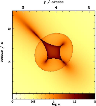
Figure 10: Magnification maps on the source plane for a typical compact group with four member galaxies. The panels are centered on the position of the main lensing galaxy, which has the same properties as galaxy 3 of Model C (tab.2) in both panels. The properties of the group members vary; in the left panel, the group properties are those of Model A; in the right panel, the group properties are those for Model C; Note that the properties of the main lensing galaxy are the same in both panels and the differences in the maps arise solely from the variation of the mass distribution in the surrounding group.

Many of the expected strong lensing properties of particular lens profiles can be determined from the ‘magnification map’ which gives the total magnification as a function of source position on the source plane. The magnification map provides information on the number of images, the calculated magnifications and the lensing cross sections (cf. Möller & Blain 1998). We compute the magnification map on the source plane for the simulated groups using ray tracing; the results for two models are shown in Fig. 10. Comparison of the two panels in Fig. 10 shows qualitatively how the strong lensing properties of a group member depend on the relative masses of the galaxies within the group. The main differences/similarities in the magnification maps are:

1. The area inside the astroid shaped caustic is larger for the model with a more massive group halo. Sources that lie inside the astroid shaped caustics, seen in Fig. 10(a) & (b), are imaged into four magnified images. Therefore, in this particular configuration, the lensing galaxy is more likely to produce quadruple images if it is part of a group with a massive halo than if it is part of a group without such a halo.

2. The astroid shaped caustic line is longer for a more massive group halo. The probability that a small background source is magnified strongly is, to first order, proportional to the length of the caustic. Extended caustics are therefore more likely to produce high-magnifications, and so, in this particular configuration, the lensing galaxy is more likely to produce strongly magnified images if it is part of a group with a massive halo.

3. The area inside the outer, circular caustic that surrounds the astroid shaped caustic, is independent of the mass distribution of the group. Sources that lie outside the area enclosed by this caustic are not multiply imaged, and, therefore, if observational magnification bias is ignored, the total strong lensing cross section is not strongly dependent on the mass distribution of the group.

From this, we conclude that for individual lens systems that have neighboring groups the details of the mass distribution in the group is expected to have a significant effect on the magnifications and image geometries.

5.1.2 Lens modeling and time delays

Many strong gravitational lens systems have been used to estimate the Hubble parameter $H_{0}$ through a measurement of their time delay (e.g. Koopmans et al. 2000). Uncertainties in the derived value of $H_{0}$ are caused mainly by inaccuracies and uncertainties in models for the lensing potential. Many of these lens systems are part of, or lie near, a group (Kundic et al. 1997b), and it is therefore important to quantify the effect of the group on the measured time delay. Once again ray-tracing routines are used to compute the time delays for the various configurations.

Figure 11: The time delay as a function of image separation for the different group models tabulated in Table 2. The curves are for models A, B, C and D with increasing line thickness. As in Fig. 10 the main lensing galaxy has the same properties in all cases (galaxy 3, Model C in Table 2).

Fig. 11 shows the time delay as a function of image separation for the four different group mass distributions listed in Table 2. Despite the fact that the properties of the main galaxy are identical in all three panels, there is a significant variation in the time delay between different group models. The plot shows that the group potential itself has a great effect on the time delay; the presence of a massive group halo leads to smaller maximum image separations and therefore larger time delays. Since $\Delta T\propto H_{0}^{-1}$, this has important consequences for the determination of $H_{0}$ from such systems. For example, for a lens system with image separations of $2"$, we estimate that the value of $H_{0}$ deduced from a time delay of about 80 days will vary from $50\,\mathrm{km\,s^{-1}\,Mpc^{-1}}$, for a 70% halo to $100\,\mathrm{km\,s^{-1}\,Mpc^{-1}}$ for no group halo. Therefore, depending on the relative mass of a group halo, the value of $H_{0}$ may be seriously underestimated if the group halo is not included in the lens modeling.

5.2 Statistical strong lensing

In the following we investigate the effect of the group mass distribution on strong lensing statistics using the ray tracing simulations and a sample of 100 random groups. In each group a single galaxy at position $\vec{r_{\mathrm{l}}}$ is chosen to be the main lensing galaxy and we determine the magnifications, time-delays and image geometries for the lensing galaxy in each group, averaging the results for the whole sample. The groups are generated as described in Sec. 2, except that we set the ellipticities of the individual galaxies $\epsilon=0$ in the interest of computational speed. Our results will not affected by the simplifying assumption that $\epsilon=0$; since non-zero ellipticities introduce only an additional statistical error that is proportional to $\sqrt{N}$, where $N$ is the number of lens systems in the sample.

For each system we obtain statistical information from the image information stored on a grid in the source plane, as described in Sec. 3.1.2. In order to simulate observational selection effects, we also produce one set of results that only includes images with magnification ratios smaller than 20 and separations larger than $0.1"$. We do not include magnification bias explicitly. This makes the results discussed below conservative, as magnification bias will increase the effect of groups on statistical lensing properties, since highly magnified sources are more probable in lens systems with substantial external shear.

5.2.1 Multiplicity of images, image separations and magnification ratios

We determined the image separations and magnification ratios for all image pairs for all 100 groups in the simulated sample. Investigating the statistics of the number of images, we found that changing the mass distribution inside the group had little effect; the cross sections for lensing into three, four and five images varied by less than 10%. This shows that even though image multiplicities of individual systems may be influenced strongly by the particular direction and magnitude of the shear, the average effect for a large sample of stacked lens systems is small.

The maximum image separations depend on the projected mass contained inside the smallest circle that contains all images (Schneider et al. 1992). Therefore, external shear that involves only a contribution to $\gamma$ will not affect the maximum image separations unless the image multiplicities are increased. The presence of a group will affect the maximum image separations only if there is a significant contribution to the mean $\kappa$ from the group.

Figure 12: The distribution of image separations expected for a large sample of strong lens systems. The histograms are obtained by binning the angular separation $\Delta\theta=|\vec{\theta_{\mathrm{A}}}-\vec{\theta_{\mathrm{B}}}|$ for each pair of images of a given source. Each lensing galaxy is at a random position within the group, determined using equation 4. The statistics only include images that are separated by more than $0.1"$ and have a magnification ratio less than 1 : 20.

Fig. 12 shows the distribution of image separations for different group mass distributions for four different choices of the relative position between lensing galaxy and group. The distance of the lensing galaxy from the group center is determined randomly from the distribution given by eq. 4. The figure shows that, as expected, massive group halos lead to slightly larger separations. This effect is in principle detectable, given a sample of 100 appropriate lens systems. However, in practice some additional information is needed to disentangle the degeneracy between a contribution to $\kappa$ due to a separate group halo component and due to a more massive lens galaxy. Fig. 12 also shows the significant effect of selection criteria on lensing statistics. If useful information about the lens population is to be gained from lens statistics the observational selection criteria need to be understood.

The magnification ratio $\mu_{\mathrm{r}}=\mu_{\mathrm{A}}/\mu_{\mathrm{B}}$ for two images $A$ and $B$ is given by eq. 12. In the case $\kappa_{\mathrm{A}}\approx\kappa_{\mathrm{B}}\approx 0$, the magnification ratio can be approximated as $\mu_{\mathrm{r}}=(1-\gamma_{\mathrm{B}}^{2})/(1-\gamma_{\mathrm{A}}^{2})$. If $\vec{\gamma}$ varies significantly over distances of the order of the image separations ($\approx 1$ arcsec), the magnification ratios are expected to be larger than if $\vec{\gamma}$ varies only slightly. Thus, any variation of the external shear due to differences of the mass distribution of the group may change the distribution of magnification ratios.

Figure 13: The magnification ratio distribution expected for a large sample of strong lens systems. The histograms are obtained by binning the magnification ratio for each pair of images of a given source. The positioning of the lens galaxy is random and the line styles are as in Fig. 12.

Fig. 13 shows histograms of the distribution of magnification ratios for different group mass distributions. The figure shows that massive group halos lead to slightly larger magnification ratios, but the effect is small ($<15$%). As in Fig. 12 observational selection effects change the statistics significantly, even for relatively low magnification ratios of $\mu_{\mathrm{r}}\approx 5$.

5.2.2 Effect on the time-delay

Now we assess the effect of the detailed mass distribution on the statistical time-delay of a larger sample of lens systems (note that the time-delay was determined as described in Sec.3.1.2).

Figure 14: The time-delay statistics for different halo masses, from simulations of 100 group systems. The histograms show the fraction of systems with a given time-delay that are expected in a large sample of strong lens systems which are associated with compact groups. The panels (a)-(c) show the results for three different separations between the lensing galaxy and the group center, $\delta\phi$. In panel (d) the distance of the lensing galaxy from the group center is determined randomly from the distribution given by eq. 4.

For each source, the maximum time-delay between image pairs is binned to create the histograms shown in Fig. 14. Panels (a)-(c) show the results for separations $\delta\phi=|\vec{r_{\mathrm{h}}}-\vec{r_{\mathrm{l}}}|$ between the lensing galaxy and the group center at $\vec{r_{\mathrm{h}}}$ of $\delta\phi=5"$, $\delta\phi=10"$ and $\delta\phi=30"$ respectively. In panel (d) the distance of the lensing galaxy from the group center is determined randomly from the distribution given by eq. 4. Strong lens systems in which the main lensing galaxy is associated with a group that contains a massive group halo statistically have larger time-delays, whereas lens systems in groups without a massive halo will have a more strongly peaked distribution of time-delays with a maximum around the corresponding average Einstein radius. Thus, measuring the time-delays of a sample of about 100 lens systems associated with compact groups could provide information on the mass distribution in groups, provided the value of $H_{0}$ is known. If the value of $H_{0}$ is to be deduced from a statistical sample of lens galaxies, care has to be taken to account fully for the presence of groups. If a significant number of lens systems used to determine $H_{0}$ are near groups with massive halos, and this is not taken into account, the value of $H_{0}$ can be underestimated even by upto factors of 2 or more!.

6 Conclusions

Even though velocity dispersions can be measured to constrain the total mass of groups (Mahdavi et al. 2000), the mass distribution inside groups is currently not well known. If additional assumptions about the correlation between X-ray luminosity and mass density are made, details of the dark matter distribution can be obtained from sensitive, high-resolution X-ray images. Only gravitational lensing provides a direct probe of the surface mass density and its spatial distribution. In this paper, we demonstrate using numerical techniques, that weak and strong gravitational lensing can be used to constrain both the total mass and the details of the mass distribution in groups.

In summary, the results for weak lensing properties groups are as follows:

1. The weak lensing shear signal of groups is about 3 per cent, and varies by up to a factor of 2 for different mass distributions. More importantly, the ratio of the tangential shear at small radii to that at larger distances varies by a factor of a few depending on the mass contained in the group halo.

2. This effect is not detectable for individual groups, but if about $100$ groups are stacked, then the shear signal around the individual member galaxies can be determined with sufficient accuracy to distinguish different mass profiles. The stacking of a large number of groups also decreases the noise due to cosmic variance, which is of the same magnitude as the shear signal for individual groups, to a level of about one per cent of the total group signal.

3. Averaging the shear signal around individual group members has many practical advantages; the measured shear at larger radii provides information on the total group mass, whereas the average shear close to the galaxies measures the galaxy mass fraction.

4. The qualitative results (features in radially averaged tangential shear profile) are independent of the form of the number density profile assumed, the halo scale length and possible projection effects. The level of the signal depends on the details of the assumed density profile, halo scale length and redshifts; however, the form of the shear profile as a function of radius remains the same and is determined only by the halo mass fraction.

5. With new instruments, like ACS (Advanced Camera for Surveys) on $HST$ or the $NGST$ (Next Generation Space Telescope), it should be possible to determine the shear to a sufficient accuracy, so that it will be possible to distinguish different group mass distributions. In particular, it should be viable to determine whether groups possess a significant large scale dark halo.

The synopsis of our strong lensing results are:

1. In the strong lensing regime the presence of groups and the mass distribution within the group, can affect the magnification maps and caustic structure significantly for an individual lens in the vicinity. The observed time-delay is particularly sensitive to the details of the mass distribution in the surrounding group. This systematic error needs to be taken into account when making estimates of $H_{0}$ from time-delay measurements.

2. In individual lens systems, the probability of multiple imaging into 3 or more images may be increased in cases where the main lensing galaxy is part of or very close to a group. In particular, lens models which do not take the presence of the group into account are likely to underestimate the cross section for high-image multiplicities.

3. Statistically, the magnification ratio of images with large separations is larger for lensing galaxies that are part of groups with a massive halo.

4. The statistics of time-delays can also be used to constrain the mass distribution in groups; lens systems in groups with a high halo mass fraction will on average have larger time-delays.

Weak and strong gravitational lensing studies can provide important constraints on the mass content and distribution of mass in groups of galaxies.

References

- (1)
- (2) Bartelmann, M., Huss, A., Colberg, J. M., Jenkins, A., Pearce, F. R., 1998, A&A, 330, 1
- (3)
- (4) Bartelmann, M., & Schneider, P., 2001, Phys. Rep., 340, 291
- (5)
- (6) Barton, E., Geller, M., et al., 1996, AJ, 112, 871
- (7)
- (8) Blandford, R. D., Cohen, J., Kundic, T., Brainerd, T., Hogg, D., 1998, AAS Bulletin, Vol. 192, p. 0704
- (9)
- (10) Brainerd, T. G., Blandford, R. D., & Smail, I. R., 1996, ApJ, 466, 623
- (11)
- (12) Clowe, D., Luppino, G. A., Kaiser, N., Gioia, I. M., 2000, ApJ, 539, 540
- (13)
- (14) Cohn, J. D., Kochanek, C. S., McLeod, B. A. & Keeton, C. R., 2001, ApJ, 554, 1216
- (15)
- (16) de Carvalho, R. R., & Djorgovski, S. G., 1995, BAAS, 187:53.02
- (17)
- (18) Ettori, S., & Fabian, A. C., 2000, MNRAS, 317, L57
- (19)
- (20) Fischer, P., 1999, AJ, 117, 2024
- (21)
- (22) Geiger, B., & Schneider, P., 1999, MNRAS, 302, 118
- (23)
- (24) Girardi, M., & Giuricin, G., 2000, ApJ, 540, 45
- (25)
- (26) Helsdon, S. F., & Ponman, T. J., 2000, MNRAS, 315, 356
- (27)
- (28) Hickson, P., 1982, ApJ, 255, 382
- (29)
- (30) Hickson, P., Kindl, E., & Huchra, J. P., 1988, ApJ, 329, L65
- (31)
- (32) Hickson, P., Mendes de Oliviera, C., Huchra, J. P., & Palumbo, G.G., 1992, ApJ, 399, 353
- (33)
- (34) Hoekstra, H., et al., 2001, ApJ, 548, L5
- (35)
- (36) Hoekstra, H., Franx, M., & Kuijken, K., 2000, ApJ, 532, 88
- (37)
- (38) Hoekstra, H., Franx, M., Kuijken, K., & Squires, G., 1998, ApJ, 504, 636
- (39)
- (40) Humason, M. L., Mayall, N. U., & Sandage, A. R., 1956, AJ, 61, 97
- (41)
- (42) Kaiser, N., 1995, ApJ, 439, L1
- (43)
- (44) Kassiola, A., & Kovner, I., 1993, ApJ, 417, 450
- (45)
- (46) Keeton, C. R., Kochanek, C. S., & Seljak, U., 1997, ApJ, 482, 604
- (47)
- (48) Kneib, J., Cohen, J. G., & Hjorth, J., 2000, ApJ, 544, L35
- (49)
- (50) Koopmans, L. V. E., de Bruyn, A. G., Xanthopoulos, E., & Fassnacht, C. D., 2000, A&A, 356, 391
- (51)
- (52) Kundic, T., Hogg, D. W., Blandford, R. D., Cohen, J. G., Lubin, L. M., & Larkin, J. E., 1997a, AJ, 114, 2276
- (53)
- (54) Kundic, T., Turner, E. L., Colley, W. N., Gott, J. R. I., Rhoads, J. E., Wang, Y., Bergeron, L. E., Gloria, K. A., et al., 1997b, ApJ, 482, 75
- (55)
- (56) Mahdavi, A., Böhringer, H., Geller, M. J., & Ramella, M., 2000, ApJ, 534, 114
- (57)
- (58) Markevitch, M., Vikhlinin, A., Forman, W. R., & Sarazin, C. L., 1999, ApJ, 527, 545
- (59)
- (60) Mellier, Y., 1999, ARA&A, 37, 127
- (61)
- (62) Möller, O., & Blain, A. W., 1998, MNRAS, 299, 845
- (63)
- (64) Möller, O., & Blain, A. W., 2001, MNRAS, in press
- (65)
- (66) Mulchaey, J. S., & Zabludoff, A. I., 1998, ApJ, 496, 73
- (67)
- (68) Natarajan, P., & Kneib, J., 1996, MNRAS, 283, 1031A
- (69)
- (70) Natarajan, P., & Kneib, J., 1997, MNRAS, 287, 833A
- (71)
- (72) Natarajan, P., Kneib, J., Smail, I., & Ellis, R. S., 1998, ApJ, 499, 600
- (73)
- (74) Navarro, J., Frenk, C. S., & White, S. D. M., 1996, ApJ, 462, 563
- (75)
- (76) Ponman, T.J., Allan, D. J., Jones, L. R., et al., 1995, Nature, 369, 462
- (77)
- (78) Press, W. H., & Schechter, P., 1974, ApJ, 187, 425
- (79)
- (80) Press, W. H., et al., 1988, Numerical Recipes, Cambridge University Press, Cambridge.
- (81)
- (82) Ramella, M., Pisani, A., & Geller, M. J., 1997, AJ, 113, 483
- (83)
- (84) Ramella, M., Zamorani, G., Zucca, E., Stirpe, G. M., Vettolani, G., et al., 1999, A&A, 342, 1
- (85)
- (86) Schneider, P., Ehlers, J. ., & Falco, E. E., 1992, ”Gravitational Lenses”. Springer-Verlag Berlin Heidelberg New York.
- (87)
- (88) Schneider, P., van Waerbeke, L., Jain, B., Kruse, G., 1998, MNRAS, 296, 873
- (89)
- (90) Schramm, T., 1990, A&A, 231, 19
- (91)
- (92) Trentham, N., Möller, O., Ramirez-Ruiz, E., 2001, MNRAS, 322, 658
- (93)
- (94) Wambsganss, J., Cen, R., & Ostriker, J. P., 1998, ApJ, 494, 29
- (95)
- (96) Williams, B. A., & Rood, H. J., 1987, ApJ Supp., 63, 265
- (97)
- (98) Wright C. O., & Brainerd T. G., 2000, ApJ, 534, 34
- (99)
- (100) Zabludoff, A., 2001, Proc. of conf. on Gas and Galaxy Evolution, ASP Conf. Series, in press, astro-ph/0101214
- (101)
- (102) Zabludoff, A., & Mulchaey, J., 1998, ApJ, 496, 39
- (103)
- (104) Zabludoff, A., & Mulchaey, J., 2000, ApJ, 539, 136
- (105)