Chandra discovery of extended non-thermal emission in 3C 207 and the spectrum of the relativistic electrons

We report on the Chandra discovery of large scale non–thermal emission features in the double lobed SSRL quasar 3C 207 (z=0.684). These are: a diffuse emission well correlated with the western radio lobe, a bright one sided jet whose structure coincides with that of the eastern radio jet and an X–ray source at the tip of the jet coincident with the hot spot of the eastern lobe. The diffuse X–ray structure is best interpreted as inverse Compton (IC) scattering of the IR photons from the nuclear source and provides direct observational support to an earlier conjecture (Brunetti et al., 1997) that the spectrum of the relativistic electrons in the lobes of radio galaxies extends to much lower energies than those involved in the synchrotron radio emission. The X–ray luminous and spatially resolved knot along the jet is of particular interest: by combining VLA and Chandra data we show that a SSC model is ruled out, while the X–ray spectrum and flux can be accounted for by the IC scattering of the CMB photons (EIC) under the assumptions of a relatively strong boosting and of an energy distribution of the relativistic electrons as that expected from shock acceleration mechanisms. The X–ray properties of the hot spot are consistent with a SSC model. In all cases we find that the inferred magnetic field strength are lower, but close to the equipartition values. The constraints on the energy distribution of the relativistic electrons, imposed by the X–ray spectra of the observed features, are discussed. To this aim we derive in the Appendices precise semi–analytic formulae for the emissivities due to the SSC and EIC processes.

1 Introduction

A full understanding of the energetics and energy distribution of relativistic particles in radio jets and lobes of radio galaxies and quasars is of basic importance for a complete description of the physics and time evolution of these sources. It is assumed that the relativistic electrons in powerful radio sources are channeled into the jet and re–accelerated both in the jet itself (e.g., in the knots) and in the radio hot spots, which mark the location of strong planar shocks formed at the beam head of a supersonic jet (e.g. Begelman, Blandford, Rees, 1984). Then particles diffuse from the hot spots forming the radio lobes.

X–ray observations of both compact features and lobes of radio sources are of basic importance in constraining the energetics and spectrum of the relativistic electrons and possibly their evolution.

Until the advent of Chandra, only a few examples of X–ray emission from radio jets and hot spots were available (e.g. Cygnus A: Harris, Carilli, Perley, 1994; 3C 120: Harris et al., 1999; 3C 273: Röser, et al., 2000; M87: Neumann, et al., 1997). It has been immediately clear that the detected emission is of non–thermal origin with the best interpretation provided by synchrotron and SSC mechanisms under minimum energy conditions (equipartition between electron and magnetic field energy densities).

X–ray emission from the radio lobes has been discovered by ROSAT and ASCA in a few nearby radio galaxies, namely Fornax A (Feigelson et al.1995; Kaneda et al.1995; Tashiro et al.2001) and Cen B (Tashiro et al., 1998), with the best interpretation provided by the IC scattering of the Cosmic Microwave Background (CMB) photons. In addition combined ROSAT PSPC, ASCA and ROSAT HRI observations of the powerful radio galaxy 3C 219 have also shown the presence of extended X–ray emission within $\sim 80$ kpc distance from the nucleus which is interpreted as IC scattering of the IR photons from a hidden quasar (Brunetti et al.1999). In general these observations are complicated due to the weak X–ray brightness and relatively low count statistics, however, the magnetic field strengths estimated from the combined IC and synchrotron radio fluxes are within a factor of $\sim 3$ consistent with the equipartition values. Up to now no clear evidence of extended non–thermal emission from radio loud quasars has been found.

Likewise Chandra is providing a significant progress on the study of the X–ray emission from jets and hot spots (Chartas et al., 2000; Harris et al., 2001; Wilson, et al., 2000; Schwartz et al., 2000; Wilson, et al., 2001; Hardcastle, et al., 2001a,b; Pesce et al.2001). Although the analysis of the increasing number of successful detections of X–ray emission from compact hot spots and jets has confirmed the non–thermal nature of the X–rays from these sources, it is not clear whether the SSC and synchrotron model can provide or not a general interpretation of the data (e.g. Harris 2000). One of the most striking cases is the X–ray jet of PKS 0637$-$752, where the SSC mechanism can only provide a flux about 2 orders of magnitude below the observed (Chartas et al., 2000). A viable explanation is based on the assumption that even far from the core the jet has a relatively high relativistic bulk motion (Celotti, et al., 2001; Tavecchio et al., 2000) so that the CMB photons can be efficiently up–scattered into the X–ray band (EIC model).

Chandra is the first X–ray observatory able to well resolve the radio lobes of powerful and relatively distant radio galaxies and quasars; thus, for the first time it is now possible to well separate the non–thermal lobe emission in these objects from the surrounding cluster emission. An example is provided by the radio galaxy 3C 295 where the diffuse X–ray emission from the radio lobes in excess to that of the surrounding cluster has been best interpreted via IC scattering of nuclear photons under equipartition conditions (Brunetti et al., 2001).

In this paper we report the Chandra observation of the radio loud quasar 3C 207. A powerful one sided X–ray jet, coincident with the radio one is discovered whereas, in the opposite direction, extended X–ray emission coincident with the western radio lobe is also detected. The X–ray jet is characterized by two knots which coincide with the main radio knot and with the western hot spot. In Sects.2.2 and 2.3 we report the radio VLA and Chandra results, respectively. In Sect.3.2 we report the interpretation and modeling of the results obtained for the lobe emission, while the interpretation of the western knot and hot spot is reported in Sects.3.3 and 3.4, respectively. To model these results we make use of the electron energy distributions obtained in the framework of shock acceleration theory and of general equations for SSC and EIC processes. A simple analytic model for electron shock acceleration is worked out in Sect.3.1, whereas the general SSC and EIC equations are derived in the Appendices. The discussion of the results and conclusions are reported in Sect.4.

$H_{0}=50$ km s^-1 Mpc^-1 and $q_{0}=0.5$ are assumed throughout: 1 arcsec corresponds to 7.9 kpc at the redshift of 3C 207.

2 Target and data analysis

2.1 3C 207

The powerful radio source 3C 207 is identified with a quasar at a redshift of z=0.684. The integrated radio spectrum is relatively steep, $\alpha\simeq 0.9$ ($F(\nu)\propto\nu^{-\alpha}$), between 150–750 MHz (Laing et al., 1983), whereas it flattens at higher frequencies ($\alpha\simeq 0.64$ and 0.43 around 2.5 and 40 GHz, respectively; Herbig & Readhead 1992) where the nuclear component dominates.

Bogers et al.(1994, and ref. therein) obtained detailed radio images at 1.4 and 8.4 GHz. The radio source is relatively compact with an extension of about 10 arcsec. At low radio frequencies a relatively high brightness double lobed structure appears; the radio flux and extension of the two lobes are similar. At high frequency 3C 207 shows a prominent radio jet pointing in the direction of the eastern lobe.

The combination of powerful radio lobes and relatively small angular extension makes this source a good candidate to study the IC scattering of the nuclear photons in the radio lobes. In addition, the high spatial resolution of Chandra allows to well resolve the luminous radio jet in the X–ray band and to obtain spectral information on both the X–ray jet and lobes.

2.2 The archive radio Data

With the aim to compare the radio and X-ray morphology on the arcsec-scale, and derive the radio spectral indices of the extended emission and compact components, we requested and re-analyzed some of the VLA archive data (Tab.1) of 3C 207.

Table 1: VLA Data Archive

Proj Code	Date	$\nu$(MHz)	Array	TOS(s)
AL280	Dec-13-1992	1415/1665	A	3490
AL280	Dec-13-1992	14915/14965	A	540
AL113	Jul-12-1986	4835/4885	B	670
AB796	Nov-08-1996	8435/8475	A	16410
AB796	Mar-04-1997	8435/8485	B	1490

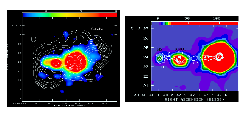
Figure 1: The Chandra 0.2–10 keV image (color) is superimposed on the VLA 1.4 and 15 GHz isophotes (left and right panel respectively). A $\simeq 0.9$ arcsec shift has been applied to match the X–ray and radio peaks. Left Panel: The Chandra image is obtained with a smoothing ($\sigma$=1.8 pixels) of a subsampled (0.25 arcsec square pixels, i.e. binned at 0.5 original pixels) image. The 1.4 GHz radio contours are: $1\cdot 10^{-3}\times$ (-1, 1, 2, 4, 8, …) Jy/beam; the FWHM of the beam is 1.4$\times$1.4 arcsec and the flux peak in the image is 0.315 Jy/beam; this resolution is comparable to that of the X–ray image. Right Panel: Close up of the X–ray and radio jet. The Chandra image is obtained with a smoothing ($\sigma$=2 pixels) of a subsampled (0.1 arcsec square pixels, i.e. binned at 0.2 original pixels) image. The 15 GHz radio contours are: $8\cdot 10^{-4}\times$ (-1, 1, 4, 8, 16..) Jy/beam; the FWHM of the beam is 0.25$\times$0.25 arcsec and the flux peak in the image is 0.757 Jy/beam.

Table 2: X–ray and radio spectral analysis

Component	$N_{\rm H}$	$\Gamma$	Norm	$\chi^{2}$/dof	kT	$\chi^{2}$/dof	$\alpha_{1.4}^{4.8}$	$\alpha_{4.8}^{8.6}$	$\alpha_{8.6}^{14.9}$
	($10^{20}$cm-2)		(${{10^{-6}{\rm ph}}\over{{\rm cm}^{2}\,{\rm s}\,{\rm keV}}}$)		(keV)
Nucleus	16.5$\pm$3.5	$1.22_{-0.05}^{+0.06}$	$163_{-12}^{+9}$	201.2/182	…	…	…	…	…
Knot	5.4 (f)	1.23${}^{+0.33}_{-0.29}$	4.6$\pm$0.1	11.4/10	80($>$10.4)	11.7/10	0.78$\pm$0.06	0.88$\pm$0.12	1.83(1.09)$\pm$0.13
Hot Spot	5.4 (f)	1.7${}^{+1.3}_{-0.7}$	1.3$\pm$0.5	…	…	…	0.80$\pm$0.06	0.88$\pm$0.12	1.43(1.17)$\pm$0.13
C–lobe	5.4 (f)	1.46${}^{+0.36}_{-0.34}$	4.5$\pm$0.1	9.6/9	15($>$5.7)	9.4/9	0.92$\pm$0.06	0.89$\pm$0.12	…

Standard data reduction was done using the National Radio Astronomy Observatory (NRAO) AIPS package. We used the 1.4, the 4.8 and 8.4 GHz B array data to obtain “low resolution” images with a circular restoring beam of 1.4 arcsec. The self-calibration and imaging procedure at each frequency was performed using only the uv-points within a common minimum and maximum baseline. These images allow to derive morphological and spectral information of the main jet and of the extended lobe emission. The 8.4 GHz A array and the 14.9 GHz data were used to obtain “high resolution” images with a circular restoring beam of 0.25 arcsec. The self-calibration and imaging procedure at each frequency were performed using only the uv-points within a common minimum and maximum baseline. The “high resolution” image (Fig.1) resolves the radio jet in three main components: an innermost knot at $\sim$2 arcsec from the nucleus, a second knot at $\sim$4 arcsec from the nucleus and a hot spot at the end of the jet. Since Chandra cannot separate the innermost knot from the luminous nuclear source, in the following we focalize on the knot at 4 arcsec distance and on the hot spot.

The radio spectra of the knot and of the hot spot are relatively steep with a similar spectral index ($\alpha\sim 0.8-0.9$, see Tab.2). Although higher frequencies ($\geq 100$ GHz) radio observations would be necessary to better describe the spectrum of both knot and hot spot, we find some evidence of a high frequency spectral steepening. From an inspection of the radio fluxes (UMRAO Database Interface, http://www.astro.lsa.umich.edu/obs/radiotel/umrao.html) at the epochs of the archive data (Tab.1) we find that 3C 207 shows moderate flux variability at a level of $\leq 40\%$ at 15 GHz, probably induced by the nuclear component, whereas the variability at lower frequencies (e.g., 4.8 GHz), where the contribution of the nuclear component is expected to be slightly lower, is reduced to $\leq 20$%. This evidence, combined with the lack of synchrotron self absorption in the spectra of both knot and hot spot, suggests that for these components the spectral variability is not important and that the derived spectral indices (Tab.2) are robust.

Figure 2: The Chandra spectrum of the nucleus of 3C 207. The fitted model is a power law ($\Gamma=1.22$) component absorbed by a column density $N_{\rm H}=1.65\times 10^{21}$cm^-2, plus a narrow gaussian iron line component centered at 6.87 keV (rest frame) with a rest frame equivalent width of 150 eV (dashed). A reflection component from a Seyfert–like spectrum (dot–dashed) is also added to the model (see text).

A visual inspection of the 1.4–8.4 GHz spectral index image of the western lobe does not show clear spatial trends (steepening or flattening) about the average value $\alpha\sim 0.9$, whereas at higher frequencies it is difficult to obtain spectral information due to the lack of the adequate short baselines. This may indicate a rather constant electron spectrum ($\delta\sim 2.8$; $N(\gamma)\propto\gamma^{-\delta}$) in the radio volume. However, as 3C 207 is classified as a quasar, its radio axis is seen at a relatively small angle with the line of sight and projection effects may be important. A relatively constant spectral index in the lobes might derive from the mixing of regions with flatter and steeper spectrum intercepted by the line of sight. As in the case of the global (i.e. spatially unresolved) spectrum of radio galaxies, the mixing of different spectra in 3C 207 can be fitted with a synchrotron continuous injection model (e.g., Kardashev 1962). We find that a continuous injection model with a flat injected spectrum, $\delta\sim 2$, fits the spectrum of 3C 207 if the break energy (i.e. the highest energy of the oldest electrons in the radio volume) is $\gamma_{\rm b}<2\times 10^{3}$ (assuming typical magnetic field strengths).

2.3 Chandra Data

The quasar 3C 207 was observed for 37.5 ksec with the Chandra X–ray observatory on 2000 November 4. The raw level 1 data were re–processed using the latest version (CIAO2.1) of the CXCDS software. The target was placed about 40” from the nominal aimpoint of the chip 7 (S3) in ACIS–S and thus the on–axis point spread function applies. The lightcurve of the full chip shows evidence for particle background flares in the detector during the last part of the observation. The high background times were filtered out leaving about 30 ksec of useful data which were used in the spectral analysis described below.

Inspection of the X–ray image (Fig.1) shows several immediately apparent features: a bright pointlike source coincident with the radio nucleus, enhanced diffuse emission in the direction of the western counter–lobe (C–lobe) and extended emission in the direction of the radio jet concentrated in two relatively bright X–ray knots. These X–ray knots are spatially coincident with one of the radio knots and with the eastern hot spot. X–ray spectra have been extracted using appropriate response and effective area functions. The spectral data have been grouped into bins with a minimum of 20 counts for the nucleus and 15 counts for the X–ray knot associated with the innermost part of the jet and for the extended emission in the opposite direction. We also examined the spectrum of the X–ray hot spot but with about 40 counts we can only obtain rough spectral information. The nuclear spectrum is well fitted by a single absorbed power law (Fig.2, Tab.2). The excellent counting statistic allowed to obtain stringent constraints on the spectral parameters. The power law slope is extremely flat $\Gamma$ = 1.22$\pm$0.06 while the best fit absorption column density is significantly higher than the Galactic value in the direction of 3C 207 ($N_{\rm H}$ = 5.4 $\times$ 10²⁰ cm^-2, Elvis et al. 1989). Fixing the column density at the Galactic value and adding an intrinsic absorber at the source redshift the best fit $N_{\rm H}$ value is (1.65$\pm$0.35) $\times$ 10²¹ cm^-2. There is also evidence of excess emission around 4 keV. The addition of a narrow gaussian iron line improves the fit at the 98% confidence level (according to the F–test). It is interesting to note that the best fit line energy of 6.87$\pm$0.05 keV in the rest frame (the error is at the 90% confidence level for one parameter) strongly suggest the presence of a highly ionized gas in the nucleus of 3C 207. The observed equivalent width of 91$\pm$50 eV corresponds to 153$\pm$84 eV rest frame. Relatively strong iron lines are common among Seyfert galaxies and and low luminosity radio–quiet quasars while they are rarely observed in radio loud objects (Cappi et al. 1997). A likely explanation is that the beamed non–thermal component overshines the accretion disk emission. In order to model the Seyfert–like and beamed non–thermal contributions a reflection component from a Seyfert–like steep power law (fixed at $\Gamma$=1.9) plus a narrow Gaussian iron line have been added to the flat power law non–thermal spectrum. Although poorly constrained we obtained a good fit to the data with a reflection normalization R $\simeq$ 0.85 (where R= $\Omega$/2$\pi$ and $\Omega$ is the solid angle irradiated by the X–ray source). It is interesting to note that similar results have been recently reported by Reeves et al. (2001) from Newton–XMM observations of the high redshift ($z=3.104$) radio–loud quasar PKS 0537$-$286. In their case, however, the iron line strength implies a much weaker reflection component (R $\simeq$ 0.2) possibly indicating a larger non–thermal beamed contribution as also indicated by the very flat radio synchrotron spectrum of this object.

Figure 3: Confidence contour map pf the photon index, $\Gamma$, as a function of the column density, $N_{\rm H}$, in the case of the knot. The reported contours are at 68, 90 and 99 % confidence level. The Galactic column density is $5.4\times 10^{20}$cm^-2.

Figure 4: The Chandra 0.5–5 kev spectrum of the extended emission projected on the western radio lobe (C–lobe) is compared with a thermal model with 0.3 solar metallicity and ${\rm kT}$=4 keV.

The spectral parameters of the non–nuclear extended components are reported in Table 2. In all the cases a relatively flat power law, with the absorption fixed at the Galactic value, does provide an acceptable description of the data. We have evaluated the influence of background subtraction on the derived spectral parameters using different extraction regions over the detector. The Chandra background is always extremely low and has a negligible effect on the spectral parameter estimation. Their uncertainty is dominated by the counting statistics; in Fig.3 we report the confidence contour map of the photon index and column density in the case of the knot. An equally good description of the data, from the statistical point of view, is obtained using a thermal model with abundances fixed at 0.3 solar. It is important to point out that although the quality of the data is not such to discriminate between the two options (power–law and thermal) the derived best fit temperatures are 15 keV (${\rm kT}>5.7$ keV at 90% conf. level; Fig.4) and 80 keV (${\rm kT}>10.4$ keV at 90% conf. level) for the C–lobe and the bright knot respectively. The relatively high temperature requested to fit the C–lobe spectrum excludes the possibility that a cooling flow from a surrounding low brightness X–ray cluster can significantly contribute to this emission. Alternatively, one may wonder that the C–lobe emission is the core region of a surrounding X–ray cluster. From the luminosity–temperature correlation (e.g., Arnaud & Evrard 1999) one has that thermal emission from a hot cluster (with ${\rm kT}>6$ keV) would provide a luminosity $>10^{45}$erg s^-1. However, we find that the 0.1–10 keV luminosity in excess to the core and jet emission (calculated in a circular region of 200 kpc radius) is only $\sim 8-10\times 10^{43}$erg s^-1 depending on the assumed X–ray spectrum and background. In addition most of this luminosity ($\sim 6-7\times 10^{43}$erg s^-1) is produced in the C–lobe region where the morphology of the X–ray counts is similar to the radio brightness distribution. We conclude that although the presence of a low brightness surrounding cluster cannot be excluded, the great majority of the C–lobe X–ray counts are emitted by a non–thermal process.

3 Interpretation of the data

As discussed in the previous Section the Chandra spectra and morphology of both the lobe–like and jet–like features are not consistent with a thermal scenario. An important finding is that the radio and the X–ray spectra are different, with the X–ray spectra sistematically flatter than the radio ones. This is not in contrast with a non–thermal scenario. Indeed, X–rays produced by IC or SSC processes may select portions of the relativistic electron spectrum quite different from those responsible of the synchrotron radio emission.

In order to explain the observed X–ray properties of 3C 207 we have worked out the spectrum of the relativistic electrons under the very simple assumptions of the standard scenario in which the particles are accelerated/reaccelerated by strong shocks taking place in the compact regions of the radio sources, i.e. hot spots and knots in the radio jets (e.g., Meisenheimer et al., 1997 and ref. therein).

In the framework of shock acceleration theory only particles with Larmor radii larger than the thickness of the shock are actually able to feel the discontinuity at the shock. The shock thickness is of the order of the Larmor radius of thermal protons, so that a cut–off at lower energies is formed in the accelerated spectrum (e.g. Eilek & Hughes 1990, and ref. therein). The presence of such a cut–off should be taken into account when low energy electrons contribute to the emitted X–ray spectra via the IC process. The presence of Coulomb losses would further contribute to the flattening of the electron spectra at lower energies (e.g., Sarazin 1999 and ref. therein), but here they are not considered for simplicity as the basic picture would not change.

The readers not interested in the details can skip sub–section 3.1 (referring to Fig.5) and go directly to sub–sections 3.2 and 3.3 where the expected lobe and jet emissions are discussed.

3.1 The spectrum of the relativistic electrons

We assume a simplified two steps scenario :

a) relativistic electrons, continuously injected in the knots and hot spots with a power law spectrum, are accelerated/re–accelerated in the shock regions subject to radiative losses, thus the final spectrum is given by the competition between acceleration and loss mechanisms;

b) the accelerated electrons diffuse from the shock regions and continuously fill a post–shock region where older electrons are mixed with those more recently injected. In this region electrons are subject to radiative losses only.

Following Kirk et al.(1998), we assume that electrons are injected and reaccelerated by Fermi I – like processes in the shock region from which they typically escape in a time $T_{\rm es}$.

The particle energy distribution, ${\cal N}(\gamma)$, can be obtained by solving the equation of continuity (e.g. Kardashev 1962) with a time–independent approach :

$${d\over{d\gamma}}\left[{\cal N}(\gamma)\right]{{d\gamma}\over{dt}}+{\cal N}(\gamma)\left[{{d^{2}\gamma}\over{d\gamma dt}}+{1\over{T_{\rm es}}}\right]-{{\rm Q}}(\gamma)=0$$ (1)

where $d\gamma/dt=-\beta\gamma^{2}+\chi_{\rm a}\gamma$ ($\chi_{\rm a}$ and $\beta$ the acceleration and radiative losses coefficient, respectively) and $Q$ is the particle injection rate. The resulting total electron spectrum for a continuous injection represented by a truncated power law ${{\rm Q}}(\gamma)={{\rm Q}}\gamma^{-s}$ ($\gamma<\gamma_{*}$) is :

$${\cal N}(\gamma)={{{{\rm Q}}}\over{\chi_{\rm a}}}\left(1-{{\gamma}\over{\gamma_{\rm c}}}\right)^{-\alpha_{-}}\gamma^{-\alpha_{+}}\int_{\gamma_{\rm low}}^{\tilde{\gamma}}{{x^{\alpha_{+}-(1+s)}}\over{\left[1-{{x}\over{\gamma_{\rm c}}}\right]^{1-\alpha_{-}}}}dx$$ (2)

where $\gamma_{\rm low}$ is the minimum energy of the electrons that can be accelerated by the shock, $\tilde{\gamma}=\min\left(\gamma_{*}\,\gamma\right)$, $\alpha_{+}=1+[\chi_{\rm a}T_{\rm es}]^{-1}$, $\alpha_{-}=1-[\chi_{\rm a}T_{\rm es}]^{-1}$, and the high energy cut–off $\gamma_{\rm c}=\chi_{\rm a}/\beta$ is given by the ratio between gain and loss terms. We notice that the slope of the electron spectrum for $\gamma>\gamma_{*}$ does not depend on the spectrum of the electrons injected in the shock. In the following we restrict ourself to the case $s=\alpha_{+}$ and $\chi_{\rm a}\sim T_{\rm es}^{-1}$ so that $\alpha_{-}=0$, $\alpha_{+}=2$ and the spectral shape is that provided by the classical strong diffusive shock acceleration (e.g. Heavens & Meisenheimer 1987, and ref. therein).

The post–shock region is continuously supplied by the electron spectrum given by Eq.2 whose time evolution due to radiative losses (an approximatively constant magnetic field strength $B$ is assumed) is obtained by solving the time–dependent continuity equation :

$${{\partial{{\cal N}}(\gamma,t)}\over{\partial t}}=-{{\partial}\over{\partial\gamma}}\left[{{d\gamma}\over{dt}}{{\cal N}}(\gamma,t)\right]$$ (3)

so that

$${{\cal N}}(\gamma,t)={{{{\rm Q}}\,\,{{\rm C}}}\over{\chi_{\rm a}}}\gamma^{-2}\int_{\gamma_{\rm low}}^{{\tilde{\gamma}(t)}}x^{-1}\left[1-{{x}\over{\gamma_{\rm c}}}\right]^{-1}dx$$ (4)

where ${\rm C}\sim 1/T_{\rm es}$ provides for the conservation of the flux of the electron number across the shock region, and

$$\tilde{\gamma}(t)={\rm min}\left\{\gamma_{*}\,\,,\,\,{{\gamma}\over{1-\gamma\beta t}}\right\}$$ (5)

Figure 5: A representative spectrum of the accelerated relativistic electrons is reported with the relevant parameters indicated in the panel : the largest energy of the electrons injected in the post–shock region ($\gamma_{\rm c}$), the largest energy of the oldest electrons in the considered volume ($\gamma_{\rm b}$), the largest energy of the electrons injected in the shock region ($\gamma_{*}$), and the lower energy of the electrons accelerated by the shock ($\gamma_{\rm low}$).

Finally, in a post–shock region with size determined by the diffusion length of the particles in the largest considered time T, the volume integrated spectrum of the electron population, $N(\gamma)$, is given by the sum of all the injected electron spectra, i.e. it is obtained by integrating Eq.4 over the time interval 0–T. The solution is given by the following three cases covering different portions of the energy spectrum :

$\bullet$ $\gamma>\gamma_{*}$

$$N(\gamma)={{{\rm Q}\,C}\over{\chi_{\rm a}\beta}}\gamma^{-2}{\rm ln}\left({{1-\gamma_{\rm low}/\gamma_{\rm c}}\over{1-\gamma_{*}/\gamma_{\rm c}}}\times{{\gamma_{*}}\over{\gamma_{\rm low}}}\right)T_{\gamma}$$ (6)

$\bullet$ $\gamma<\gamma_{*}$ and $T_{\gamma}>\gamma^{-1}(1-\gamma/\gamma_{*})$

$$N(\gamma)={{{\rm Q}\,C}\over{\chi_{\rm a}\beta}}\gamma^{-2}\times\{{\rm ln}\left({{1-\gamma_{\rm low}/\gamma_{\rm c}}\over{1-\gamma_{*}/\gamma_{\rm c}}}\times{{\gamma_{*}}\over{\gamma_{\rm low}}}\right)T_{\gamma}+$$

$${1\over{\gamma}}(1-{{\gamma}\over{\gamma_{\rm c}}})\left[{\rm ln}\left({{\gamma}\over{\gamma_{*}}}-{{\gamma}\over{\gamma_{\rm c}}}\right)-{\rm ln}\left(1-{{\gamma}\over{\gamma_{\rm c}}}\right)\right]+$$

$${1\over{\gamma}}\left(1-{{\gamma}\over{\gamma_{*}}}\right)\}$$ (7)

$\bullet$ $\gamma<\gamma_{*}$ and $T_{\gamma}<\gamma^{-1}(1-\gamma/\gamma_{*})$

$$N(\gamma)={{{\rm Q}\,C}\over{\chi_{\rm a}\beta}}\gamma^{-2}\times\{T_{\gamma}\left[1+{\rm ln}\left({{\gamma_{\rm c}/\gamma_{\rm low}-1}\over{{{\gamma_{\rm c}}\over{\gamma}}-1-\gamma_{\rm c}T_{\gamma}}}\right)\right]+$$

$${1\over{\gamma}}\left(1-{{\gamma}\over{\gamma_{\rm c}}}\right)\left[{\rm ln}\left(1-{{\gamma}\over{\gamma_{\rm c}}}-\gamma T_{\gamma}\right)-{\rm ln}\left(1-{{\gamma}\over{\gamma_{\rm c}}}\right)\right]\}$$ (8)

where

$$T_{\gamma}=\cases{(\gamma_{\rm c}/\gamma_{\rm b}-1)/\gamma_{\rm c}\,\,\,\,\,\,\,\,\,\,\,\,\,\,{\rm for}\,\,\,\,\,\gamma<\gamma_{\rm b}\cr(1-\gamma/\gamma_{\rm c})/\gamma\,\,\,\,\,\,\,\,\,\,{\rm for}\,\,\,\,\,\gamma_{\rm b}<\gamma<\gamma_{\rm c}\cr 0\,\,\,\,\,\,\,\,\,\,\,\,\,\,\,\,\,\,\,\,\,\,\,\,\,\,\,\,\,\,\,\,\,\,\,\,\,\,\,\,{\rm for}\,\,\,\,\,\gamma>\gamma_{\rm c}\cr}$$ (9)

and $\gamma_{\rm b}=\gamma_{\rm c}/(1+\gamma_{\rm c}\beta T)$ is the highest energy of the oldest electrons in the volume being considered.

In Fig.5 we show a representative electron energy distribution obtained from Eqs.(6–8). The shape of the obtained spectrum depends on the energy region: around each one of the relevant values of the electron energy ($\gamma_{\rm low}$, $\gamma_{*}$, $\gamma_{\rm b}$ and $\gamma_{\rm c}$) corresponds a break in the spectral distribution. Under the condition $\gamma_{\rm low}<<\gamma_{*}<<\gamma_{\rm b}$, at intermediate energies, for $\gamma_{*}<\gamma<\gamma_{\rm b}$, the slope approaches to $\delta\simeq 2$ (as in the standard diffusive acceleration from strong shocks), at higher energies, for $\gamma>\gamma_{\rm b}$, it approaches to $\delta\simeq 3$ up to a sharp cut–off around $\gamma\sim\gamma_{\rm c}$ (as in the standard diffusive acceleration from strong shocks including radiative losses). In addition at lower energies, for $\gamma<\gamma_{*}$ (i.e. the largest injected energy), the spectrum gradually flattens ($\delta<2$) and a low energy cut–off is formed around $\gamma\sim\gamma_{\rm low}$.

With increasing the size of the considered post–shock region the corresponding $T$ increases and consequently, the electron break energy, $\gamma_{\rm b}$, shifts at lower energies. Instead, the value of the high energy cut–off, $\gamma_{\rm c}$, which is fixed by the electron spectrum of the youngest electrons in the considered region is constant.

If portions of the post–shock region of a fixed size and at different distances from the shock are considered, both the age of the youngest and oldest electrons in the volumes increases and consequently, both $\gamma_{\rm c}$ and $\gamma_{\rm b}$ shift at lower energies. As a consequence, the electron energy distribution steepens as well as the corresponding synchrotron emitted spectrum, so that the synchrotron brightness rapidly decreases and the knot disappears. The decrease of the brightness with distance from the shock would be further enhanced by the effect of adiabatic losses which shift the electron spectrum at even lower energies.

The basic idea is that, in the radio jet, after a cycle a)–b) electrons can reach a new shock region (knot or hot spot) where they are injected and re–accelerated (a–b). In principle, the electron spectrum as injected at each shock should be calculated taking into account the effect of all the shock regions previously crossed by the relativistic electrons. For a detailed numerical study of a relatively similar scenario we remind the reader to Micono et al.(1999). Here, for seek of simplicity, we assume that the electron spectrum as injected at the shock is independent on the previous history of the relativistic electrons so that Eqs.(6–8) provide the shape of the electron energy distribution in all the knots and hot spots of 3C 207.

3.2 The C–lobe emission

As discussed in Section 2.3 the Chandra observation of 3C 207 has evidenced the presence of diffuse, most likely non–thermal X–ray emission in the western and more distant radio lobe (C–lobe).

If the radio synchrotron spectrum ($\alpha_{\rm r}\sim 0.9$, Sect.2.2) of the lobe is extrapolated in the X–ray energy band, the Chandra observed flux would be overestimated by about one order of magnitude. This implies a steepening of the synchrotron spectrum at higher frequencies whereas the 0.5–2 keV spectral shape ($\alpha_{X}=\Gamma-1\sim 0.4$, Tab.2) is flatter than the radio spectrum. As a consequence, synchrotron emission from the C–lobe cannot significantly contribute to the observed X–ray flux.

The remaining non–thermal processes to be considered are: the IC scattering of CMB photons and of the nuclear photons, whereas, as it is well known, the SSC process cannot contribute a significant X–ray flux in the case of extended radio sources. The IC scattering of nuclear photons appears to be the most promising process. That this might be the case is indicated by the inspection of the Fig.6 where we have assembled the relevant photon energy densities ($\omega_{\rm ph}$), averaged over the radio volume sectors intercepted by the line of sight, as a function of the projected distance from the nucleus and for different inclination angles ($\theta_{\rm i}$) of the radio axis. For the nuclear source we estimate an optical to far IR isotropic luminosity $\sim 4\times 10^{46}$erg s^-1, based on the 60$\mu$m IRAS flux (Van Bemmel et al. 1998) and on the average spectral shape of the radio loud quasars given by Sanders et al.(1989). It is immediately clear that at an angular distance from the nucleus between 3–5 arcsec, where extended X–ray emission is detected, the radiation field is largely dominated by the quasar IR emission for inclination angle $\theta_{\rm i}\geq 10^{o}$, typical of steep spectrum radio loud quasars. Moreover, the IC scattering of the CMB photons cannot explain the observed X–ray properties for three main reasons:

$\bullet$ contrary to the C–lobe no diffuse X–ray emission is observed in the eastern lobe despite the fact that the two radio lobes have comparable sizes and radio luminosities;

$\bullet$ the X–ray spectrum is much flatter ($\Delta\alpha\sim 0.5$, Tab.2) than the synchrotron radio spectrum despite the fact that relativistic electrons of about the same energies are involved in the two emission processes;

$\bullet$ the estimated X–ray flux would be only $\sim 8\%$ of the observed flux unless the average magnetic field strength of the C–lobe is very much weaker than the equipartition value.

The basic requisite for the actual production of X–rays via IC scattering of far–IR to optical nuclear photons is that there are relativistic electrons of sufficiently low energy in the lobes. Then the observed properties of the extended emission from this source can be readily explained:

$\bullet$ the asymmetry in the lobes’ emission is due to the dominance of the IC back scattering in the far lobe, the C–lobe;

$\bullet$ the slope of the X–ray spectrum reflects the flatter slope of the low energy electrons compared with the radio synchrotron electrons (Fig.5).

Figure 6: The energy density of the nuclear photons (solid lines), averaged over the radio volume intercepted by the line of sight, is reported as a function of the projected distance from the nucleus for different angles between the radio axis and the line of sight as given in the panel. The energy densities of the synchrotron (long–dashed line) and of the CMB (dashed line) are also reported. Note that the synchrotron line between 4–6 arcsec is not representative of energy density averaged over the radio volume intercepted by the line of sight as it is calculated for the most compact radio features in the C–lobe. The two vertical dotted lines mark the range of projected distance from the nucleus in which extended emission is detected.

Figure 7: Expected 0.5–2 keV spectral indices as a function of the low energy cut–off ($\gamma_{\rm low}$). The calculations are performed for different assumed spectra of the emitting electrons: a power law ($\delta=2.8$) extending down to $\gamma_{\rm low}$ (solid lines) and an accelerated electron spectrum (dashed lines) with $\gamma_{*}/\gamma_{\rm low}$= 1, 2, 50 as indicated in the panel. For each model the lower and upper lines represent the values of the spectral index obtained for angles between the radio axis and the line of sight $\theta_{\rm i}$= 10 and 30 deg, respectively. The horizontal dotted lines give the observed 0.5–2 keV spectral index interval at 90% confidence level.

Figure 8: The allowance regions for the ratio between IC–magnetic field and equipartition field strength and for $\gamma_{\rm low}$ are reported for different assumed energy distributions of the electrons: power law $\delta=2.8$ down to $\gamma_{\rm low}$ (thick solid region), accelerated spectrum with $\gamma_{*}/\gamma_{\rm low}$=1 (solid region), =2 (dotted region) and =50 (dashed region). In the case of reaccelerated electron spectra, the regions are calculated by assuming $\gamma_{\rm b}$ in the range 500–1000 and $\gamma_{c}>>1000$.

In order to obtain the expected X–ray emission we use the anisotropic IC formulae given in Brunetti (2000), integrated over the electron spectrum, nuclear photon energy distribution and radio volume.

We assume the electron energy distribution as given by Eqs.(6–8). Although this spectral shape is calculated for the post–shock regions, it is still appropriate for the lobes if no efficient in situ reacceleration mechanisms are active in the lobe volume. The spectral parameters ($\gamma_{\rm low}$, $\gamma_{\rm*}$, $\gamma_{\rm b}$ and $\gamma_{\rm c}$) are those of the post–shock region modified by adiabatic and radiative losses suffered in the lobes.

The match of the radio spectral index for a typical equipartition field $B\sim 50\mu$G requires $\gamma_{\rm b}\leq 10^{3}$ and $\gamma_{*}<\gamma_{\rm b}$. With these constraints the 0.5–2 keV spectral index as a function of the combined values ($\gamma_{\rm low}$, $\gamma_{*}$) is reported in Fig.7 ($\gamma_{\rm b}\geq 300$ is assumed). It is seen that consistency with the Chandra data is achieved for $\gamma_{\rm low}<60$. For sake of completeness in Fig.7 we also report the result of a simplified scenario in which the electron energy distribution is obtained by simply extrapolating the spectrum of the radio synchrotron electrons ($\delta\sim 2.8$) down to an artificially imposed sharp low energy cut–off $\gamma_{\rm low}$ (or similarly by releasing the assumption $\gamma_{\rm b}\geq 300$); in this case the fit to the Chandra data is obtained with $\gamma_{\rm low}=40\pm 30$.

We stress that the main result, i.e. the extension of the electron energy distribution down to $\gamma$ of several tens, is robust as it does not depend on the details of the assumed electron spectrum.

The origin of the observed X–ray flux from the IC scattering of nuclear photons can be used (Brunetti et al.1997) to estimate the magnetic field strength in the radio lobes and to test the minimum energy argument (equipartition). In Fig.8 we report the allowed regions of the values of the magnetic field strength (in units of the equipartition field) and of $\gamma_{\rm low}$ as inferred by the combined radio and X–ray measurements. Each region is bounded by the allowed interval of $\gamma_{\rm low}$ and $\gamma_{*}$ and by the two values of the inclination angle, $\theta_{\rm i}=10^{o}$ and $30^{o}$, as obtained in Fig.7. The corresponding equipartition fields are obtained numerically by minimizing the total energy in the lobe with respect to the magnetic field (with proton/electron energy ratio =1). In Fig.8 we also plot the simplified case of a power law electron spectrum ($\delta=2.8$) down to a low energy cut–off $\gamma_{\rm low}$; in this case the corresponding equipartition fields are computed by applying the equations of Brunetti et al.(1997). As a general result, it is seen that the magnetic field strengths are lower, but within a factor of $\sim 2$, from the equipartition values.

3.3 The knot emission

We compare the radio and X–ray data of the knot with the predictions of two models:

$\bullet$ a homogeneous sphere at rest emitting X–rays via SSC (e.g., Marscher 1983).

$\bullet$ following the Tavecchio et al.(2000) and Celotti et al. (2001) model for the jet of PKS 0637$-$752, we consider a homogeneous sphere moving with a bulk Lorentz factor $\Gamma_{\rm bulk}$ at an angle, $\theta_{\rm bulk}$, with respect to the line of sight emitting X–rays via IC scattering of CMB photons (external inverse Compton, EIC).

Figure 9: The radio and X–ray data of the main knot of 3C 207 are compared with the different model predictions. Two representative synchrotron spectra are reported with the corresponding SSC spectra calculated by assuming the equipartition magnetic field ($\sim 280\mu$G). The corresponding EIC models are calculated by assuming $\Gamma_{\rm bulk}=6$, $\theta_{\rm bulk}=7^{o}$ and a value of the magnetic field a factor of 1.5 lower than the equipartition field (knot rest frame).

Roughly speaking, in the case of boosting (${\cal D}$, the Doppler factor), the electrons responsible for synchrotron radio emission have energies :

$$\gamma_{\rm R}\sim 3\cdot 10^{4}\sqrt{{1\over{B(\mu G)}{{\cal D}}}}$$ (10)

the minimum energy of those responsible for IC emission of CMB photons :

$$\gamma_{\rm EIC}\sim\left({{\nu_{\rm X}}\over{\nu_{\rm CMB}}}\right)^{1\over 2}{{{\cal D}}}^{-1}\sim 5\cdot 10^{2}{{{\cal D}}}^{-1}$$ (11)

whereas, the energy of those responsible for SSC emission have energies:

$$\gamma_{\rm SSC}\sim\left({{\nu_{\rm X}}\over{\nu_{\rm R}}}\right)^{1\over 2}\sim 10^{4}$$ (12)

For important boosting (${{\cal D}}\sim 10$) one has $\gamma_{\rm SSC}\sim 10^{4}$, $\gamma_{\rm R}\sim 10^{3}$ ($B\sim 100\mu$G) and $\gamma_{\rm EIC}\sim 50$, whereas for no boosting or in the case of moderate de–boosting (i.e., $20^{o}<\theta_{\rm bulk}<30^{o}$ and $2<\Gamma_{\rm bulk}<10$) one has $\gamma_{\rm SSC}\sim\gamma_{\rm R}\sim 10^{4}$ and $\gamma_{\rm EIC}\sim 500$.

The most important result from the spectral analysis of the knot emission (Tab.2) is the robust difference between the X–ray energy index ($\sim 0.2$) and the radio energy index ($\sim 0.8-0.9$) of the knot. As the SSC X–ray flux is emitted by electrons with energies similar to or greater than those of the radio electrons (Eqs.10 and 12), this result would immediately rule out the possibility that SSC process can power the X–ray flux of the knot. In order to reproduce the data, the X–ray knot should be powered by IC scattering of electrons at lower energies where the energy distribution is flatter (Fig.5), as in the case of the EIC scattering model (Eq.11). It should be remarked that the required spectral flattening may also be obtained by a simple extrapolation of the radio electron spectrum down to an imposed low energy cut–off at $\gamma_{\rm low}\sim\gamma_{\rm EIC}$. In order to perform a detailed model calculation, we assume the evolved electron spectrum as given by Eqs.(6–8). The calculations of the synchrotron, SSC and EIC spectra are performed with the equations given in the Appendices. We calculate the value of the equipartition magnetic field strengths by minimizing the electron energy density (as obtained by integrating Eqs.(6–8)) with respect to the magnetic field for a given synchrotron spectrum; the energy ratio between protons and electrons is taken =1.

The comparison between model predictions and data is reported in Fig.9. The radio data provide marginal evidence for a curvature in the synchrotron spectrum. To test this high frequency radio observations and/or deep HST optical measurements are necessary. In order to fit the radio spectrum we obtain a break frequency (i.e. the emitted frequency corresponding to $\gamma_{\rm b}$) $\nu_{\rm b}\sim 2-5$ GHz and a cut–off frequency (i.e. the emitted frequency corresponding to $\gamma_{\rm c}$) $\nu_{\rm c}\geq 10$ GHz. In terms of the Lorentz factors (with $\gamma_{*}<\gamma_{\rm b}$) these constraints yield :

$$\gamma_{\rm b}^{2}B(\mu{\rm G}){{\cal D}}\sim 0.7-1.8\times 10^{9}$$ (13)

and

$$\gamma_{\rm c}^{2}B(\mu{\rm G}){{\cal D}}\sim 5\times 10^{5}\nu_{\rm c}({\rm MHz})\geq 5\times 10^{9}$$ (14)

Here, we limit ourself to reproduce the synchrotron radio data with two extreme models, one with a cut–off at high radio frequencies ($\sim 10^{10}$Hz) and the other with a cut–off in the optical band. In Fig.9 we report the SSC spectra corresponding to the two mentioned cases. It is seen that the SSC spectrum depends on the assumed synchrotron model while the EIC spectrum, which depends on the low energy side of the electron distribution, is fairly independent on the assumptions about the high frequency cut–off.

Both the X–ray flux and the spectral shape are well reproduced by an EIC model whereas a SSC model cannot account for the data. As a matter of fact, if a value of the magnetic field strength a factor of 6–7 times smaller than the equipartition value is assumed, then the SSC model can reproduce the observed X–ray flux but the derived X–ray spectral shape is not consistent with that observed.

Figure 10: The ratio between the value of the equipartition magnetic field and that required by the EIC model to match the X–ray flux is reported for the knot as a function of $\Gamma_{\rm bulk}$. The calculations are performed for different values of $\theta_{\rm bulk}$ as reported in the panel; the two lines reported for each $\theta_{\rm bulk}$ give the allowed region for the value of the ratio obtained by taking $2<\gamma_{\rm low}<50$ and $100<\gamma_{*}<300$. For each set of the parameters, the equipartition magnetic field strength is calculated in the knot rest frame.

In order to fit the the X–ray spectral shape with the EIC model, the electrons responsible for the X–ray flux should have a relatively flat energy distribution (Fig.5) so that $\gamma_{\rm low}$$<$ $\sim$$\gamma_{\rm EIC}<\gamma_{*}$ is required; i.e., for substantial boosting it should be $\gamma_{\rm low}$$<$ $\sim$$50<\gamma_{*}$.

In Fig.10 we report the ratio between the value of the equipartition magnetic field strength and that required by the EIC model to match the X–ray flux as a function of $\Gamma_{\rm bulk}$ for different values of $\theta_{\rm bulk}$. According to the constraints on $\gamma_{\rm low}$ and $\gamma_{*}$ obtained from the X–ray spectrum, the calculations in Fig.10 are performed for $2<\gamma_{\rm low}<50$ and $100<\gamma_{*}<300$. By requiring a magnetic field strength close to (within a factor of 2) the equipartition value, we find that $\theta_{\rm bulk}\leq 10^{o}$ and $\Gamma_{\rm bulk}\geq 4$ are necessary to match the data. In this case, from Eqs.(13–14) and from the calculated $B_{\rm ic}$ and ${\cal D}$ one typically has $\gamma_{\rm b}\sim 1400-2300$ and $\gamma_{\rm c}\geq 3800$. For $\gamma_{*}>300$ (but always $\gamma_{*}<\gamma_{\rm b}\sim 10^{3}$) the EIC is less efficient and slightly larger departures from the equipartition condition are required to match the X–ray flux. Similarly, for $\gamma_{\rm low}$$<$ $\sim$$50$ the number of electrons around $\gamma_{\rm EIC}$ is depleted and larger departure from the equipartition condition are required to match the X–ray flux. In addition, we find that for $\gamma_{\rm low}>100$ the derived X–ray spectrum is too hard and the EIC model cannot reproduce the data.

A less efficient boosting (e.g., higher values of $\theta_{\rm bulk}$ or smaller values of $\Gamma_{\rm bulk}$) would require substantial departures from the equipartition condition to match the X–ray flux. In this case slightly higher energetic electrons are involved in the scattering and values of the low energy cut–off $\gamma_{\rm low}>100$ could still be consistent with the X–ray spectral shape.

3.4 The hot spot emission

Figure 11: The radio and X–ray data of the eastern hot spot of 3C 207 are compared with different model predictions. Two representative synchrotron spectra are reported with the corresponding SSC spectra calculated by assuming a magnetic field value a factor of 2 lower than the equipartition ($\sim 270\mu$G). The EIC model is calculated by assuming $\Gamma_{\rm bulk}=3$, $\theta_{\rm bulk}=10^{o}$ and a magnetic field value a factor of 2 lower than the equipartition field (hot spot rest frame).

We follow the same analysis procedure as outlined in the preceeding Section 3.3 for the knot. The radio and X–ray data are represented in Fig.11. As for the knot there is a marginal evidence that the synchrotron spectrum steepens at high radio frequencies so that we have fitted the radio data with two different synchrotron spectra, with the relevant parameters consistent with those in the case of the knot. Future high sensitivity high frequency observations of the hot spot are needed to better constrain the synchrotron spectrum. The X–ray emission model of the hot spot is not well constrained by the data. As shown in Fig.11 the X–ray data are reproduced by both the SSC model and EIC model with moderate Lorentz boosting ($\Gamma_{\rm bulk}\sim 2-4$, and $\theta_{\rm bulk}\sim 5-10^{o}$). The spectrum obtained with the EIC models provides a better fit to the observed X–ray spectral shape, however the requirements of boosting is not strong. So far no kinematical evidence for relativistic motions of radio hot spots has been found. By assuming a value of the magnetic field in the hot spot within only a factor of $\sim 2$ smaller than the equipartition value a homogeneous SSC model satisfactorily reproduces both the observed X–ray flux and the spectrum; the departure from equipartition is further reduced ($B_{\rm eq}\sim 1.7\times B_{\rm ic}$) if the contribution of the IC scattering of CMB photons is added to that of the SSC process.

4 Discussion and conclusion

The Chandra observation of the double lobed, steep spectrum radio loud quasar 3C 207 has revealed a strong nuclear source, a one sided jet–like feature coincident with the eastern radio jet and finally extended X–ray emission mostly associated with the western radio counter lobe (C–lobe). The jet–like emission is characterized by a luminous spatially resolved knot and by X–ray emission coincident with the eastern radio hot spot.

$\bullet$ The nuclear source (0.1–10 keV luminosity $\sim 3.2\times 10^{45}$erg s^-1) is detected with $\sim 5000$ net counts, the excellent count statistics allows to perform a stringent spectral analysis. The spectrum is well fitted by a flat power law component ($\Gamma=1.22^{+0.06}_{-0.05}$) absorbed by a column density $N_{\rm H}=1.65\pm 0.35\times 10^{21}$cm^-2, significantly in excess to the Galactic value ($N_{\rm H}=0.54\times 10^{21}$cm^-2). This result, confirms and improves the evidence for absorption in excess in this quasar ($N_{\rm H}=2.9^{+3.0}_{-2.15}\times 10^{21}$cm^-2) as found by Fiore et al.(1998) with ROSAT. The spectral analysis has also revealed the presence of a ionized narrow iron line at $6.87\pm 0.05$ keV (source frame) with intrinsic equivalent width of $153\pm 84$ eV.

$\bullet$ We have shown that the extended X–ray emission detected in the direction of the western radio lobe (of 0.1–10 keV luminosity $\sim 6-7\times 10^{43}$erg s^-1) is of non–thermal origin and can be best interpreted as IC scattering of the IR photons from the quasar with relativistic electrons of much lower energies (typical Lorentz factors $\gamma\sim 100$) than those responsible of the synchrotron radio emission.

Accounting for the 0.5–2 keV spectrum leads to a robust upper limit, $\gamma_{\rm low}<70$, to the low energy cut–off of the electron energy distribution. This, together with a similar result obtained from the analysis of the one sided X–ray lobe emission of the radio galaxy 3C 295 (Brunetti et al., 2001), indicates the presence of substantial amounts of low energy electrons in the lobes of powerful radio galaxies and quasars. This would be consistent with the optical emission from hot spots via the SSC process (3C 295, Brunetti, 2001; 3C 196, Hardcastle, 2001) indicating the presence of electrons with $\gamma$ of several hundred in the compact regions, so that their energy would be degraded into the $\gamma\sim 100$ range by adiabatic losses suffered while expanding into the radio lobes. It also follows that the extension of the electron energy spectrum toward lower energies should not be neglected when addressing the total energy content in the radio lobes (Brunetti et al., 1997).

Since the far IR to optical flux of the nucleus of 3C 207 can be directly estimated, one can compute the magnetic field strength in the radio lobe by the combined radio–synchrotron and IC X–ray fluxes. Depending on the assumed electron spectrum at lower energies, the magnetic field strength estimated in the C–lobe is within a factor of $\sim 1.1-2.2$ smaller than that computed under the equipartition hypothesis and the ratio between electron and magnetic field energy densities falls in the range $\sim 1-10$. A similar result, but further on closer to equipartition, has been obtained in the already mentioned case of the compact radio galaxy 3C 295 (Brunetti et al. 2001), whereas past ROSAT HRI and ASCA IC measurements of very extended radio sources have evidenced possible ratios between electron and magnetic field energy densities up to $\sim 80$ (e.g. Cen B, Tashiro et al., 1998, 3C 219, Brunetti et al., 1999; Fornax A, Tashiro et al., 2001). It is tempting to speculate that the dominance of the electron energy density in the radio lobes is related to the evolution and linear scale of the radio sources, as also indicated by the studies of synchrotron spectral ageing (e.g. Blundell & Rawlings 2000). Clearly more Chandra and XMM observations of strong radio galaxies and steep spectrum radio loud quasars are required to test this scenario.

$\bullet$ The case of the knot is particularly interesting: it has a radio flux similar to that of the hot spot but it is much more luminous in the X–ray band (0.1–10 keV luminosity $\simeq 7.2\times 10^{43}$erg s^-1). We have shown that, although the X–ray flux may be reproduced with an SSC model by a strong departure from the equipartition condition (a magnetic field strength a factor of $\sim 6-7$ times lower than the equipartition value is required), the X–ray spectrum is not compatible with the SSC scenario since it is much harder ($\Delta\alpha\sim 0.7$) than the radio synchrotron spectrum. Assuming that the X–ray and the radio fluxes are of IC and synchrotron origin, respectively, the difference between the two spectral slopes clearly indicates that the energy distributions of the electrons involved in the two processes are different.

Since the knots (and the hot spots as well) are believed to be the sites of strong particle acceleration, we have worked out (Sect.3.1) an analytic simple model for the re–accelerated electron spectrum injected in the post–shock region and its time evolution. We find that the X–ray properties of the knot are well accounted for by the IC scattering of CMB photons (EIC model) under approximate equipartition conditions if a relativistic bulk motion with Lorentz factor $\Gamma_{\rm bulk}>5$ and an angle with the line of sight $\theta_{\rm bulk}\leq 10^{o}$ are assumed. With these parameters the observed X–rays are produced by $\gamma_{\rm EIC}\sim 50$ electrons which pertain to the flatter portion of the electron spectrum as required by the hard X–ray spectrum ($\gamma_{\rm low}<100$ is required to match the X–ray spectral shape). This scenario is also in qualitative agreement with the X–ray one sideness of the jet. As 3C 207 is a steep spectrum radio quasar it is unlikely that its radio axis forms an angle $\theta_{\rm i}\leq 10^{o}$ with the line of sight. This might appear in contrast with the lower bound of $\theta_{\rm bulk}$. We notice, however, that both the large scale radio structure and the main radio jet are relatively distorted (Fig.1). In particular, the position of the radio knot appears to be shifted with respect to the line joining the innermost radio jet and the hot spot of about $\sim 5^{o}$ on the plane of the sky. Thus, it might very well be that the knot moves in a direction few degrees closer to the line of sight than the direction of the innermost radio jet. Relativistic boosting in radio loud objects at large distances from the nucleus has been recently invoked by Tavecchio et al.(2000) and Celotti et al.(2001). These authors have independently interpreted the X–ray emission from the main knot of the flat spectrum radio loud quasar PKS 0637$-$752 as due to IC scattering of the CMB photons and derive a relativistic bulk motions $\Gamma_{\rm bulk}\sim 14$, which is much stronger than that invoked in the present paper for 3C 207. In the case of PKS 0637$-$752 the synchrotron and X–ray spectral shapes are similar (Chartas et al., 2000) so that by adopting our procedure the low energy cut–off in the electron spectrum would result at very low energies ($\gamma_{\rm low}$$<$ $\sim$$30$).

$\bullet$ The X–ray flux of the hot spot is a factor of $\sim$6.5 lower than that of the knot (0.1–10 keV luminosity $\simeq 1.1\times 10^{43}$erg s^-1), about 40 net counts are detected and the spectrum is not very well constrained. It can be reproduced by either a SSC model or an EIC model with moderate boosting. In both cases the derived rest frame magnetic field strength is a factor of $\sim 2$ smaller than the equipartition value. With the exception of the western hot spot of Pic A (Wilson et al.2001), approximate equipartition conditions (i.e. within a factor of 2 in field) have been found in a number of detected X–ray hot spots (e.g. Cyg A, Harris et al. 1994, Wilson et al. 2000; 3C 123, Hardcastle et al. 2001a) all of which are well fitted by SSC model.

Appendix A Model calculations

A.1 Synchro-self-Compton formulae

Synchro-self-Compton process, i.e. inverse Compton scattering of synchrotron radiation by the synchrotron–emitting electrons, is a well known radiative process in astrophysics. The relevant astrophysical formulae published so far are generally calculated under the approximation that both the electron energy distribution and the synchrotron spectrum can be well described by power laws (e.g. Jones, O’Dell, Stein 1974; Gould 1979; Marscher 1983).

In this Appendix we report semi–analytical SSC equations used in the model calculations and obtained by taking into account the correct synchrotron spectrum and a general electron energy distribution $N(\gamma)=K_{\rm e}f(\gamma)$.

Let be $\dot{n}_{\rm ph}^{\rm s}(r,\nu_{\rm s})$ the rate per unit volume of emitted synchrotron photons in the frequency interval $\nu_{\rm s}$–$\nu_{\rm s}+d\nu_{\rm s}$ per unit volume at a distance $r$ from the center. Then the photon density at distance $s$ from the center is given by:

$$N_{\rm ph}^{\rm s}(s,\nu_{s})={1\over{4\pi c}}\int_{\rm Vol}d^{3}r{{\dot{n}_{\rm ph}^{\rm s}(r,\nu_{\rm s})}\over{|{\bf r}-{\bf s}|^{2}}}$$ (15)

For a spherically homogeneous source, it is $\dot{n}_{\rm ph}^{\rm s}(r,\nu_{\rm s})=\dot{n}_{\rm ph}^{\rm s}(\nu_{\rm s})$ so that:

$$N_{\rm ph}^{\rm s}(x,\nu_{\rm s})={{\dot{n}_{\rm ph}^{\rm s}(\nu_{\rm s})R}\over{2c}}\{1+{1\over 2}\left({1\over x}-x\right){\rm ln}\left({{1+x}\over{1-x}}\right)\}$$ (16)

$x=s/R$ being the distance in unit of the source radius.

The inverse Compton luminosity produced by the scattering of the synchrotron photons is obtained by convolving the electron and seed photon energy distributions with the isotropic Compton kernel (e.g. Blumenthal & Gould 1970) and by integrating over the volume of the source; one has :

$$L^{ssc}(\nu)=2\pi^{2}r_{0}^{2}ch\nu^{2}R^{4}\int_{0}^{1}x^{2}dx\int\int{{d\gamma d\nu_{\rm s}}\over{\nu_{\rm s}^{2}\gamma^{4}}}\times$$

$$N_{\rm e}(\gamma)N_{\rm ph}^{\rm s}(x,\nu_{\rm s})\left[2{\rm ln}\left({{\nu}\over{4\nu_{\rm s}\gamma^{2}}}\right)+1+4\gamma^{2}{{\nu_{\rm s}}\over{\nu}}-{{\nu^{2}}\over{2\nu_{\rm s}\gamma^{2}}}\right]$$ (17)

By performing the volume integral and Eq.(16) one has :

$$L^{ssc}(\nu)={{3\pi r_{0}^{2}}\over 8}K_{e}R\nu^{2}\int d\nu_{\rm s}{{L^{s}(\nu_{\rm s})}\over{\nu_{\rm s}^{3}}}\int_{{1\over 2}\sqrt{{{\nu}\over{\nu_{\rm s}}}}}^{\gamma_{\rm c}}d\gamma{{f(\gamma)}\over{\gamma^{4}}}$$

$$\times\left[2{\rm ln}\left({{\nu}\over{4\nu_{\rm s}\gamma^{2}}}\right)+1+4\gamma^{2}{{\nu}\over{\nu_{\rm s}}}-{{\nu}\over{2\nu_{\rm s}\gamma^{2}}}\right]$$ (18)

$L^{s}(\nu_{\rm s})$ being the monochromatic synchrotron luminosity and $\gamma_{\rm c}$ the largest energy of the electrons. From the synchrotron emissivity formula (e.g., Pacholczyk, 1970), the electron number density $K_{\rm e}$ can be expressed in terms of synchrotron luminosity at a given frequency, $\tilde{\nu_{\rm s}}$, and magnetic field strength $B$. One obtains:

$$L^{ssc}(\nu)={{3\sqrt{3}}\over{32}}{{mc^{2}}\over{e^{3}}}\left({{r_{0}}\over{R}}\right)^{2}\nu^{2}{{{\cal K}(B)}\over{B}}\int d\nu_{\rm s}{{L^{\rm s}(\nu_{\rm s})}\over{{\nu_{\rm s}}^{3}}}\times$$

$$\int_{{1\over 2}\sqrt{{{\nu}\over{\nu_{\rm s}}}}}^{\gamma_{\rm c}}d\gamma{{f(\gamma)}\over{\gamma^{4}}}\left[2{\rm ln}\left({{\nu}\over{4\nu_{\rm s}\gamma^{2}}}\right)+1+4\gamma^{2}{{\nu}\over{\nu_{\rm s}}}-{{\nu}\over{2\nu_{\rm s}\gamma^{2}}}\right]$$ (19)

where

$${\cal K}(B)={{L^{\rm s}(\tilde{\nu_{\rm s}})/[4\pi R^{3}/3]}\over{\int_{1}^{\gamma_{\rm c}}d\gamma\int_{0}^{\pi/2}d\theta\sin^{2}\theta f(\gamma)F\left[\left({{\gamma_{\rm c}}\over{\gamma}}\right)^{2}{{\tilde{\nu_{\rm s}}/\nu_{\rm s}^{\rm c}}\over{\sin\theta}}\right]}}$$ (20)

$F[\,\,]$ the synchrotron Kernel (e.g., Pacholczyk, 1970) and $\nu_{\rm s}^{\rm c}({\rm MHz})\simeq 4.2\times 10^{-6}\gamma_{\rm c}^{2}B(\mu{\rm G})$, the cut–off frequency of the synchrotron spectrum.

If the source is moving with a bulk motion Lorentz factor $\Gamma_{\rm bulk}$ about an angle $\theta_{\rm bulk}$ with respect to the observer, the received flux $F^{\rm rec}$ is given by (e.g., Rybicki & Lightman 1979) :

$$F^{\rm rec}(\nu)=L\left({{\nu}\over{{\cal{D}}}}\right){\cal{D}}^{3}[4\pi d^{2}k(z)]^{-1}$$ (21)

$d$ is the luminosity distance, $k(z)$ provides for the cosmological k–correction and ${\cal D}$, the Doppler factor :

$${\cal D}=\left\{\Gamma_{\rm bulk}(1-\beta_{\rm bulk}\cos\theta_{\rm bulk})\right\}^{-1}$$ (22)

From Eqs.(19–22) the received SSC flux ($F^{\rm ssc}$) is related to the synchrotron flux ($F^{\rm s}$) by:

$$F^{ssc}(\nu_{\rm c})={{3\sqrt{3}\pi}\over{8}}{{mc^{2}}\over{e^{3}}}\left({{r_{0}}\over{R}}\right)^{2}\nu^{2}{{{\cal K}(B,{\cal D})}\over{B}}\int d\nu_{\rm s}{{F^{\rm s}(\nu_{\rm s})}\over{{\nu_{\rm s}}^{3}}}\times$$

$$\int_{{1\over 2}\sqrt{{{\nu}\over{\nu_{\rm s}}}}}^{\gamma_{\rm c}}d\gamma{{f(\gamma)}\over{\gamma^{4}}}\left[2{\rm ln}\left({{\nu}\over{4\nu_{\rm s}\gamma^{2}}}\right)+1+4\gamma^{2}{{\nu}\over{\nu_{\rm s}}}-{{\nu}\over{2\nu_{\rm s}\gamma^{2}}}\right]$$ (23)

where all the frequencies are in the observer frame,

$${\cal K}(B,{\cal D})={{d^{2}k(z){{\cal D}}^{-3}F^{\rm s}(\tilde{\nu_{\rm s}})/[4\pi R^{3}/3]}\over{\int_{1}^{\gamma_{\rm c}}d\gamma\int_{0}^{\pi/2}d\theta\sin^{2}\theta f(\gamma)F\left[\left({{\gamma_{\rm c}}\over{\gamma}}\right)^{2}{{\tilde{\nu_{\rm s}}/\nu_{\rm s}^{\rm c}}\over{\sin\theta}}\right]}}$$ (24)

where the synchrotron cut–off frequency is measured in the observer frame and

$$\gamma_{c}\simeq 488\times\left[{{\nu_{\rm s}^{\rm c}(\rm MHz)}\over{B(\mu{\rm G}){\cal D}}}\right]^{1/2}$$ (25)

Given an electron energy distribution $f(\gamma)$ (Eqs.6–8) and a Doppler factor ${\cal D}$, we calculate the synchrotron spectrum as received by the observer. Then we fit the observed synchrotron spectrum obtaining $\nu_{\rm s}^{\rm c}$ and, for a given value of $B$, we derive $\gamma_{\rm c}$. Finally, we apply Eqs.(23–24) and calculate the synchro–self–Compton spectrum as received by the observer and compare it with the Chandra data.

A.2 External inverse Compton formulae

In this Appendix we derive semi–analytic formulae for the IC scattering between external photons and an electron population in a homogenous sphere moving with a Doppler factor ${\cal D}=1/[\Gamma_{\rm bulk}(1-\beta_{\rm bulk}\cos\theta_{\rm bulk}]$. Dermer (1995) first derived approximate equations holding in the ultra–relativistic case (i.e., $\gamma>>1$), by assuming that the seed photons in the blob frame are coming from a direction opposite to the velocity of the blob, and assuming a power law energy distribution of the scattering electrons.

Figure 12: The assumed geometry is reported with the relevant quantities. The blob moves along the z–axis, whereas the scattered photons ($\epsilon_{1}$) move in the y–z plane.

Here we work out a new set of equations three main reasons:

– in general, the electron spectrum can be more complicated than a simple power law (e.g., Eqs.6–8) and the above equations cannot be used;

– in the case of moderate boosting or de–boosting, the direction of the seed photons in the blob frame cannot be simply approximated with the velocity of the blob and the correct photon angular distribution should be taken into account;

– in the case $\Gamma_{\rm bulk}>>1$ the X–rays from the IC scattering of external photons of frequency $>>10^{11}$Hz are mainly contributed by mildly relativistic electrons and the assumption $\gamma>>1$ should be released;

We assume a scattering geometry as in Fig.A1; in the following the primed quantities are referred to the blob frame. In this case the four–vectors in the observer frame of the incoming and scattered photons are given by:

$$P_{\epsilon_{\rm ph}}={{\epsilon_{\rm ph}}\over{c}}(1,-\sin\theta_{\rm ph}\cos\phi_{\rm ph},-\sin\theta_{\rm ph}\sin\phi_{\rm ph},$$

$$-\cos\theta_{\rm ph})$$ (26)

$$P_{\epsilon_{1}}={{\epsilon_{1}}\over{c}}(1,0,\sin\theta_{\rm bulk},\cos\theta_{\rm bulk})$$ (27)

The number density of the incoming photons in the blob frame is given by:

$${{dn^{\prime}}\over{d\epsilon_{\rm ph}^{\prime}d\Omega_{\rm ph}^{\prime}}}={{dn}\over{d\epsilon_{\rm ph}d\Omega_{\rm ph}}}\left[\Gamma(1+\beta_{\rm bulk}\cos\theta_{\rm ph})\right]^{2}$$ (28)

If the incoming external photons are those of the CMB, one has:

$${{dn^{\prime}}\over{d\epsilon_{\rm ph}^{\prime}d\Omega_{\rm ph}^{\prime}}}={{2{\epsilon^{\prime}_{\rm ph}}^{2}}\over{({\rm hc})^{3}}}\left[{\rm exp}\{{{\Gamma\epsilon^{\prime}_{\rm ph}(1-\beta_{\rm bulk}\cos\theta^{\prime}_{\rm ph})}\over{{\rm kT}}}\}-1\right]^{-1}$$ (29)

where $T$ is the local CMB temperature and ${\rm k}$ is the Boltzmann constant. The flux received by the observer is given by Eq.(A.7) :

$$F^{\rm rec}(\epsilon_{1},\theta_{\rm bulk})={{L^{\prime}(\epsilon_{1}^{\prime}\,,\,\Omega_{\rm i}^{\prime})}\over{k(z)d^{2}}}{{\cal D}}^{3}$$ (30)

where $L(\epsilon_{1}^{\prime}\,,\,\Omega_{\rm i}^{\prime})=4\pi R^{3}/3\times j^{\prime}(\epsilon_{1}^{\prime}\,,\,\Omega_{\rm i}^{\prime})$ ($j^{\prime}$ the emissivity per unit solid angle) is the IC luminosity per unit solid angle and energy emitted in the direction of the observer.

The IC emissivity is obtained by integrating the IC cross section (Thomson approximation) given the energy and angular distribution of the incoming photons and the relativistic electron spectrum. For the details of the calculation of the general IC emissivity in the case of anisotropic angular distribution of the incoming photons, such as is the present case due to the bulk motion, we remind the reader to Brunetti (2000). The IC emissivity per unit solid angle in the direction $\theta^{\prime}_{\rm bulk}$, at an energy $\epsilon^{\prime}_{1}$, is given by:

$$j^{\prime}(\epsilon_{1}^{\prime},\theta_{\rm bulk}^{\prime})={{K_{e}r_{o}^{2}c}\over{4}}\int d\Omega_{\rm ph}^{\prime}d\epsilon_{\rm ph}^{\prime}{{dn^{\prime}}\over{d\epsilon_{\rm ph}^{\prime}d\Omega_{\rm ph}^{\prime}}}$$

$$\times\left({{\epsilon_{1}^{\prime}}\over{\epsilon_{\rm ph}^{\prime}}}\right)^{2}\{2{\cal I}_{0}\left[\left({{\epsilon_{1}^{\prime}}\over{\epsilon_{\rm ph}^{\prime}}}\right)^{2}-{{2{\cal L}\epsilon_{1}^{\prime}}\over{\epsilon_{\rm ph}^{\prime}}}+1\right]^{-{{1\over 2}}}$$

$$-2[1-{\cal L}]^{2}\left(1+{{\epsilon_{\rm ph}^{\prime}}\over{\epsilon_{1}^{\prime}}}\right){\cal I}_{3\over 2}+{[1-{\cal L}]}^{3}\times$$

$$\times\left[\left(1+{{\epsilon_{\rm ph}^{\prime}}\over{\epsilon_{1}^{\prime}}}\right)(3{\cal L}-{3\over 2})-{3\over 2}\left(({{\epsilon_{\rm ph}^{\prime}}\over{\epsilon_{1}^{\prime}}})^{2}+{{\epsilon_{1}^{\prime}}\over{\epsilon_{\rm ph}^{\prime}}}\right)\right]{\cal I}_{5\over 2}$$

$$+{5\over 2}[1-{\cal L}]^{5}\left[3\left(1+{{\epsilon_{\rm ph}^{\prime}}\over{\epsilon_{1}^{\prime}}}\right)+({{\epsilon_{\rm ph}^{\prime}}\over{\epsilon_{1}^{\prime}}})^{2}+{{\epsilon_{1}^{\prime}}\over{\epsilon_{\rm ph}^{\prime}}}\right]{\cal I}_{7\over 2}\}$$ (31)

where, with the adopted geometry of Fig.A1, one has :

$${\cal L}=-\cos(\theta^{\prime}_{\rm bulk})\cos(\theta^{\prime}_{\rm ph})-\sin(\theta^{\prime}_{\rm bulk})\sin(\theta^{\prime}_{\rm ph})\sin(\phi^{\prime}_{\rm ph})$$ (32)

whereas, the functions ${\cal I}$ are :

$${\cal I}_{0}=\int_{\gamma_{\rm min}}{{\gamma^{-2}f(\gamma)d\gamma}\over{(1-\gamma^{-2})^{1/2}}}$$ (33)

$${\cal I}_{3/2}=\int_{\gamma_{\rm min}}{{\gamma^{-1}f(\gamma)d\gamma}\over{(1-\gamma^{-2})^{1/2}[\gamma^{2}(1-{\cal L})^{2}+1-{{\cal L}}^{2}]^{3/2}}}$$ (34)

$${\cal I}_{5/2}=\int_{\gamma_{\rm min}}{{\gamma^{-1}f(\gamma)d\gamma}\over{(1-\gamma^{-2})^{1/2}[\gamma^{2}(1-{\cal L})^{2}+1-{{\cal L}}^{2}]^{5/2}}}$$ (35)

$${\cal I}_{7/2}=\int_{\gamma_{\rm min}}{{\gamma f(\gamma)d\gamma}\over{(1-\gamma^{-2})^{1/2}[\gamma^{2}(1-{\cal L})^{2}+1-{{\cal L}}^{2}]^{7/2}}}$$ (36)

and the minimum energy of the electrons involved in the scattering is given by:

$$\gamma_{\rm min}=\left\{1+{{{\cal D}(\epsilon_{1}/{\cal D}-\epsilon^{\prime}_{\rm ph})^{2}}\over{2\epsilon^{\prime}_{\rm ph}\epsilon_{1}(1-{\cal L})}}\right\}^{1\over 2}$$ (37)

so that, expressed in observer frame, the received IC power from a unit volume (per unit energy and solid angle) is:

$$F^{\rm rec}(\omega_{1},\theta_{\rm bulk})={2\over 3}{{\pi r_{o}^{2}K_{e}}\over{{\rm h}^{3}{\rm c}^{2}}}{{R^{3}}\over{d^{2}}}({\rm kT})^{3}{\cal D}\omega_{1}^{2}\int{{d\Omega^{\prime}_{\rm ph}}\over{D(\theta^{\prime}_{\rm ph})}}\times$$

$$\int{{dx}\over{e^{x}-1}}\{2{\cal I}_{0}\left[y_{1}^{2}(x,\theta^{\prime}_{\rm ph})-2{\cal L}y_{1}(x,\theta^{\prime}_{\rm ph})+1\right]^{-{{1\over 2}}}$$

$$-2[1-{\cal L}]^{2}\left(1+{1\over{y_{1}(x,\theta^{\prime}_{\rm ph})}}\right){\cal I}_{3\over 2}$$

$$+{[1-{\cal L}]}^{3}\times[\left(1+{1\over{y_{1}(x,\theta^{\prime}_{\rm ph})}}\right)(3{\cal L}-{3\over 2})-$$

$${3\over 2}\left({1\over{y_{1}^{2}(x,\theta^{\prime}_{\rm ph})}}+y_{1}(x,\theta^{\prime}_{\rm ph})\right)]{\cal I}_{5\over 2}$$

$$+{5\over 2}[1-{\cal L}]^{5}[3\left(1+{1\over{y_{1}(x,\theta^{\prime}_{\rm ph})}}\right)+$$

$${1\over{y_{1}^{2}(x,\theta^{\prime}_{\rm ph})}}+y_{1}(x,\theta^{\prime}_{\rm ph})]{\cal I}_{7\over 2}\}$$ (38)

where $\omega_{1}=\epsilon_{1}/{\rm kT}$, $y_{1}(x,\theta^{\prime}_{\rm ph})=\epsilon^{\prime}_{1}/\epsilon^{\prime}_{\rm ph}={{\omega_{1}}\over{x}}{{D(\theta^{\prime}_{\rm ph})}\over{{\cal D}}}$ and $D(\theta^{\prime}_{\rm ph})=\Gamma(1-\beta_{\rm bulk}\cos\theta^{\prime}_{\rm ph})$.

In the ultrarelativistic case, $y_{1}=\epsilon^{\prime}_{1}/\epsilon^{\prime}_{\rm ph}>>1$, one has:

$$F^{\rm rec}(\omega_{1},\theta_{\rm bulk})\rightarrow{2\over 3}{{\pi r_{o}^{2}K_{e}}\over{{\rm h}^{3}{\rm c}^{2}}}{{R^{3}}\over{d^{2}}}({\rm kT})^{3}{\cal D}\omega_{1}^{2}\int{{d\Omega^{\prime}_{\rm ph}}\over{D(\theta^{\prime}_{\rm ph})}}\times$$

$$\int dx{{dx}\over{e^{x}-1}}\times\{{2\over{y_{1}(x,\theta^{\prime}_{\rm ph})}}\int\gamma^{-2}f(\gamma)d\gamma$$

$$-{2\over{1-{\cal L}}}\int\gamma^{-4}f(\gamma)d\gamma$$

$$+y_{1}(x,\theta^{\prime}_{\rm ph})\left(1-{\cal L}\right)^{-2}\int\gamma^{-6}f(\gamma)d\gamma\}$$ (39)

This formula is of immediate application once the electron number density ($K_{e}$) is constrained by the synchrotron spectrum (Eq.24).

Figure 13: The angular distribution of the received monochromatic power as predicted in the ultra–relativistic approximation for a power low energy distribution of the scattering electrons (Eq.A.26; points) is compared with a ${{\cal D}}^{4+2\alpha}$ law (dashed lines), and with the Dermer (1995) formula (solid lines).

In the simple case $f(\gamma)=\gamma^{-\delta}$, one has:

$$F^{\rm rec}(\omega_{1},\theta_{\rm bulk})\rightarrow{{\pi r_{o}^{2}K_{e}R^{3}}\over{3{\rm h}^{3}{\rm c}^{2}d^{2}}}({\rm kT})^{3}{{2^{\alpha+3}[\delta^{2}+4\delta+11]}\over{(\delta+1)(\delta+3)(\delta+5)}}$$

$$\times\omega_{1}^{-\alpha}{{\cal D}}^{3+\alpha}I\int d\Omega^{\prime}_{\rm ph}{{[1-{\cal L}]^{\alpha+1}}\over{{{\cal D}_{\rm ph}}^{\alpha+3}}}$$ (40)

where $\alpha=(\delta-1)/2$, and

$$I=\int_{0}^{\infty}dx{{x^{\alpha+2}}\over{e^{x}-1}}$$ (41)

We notice that Eq.(40) is slightly different from the Dermer (1995) result (Fig.A2), whereas it coincides for all $\theta_{\rm bulk}$ with the ultra–relativistic analytical result (for a power law electron spectrum), $F^{\rm rec}\propto\omega_{1}^{-\alpha}{{\cal D}}^{4+2\alpha}$, obtained without assuming that the seed photons in the blob frame are coming in the direction opposite to the blob velocity (as published by Georgantopulos et al.2001 while this paper was in preparation).

References

- (1) Arnaud M., Evrard A.E., 1999, MNRAS 305, 631
- (2) Begelman M.C., Blandford R., Rees M.J., 1984, Rev. Mod. Phys. 56, 255
- (3) Blumenthal G.R., Gould R.J., 1970, Rev. Mod. Phys. 42, 237
- (4) Blundell K.M., Rawlings S., 2000, AJ 119, 1111
- (5) Bogers W.J., Hes R., Barthel P.D., Zensus J.A., 1994, A&AS 105, 91
- (6) Brunetti G., 2000, APh 13, 105
- (7) Brunetti G., 2001, in ”Particles and Fields in Radio Galaxies”, R.A.Laing and K.M.Blundell (Eds.), ASP Conf. Series, in press
- (8) Brunetti G., Setti G., Comastri A., 1997, A&A 325, 898
- (9) Brunetti G., Comastri A., Setti G., Feretti L., 1999, A&A 342, 57
- (10) Brunetti G., Cappi M., Setti G., Feretti L., Harris D.E., 2001, A&A 372, 755
- (11) Cappi M., Matsuoka M., Comastri A., et al., 1997, ApJ 478, 492
- (12) Celotti A., Ghisellini G., Chiaberge M., 2001, MNRAS 321, L1
- (13) Chartas G., Worrall D.M., Birkinshaw M., et al. 2000, ApJ 542, 655
- (14) Dermer C.D., 1995, ApJ 446L, 63
- (15) Eilek J.A., Hughes P., 1990, in ’Astrophysical Jets’, ed. Hughes P., Cambridge Univ. Press, 428
- (16) Elvis M., Wilkes B.J., Lockman F.J., 1989, AJ 97, 777
- (17) Feigelson E.D., Laurent-Muehleisen S.A., Kollgaard R.I., Fomalont E.B., 1995, ApJ 449, L149
- (18) Fiore F., Elvis M., Giommi P., Padovani P., 1998, ApJ 492, 79
- (19) Georgantopulos M., Kirk J.G., Mastichiadis A., 2001, ApJ submitted; astro–ph/0107152
- (20) Gould R.J., 1979, A&A 76, 306
- (21) Hardcastle M.J., 2001, A&A 373, 881
- (22) Hardcastle M.J., Birkinshaw M., Worrall D.M., 2001a, MNRAS 323, L17
- (23) Hardcastle M.J., Birkinshaw M., Worrall D.M., 2001b, MNRAS 326, 1499
- (24) Harris D.E., 2001, in ”Particles and Fields in Radio Galaxies”, R.A.Laing and K.M.Blundell (Eds.), ASP Conf. Series, in press; astro–ph/0012374
- (25) Harris D.E., Carilli C.L., Perley R.A., 1994, Nature 367, 713
- (26) Harris D.E., Hjorth J., Sadun A.C., Silverman J.D., Vestergaard M., 1999, ApJ 518, 213
- (27) Harris D.E., Nulsen P.E.J., Ponman T.J., et al., 2000, ApJ 530, L81
- (28) Heavens A.F., Meisenheimer K., 1987, MNRAS 225, 335
- (29) Herbig T., Readhead A.C.S., 1992, ApJS 81, 83
- (30) Jones T.W., O’Dell S.L., Stein W.A., 1974, ApJ 188, 353
- (31) Kaneda H., Tashiro M., Ikebe Y., et al., 1995, ApJ 453, L13
- (32) Kardashev N.S., 1962, SvA 6, 317
- (33) Kirk J.G., Rieger F.M., Mastichiadis A., 1998, A&A 333, 452
- (34) Laing R.A., Riley J.M., Longair M.S., 1983, MNRAS 204, 151
- (35) Marscher A.P., 1983, ApJ 264, 296
- (36) Meisenheimer K., Yates M.G., Röser H.-J., 1997, A&A 325, 57
- (37) Micono M., Zurlo N., Massaglia S., Ferrari A., Melrose D.B., 1999, A&A 349, 323
- (38) Neumann M., Meisenheimer K., Röser H.-J., Fink H.H., 1997, A&A 318, 383
- (39) Pacholczyk A.G., 1970, ’Radio Astrophysics’, W.H. Freeman eds., San Francisco
- (40) Pesce E.J., Sambruna R.M., Tavecchio F., Maraschi L., Cheung C.C., Urry C.M., Scarpa R., 2001, ApJL in press.; astro–ph/0106426
- (41) Reeves J.N., Turner M.J.L., Bennie P.J., et al., 2001, A&A 365, L116
- (42) Röser H.-J., Meisenheimer K., Neumann M., Conway R.G., Perley R.A., 2000, A&A 360, 99
- (43) Rybicki G.B., Lightman A.P., 1979, ’Radiative Processes in Astrophysics’, J. Wiley eds., New York
- (44) Sanders D.B., Phinney E.S., Neugebauer G., Soifer B.T., Matthews K., 1989, ApJ 347, 29
- (45) Sarazin C.L., 1999, ApJ 520, 529
- (46) Schwartz D.A., Marshall H.L., Lovell J.E., et al. 2000, ApJ 540, L69
- (47) Tashiro M., Kaneda H., Makishima K., et al., 1998, ApJ 499, 713
- (48) Tashiro M., Makishima K., Iyomoto N., Isobe N., Kaneda H., 2001, ApJ 546, L19
- (49) Tavecchio F., Maraschi L., Sambruna R.M., Urry, C.M., 2000, ApJ 544, L23
- (50) van Bemmel I.M., Barthel P.D., Yun M.S., 1998, A&A 334, 799
- (51) Wilson A.S., Young A.J., Shopbell P.L., 2000, ApJ 544, L27
- (52) Wilson A.S., Young A.J., Shopbell P.L., 2001, ApJ 547, 740