⁹²Mo($\alpha$,$\alpha$)⁹²Mo scattering, the ⁹²Mo–$\alpha$ optical potential, and the ⁹⁶Ru($\gamma$,$\alpha$)⁹²Mo reaction rate at astrophysically relevant energies

Abstract

The elastic scattering cross section of ⁹²Mo($\alpha$,$\alpha$)⁹²Mo has been measured at energies of $E_{\rm{c.m.}}\approx$ 13, 16, and 19 MeV in a wide angular range. The real and imaginary parts of the optical potential for the system ⁹²Mo - $\alpha$ have been derived at energies around and below the Coulomb barrier. The result fits into the systematic behavior of $\alpha$-nucleus folding potentials. The astrophysically relevant ⁹⁶Ru($\gamma$,$\alpha$)⁹²Mo reaction rates at $T_{9}=2.0$ and $T_{9}=3.0$ could be determined to an accuracy of about 16 % and are compared to previously published theoretical rates.

I Introduction

The nucleosynthesis of nuclei above the iron peak ($A\approx 60$) proceeds mainly by neutron capture in the so-called $s$- and $r$-processes. In principle, neutron-deficient nuclei in this mass region (the so-called $p$ nuclei, see Ref. [1] for a complete list) can be produced from more neutron-rich seed nuclei either by the removal of neutrons or by the addition of protons. However, due to the Coulomb barrier proton capture is strongly suppressed. There is general agreement that heavy neutron-deficient nuclei with masses above $A\approx 100$ have been synthesized by photodisintegration of previously produced nuclides at sufficiently high temperatures of $(2-3)\times 10^{9}$ K ($T_{9}=2-3$, with $T_{9}$ being the temperature in billion degrees). This so-called $\gamma$-process or p-process is discussed in detail in [1, 2, 3, 4, 5, 6, 7, 8, 9, 10, 11, 12]. Several astrophysical sites for the $\gamma$-process have been proposed, whereby the oxygen- and neon-rich layers of type II supernovae seem to be good candidates [7, 10], but also exploding carbon-oxygen white dwarfs have been suggested [11]. However, no definite conclusions have been reached yet.

Nucleosynthesis calculations for the $\gamma$-process require a huge number of reaction rates. Up to about 1000 nuclei and 10000 reaction rates have been included in previous reaction networks [8]. Recently, the complete network of the first self-consistent study of the $\gamma$-process including all relevant nuclei up to Bi amounted to about 3000 nuclei and all their respective reactions [13, 14]. Unfortunately, almost none of these reaction rates have been measured and the astrophysical calculations have to rely completely on statistical model calculations (e.g. Refs. [15, 16, 17]). Of special importance are ($\gamma$,$\alpha$)/($\gamma$,n) branchings which determine abundance ratios of certain nuclides which, in turn, can in some cases be compared to abundances found in meteoritic inclusions [18, 19, 20]. It has been stated that the uncertainties for ($\gamma$,$\alpha$) reaction rates are huge [16, 18, 21]. The determination of the $\alpha$-nucleus potential at astrophysically relevant energies helps to reduce the uncertainties of the calculations significantly [22, 23]. ($\gamma$,n) reaction rates have been measured in a recent work using a quasi-thermal photon spectrum, and rough agreement between theoretical predictions and the measured rates was found [24, 25].

The overall agreement between the calculated and the observed abundance patterns of the $p$ nuclei is relatively good. However, the mass region $70\leq A\leq 100$ is generally underproduced in the nucleosynthesis calculations [7, 12, 13]. The production among others depends on the neutron-producing ²²Ne($\alpha$,n)²⁵Mg reaction rate (which may enhance the $s$-process seed nuclei for the $\gamma$-process [12]) and on the photodisintegration rates in the $\gamma$-process but it remains unclear whether the underproduction can be cured by a change in those rates [26]. Other explanations for this discrepancy include additional production mechanisms like neutrino-induced nucleosynthesis [27] and additional production sites like the rapid proton capture ($rp$) process on accreting neutron stars (e.g. [28, 29]). However, it is still an open question whether $rp$-material can be ejected into the interstellar medium in sufficient quantities from these X-ray bursters [30].

The motivation of the experimental determination of the $\alpha$-nucleus potential for ⁹²Mo is twofold. The determination of the $\alpha$-nucleus potential at energies below the Coulomb barrier is limited in general because ($i$) the experimental data show only small deviations from the Rutherford cross section, and ($ii$) the optical potentials have ambiguities. An experiment on ⁹²Mo allows to extend the systematic study of $\alpha$-nucleus potentials [22, 23, 31, 32] to lower energies. The second motivation refers directly to the production of the $p$ nuclei ⁹²Mo and ⁹⁴Mo. A possible reaction path leading to the production of ⁹²Mo and ⁹⁴Mo is shown in Fig. 1. Photodisintegration reactions of the nucleus ⁹⁶Ru can lead to the production of ($i$) ⁹²Mo by ⁹⁶Ru($\gamma$,$\alpha$)⁹²Mo and ($ii$) ⁹⁴Mo by ⁹⁶Ru($\gamma$,n)⁹⁵Ru($\gamma$,n)⁹⁴Ru(2 $\times$ $\beta^{+}$)⁹⁴Mo. If this reaction path were the only production mechanism for ⁹²Mo and ⁹⁴Mo, the abundance ratio between ⁹²Mo and ⁹⁴Mo would be directly related to the ratio of ($\gamma$,$\alpha$) and ($\gamma$,n) reaction rates of ⁹⁶Ru. In this case the ratio ⁹⁴Mo/⁹²Mo could be a thermometer for the $\gamma$-process because of the temperature dependence of the ($\gamma$,n)/($\gamma$,$\alpha$) branching ratio. However, for a quantitative analysis contributions of the $rp$-process to ⁹²Mo and ⁹⁴Mo and the weak $s$-process contribution to ⁹⁴Mo have to be known.

The choice of the measured energies at about 13, 16, and 19 MeV has the following reasons. The astrophysically relevant energy window for ($\gamma$,$\alpha$) reactions at $T_{9}\approx 2-3$ is of the order of $E_{\gamma}\approx 8-10$ MeV corresponding to $6-8$ MeV for the reverse reaction ⁹²Mo($\alpha$,$\gamma$)⁹⁶Ru. Scattering experiments at these low energies are possible; however, a reliable determination of optical potentials is impossible because of the dominating Coulomb interaction. The height of the Coulomb barrier is about 15 MeV. We decided to measure at several energies above and below the Coulomb barrier to extract the optical potential and its energy dependence at energies as close as possible to the astrophysically relevant energy range.

In the following paper we first present our experimental setup (Sect. II). The experimental results are analyzed using systematic folding potentials, and discrete and continuous ambiguities are discussed in detail (Sect. III). The optical potential at astrophysically relevant energies is determined by extrapolation using the systematic behavior of $\alpha$-nucleus potentials [31, 32], and the ($\gamma$,$\alpha$) reaction rates are calculated (Sect. IV). Finally, some conclusions are given (Sect. V). A preliminary analysis of this experiment was presented already in [33].

II Experimental Setup and Procedure

The experiment was performed at the cyclotron laboratory at ATOMKI, Debrecen. We used the $78.8~{}{\rm{cm}}$ diameter scattering chamber which is described in detail in Ref. [34]. Here we discuss only those properties which are important for the present experiment. A similar setup has been used in our previous ¹⁴⁴Sm($\alpha$,$\alpha$)¹⁴⁴Sm experiment [22].

A Targets

The ⁹²Mo targets were produced by evaporation of 97.33 % enriched ⁹²MoO₃ on a thin (20 $\mu$g/cm²) carbon backing directly before the beamtime at the target laboratory of ATOMKI. The target was mounted on the target holder in the center of the scattering chamber. The surface of the evaporated ⁹²MoO₃ turned out to be not very flat leading to relatively broad low-energy tails in the spectra of the elastically scattered $\alpha$ particles (see Fig. 2). The target which was used during the whole experiment had a thickness of about 200 $\mu$g/cm². The target stability was monitored during the whole experiment to avoid systematic uncertainties from changes in the target foil.

B Scattering Chamber

A remote-controlled target ladder was placed in the center of the scattering chamber. Additionally, two apertures were mounted on the target holder to check the beam position and the size of the beam spot directly at the position of the target. The two apertures had a width and height of 2x6 mm² and 6x6 mm², respectively. The apertures were placed at the target position instead of the ⁹²MoO₃ target before and after each variation of the beam energy and beam current. The beam was optimized until no current could be measured on the larger aperture, and the current on the smaller aperture was minimized (typically less than 1 nA compared to about 300 nA beam current). The width of the beam spot was smaller than 2 mm during the whole experiment, which is very important for the precise determination of the scattering angle. Note that the relatively poor determination of the height of the beam spot does not disturb the claimed precision of the scattering angle (see Sect. II D).

C Detectors and Data Acquisition

For the measurement of the angular distribution we used four silicon surface-barrier detectors with an active area $A=50~{}{\rm{mm^{2}}}$ and thicknesses between $D=300~{}{\rm{\mu m}}$ and $D=1500~{}{\rm{\mu m}}$. The detectors were mounted on an upper and a lower turntable, which can be moved independently. On each turntable two detectors were mounted at an angular distance of $10^{\circ}$. Directly in front of the detectors apertures were placed with the dimensions 1.25 mm $\times$ 5.0 mm (lower detectors) and 1.0 mm $\times$ 6.0 mm (upper detectors). Together with the distance from the center of the scattering chamber $d=195.6~{}{\rm{mm}}$ (lower detectors) and $d=196.7~{}{\rm{mm}}$ (upper detectors) this results in solid angles from $\Delta\Omega=1.63\times 10^{-4}$ to $\Delta\Omega=1.55\times 10^{-4}$. The ratios of the solid angles of the different detectors were determined by overlap measurements with an accuracy better than 1 %.

Additionally, two detectors were mounted at the wall of the scattering chamber at a distance of $d=351.3$ mm and at a fixed angle of $\vartheta=15^{\circ}$ (left and right side relative to the beam direction). These detectors were used as monitor detectors to normalize the measured angular distribution and to determine the precise position of the beam spot on the target. The solid angle of both monitor detectors is $\Delta\Omega=8.10\times 10^{-6}$.

The signals from all detectors were processed using charge-sensitive preamplifiers (PA), which were mounted directly at the scattering chamber. The output signal was further amplified by a main amplifier (MA) and fed into ADCs. The data were collected using the commercially available system WinTMCA which provides an automatic deadtime control which was found to be reliable in a previous experiment [35]. For the coincidence measurements (Sect. II D) additionally the bipolar signals of the MAs were fed into Timing Single Channel Analyzers (TSCA), and the unipolar outputs of the MAs were gated using Linear Gate Stretchers (LGS).

The energy resolution of the detectors was tested before the experiment using a mixed $\alpha$ source and values better than 20 keV were measured. During the experiment the achieved energy resolution is determined mainly by the energy spread of the primary beam and by the thickness and flatness of the target. Depending on the measured angle, the achieved energy resolution was between 0.5 % and 2 % corresponding to $\Delta E\approx 200~{}{\rm{keV}}$ at $E_{\alpha}\approx 20~{}{\rm{MeV}}$. Two typical spectra are shown in Fig. 2. The relevant peaks from elastic ⁹²Mo-$\alpha$ scattering are well separated from inelastic and from background peaks.

D Angular Calibration

The angular calibration of the setup is of crucial importance for the precision of a scattering experiment at energies close to the Coulomb barrier because the Rutherford cross section depends sensitively on the angle with $\sin^{-4}{(\vartheta/2)}$. A small uncertainty of $0.1^{\circ}$ in the determination of $\vartheta$ leads to a cross section uncertainty of 2.0 % (1.0 %; 0.6 %) at an angle $\vartheta=20^{\circ}$ ($40^{\circ}$; $60^{\circ}$). The following methods were applied to measure the precise scattering angle $\vartheta$.

The position of the beam on the target was continuously controlled by two monitor detectors. The precise position of the beam spot was derived from the ratio of the count rates in both monitor detectors. Typical corrections were smaller than one millimeter, leading to corrections in $\vartheta$ of the order of $0.1^{\circ}$. However, because of the minor beam quality at the 16 MeV measurement, larger corrections had to be applied to this angular distribution leading to larger uncertainties in the determination of the optical potential.

The position of the four detectors was calibrated using the steep kinematics of ¹H($\alpha$,$\alpha$)¹H scattering at forward angles ($10^{\circ}<\vartheta_{\rm{lab}}<15^{\circ}$) [22]. The results of our previous experiment could be confirmed within the uncertainties [22].

Finally, we measured a kinematic coincidence between elastically scattered $\alpha$ particles and the corresponding ¹²C recoil nuclei using a carbon backing without molybdenum as target. One detector was placed at $\vartheta_{\rm{lab},\alpha}=70^{\circ}$ (left side relative to the beam axis), and the signals from elastically scattered $\alpha$ particles on ¹²C were selected by a TSCA. This TSCA output was used as gate for the signals from another detector which was moved around the corresponding ¹²C recoil angle $\vartheta_{\rm{lab},recoil}=45.5^{\circ}$ (right side). The maximum recoil count rate was found almost exactly at the expected angle (see Fig. 3).

In summary, the overall uncertainty of the angles $\vartheta$ in this experiment is about $0.1^{\circ}$ for the measurements at 13 and 19 MeV and about $0.2^{\circ}$ for the 16 MeV measurement.

E Experimental Procedure and Data Analysis

Three angular distributions have been measured at energies of $E_{\alpha}=19.50$, 16.42, and 13.83 MeV. The beam current was between $80$ nA and $320$ nA. The experiment covers the full angular range from forward angles of $\vartheta=20^{\circ}$ to backward angles of $\vartheta=170^{\circ}$ in steps of about $1^{\circ}$ at all three energies. The statistical uncertainties of each data point vary from $\leq 0.1\,\%$ at forward angles to about $1\,\%-2\,\%$ at backward angles.

The count rates $N(\vartheta)$ in the four detectors have been normalized to the number of counts in the monitor detectors $N_{\rm{Mon}}(\vartheta=15^{\circ})$:

$$\Bigl{(}\frac{d\sigma}{d\Omega}\Bigr{)}(\vartheta)=\Bigl{(}\frac{d\sigma}{d\Omega}\Bigr{)}_{\rm{Mon}}(\vartheta=15^{\circ})\cdot\frac{N(\vartheta)}{N_{\rm{Mon}}(\vartheta=15^{\circ})}\cdot\frac{\Delta\Omega_{\rm{Mon}}}{\Delta\Omega}$$ (1)

with $\Delta\Omega$ being the solid angles of the detectors. These measured cross sections have been transferred to the center-of-mass system. The cross section at the monitor position $\vartheta_{\rm{Mon}}=15^{\circ}$ is given by the Rutherford cross section. The relative measurement eliminates the typical uncertainties of absolute measurements which come mainly from changes in the target and from the beam current integration. Nevertheless, the beam current was measured by standard current integration in the Faraday cup, and the absolute value of the cross section was consistent with the measured relative cross sections.

The three angular distributions are shown in Fig. 4. The lines are the result of optical model calculations (see Sect. III). The measured cross sections cover five orders of magnitude between the highest (forward angles at $E=13$ MeV) and the smallest cross section (backward angles at $E=19$ MeV) with almost the same accuracy. Further details of the experimental set-up and the data analysis can be found in Ref. [36].

III Optical Model Analysis

The theoretical analysis of the scattering data was performed in the framework of the optical model (OM). The complex optical potential is given by

$$U(r)=V_{\rm C}(r)+V(r)+iW(r)$$ (2)

where $V_{\rm C}(r)$ is the Coulomb potential, and $V(r)$ and $W(r)$ are the real and the imaginary part of the nuclear potential, respectively.

A The Folding Potential

The real part of the optical potential was calculated by a double–folding procedure:

$$V_{\rm f}(r)=\int\int\rho_{\rm P}(r_{\rm P})\,\rho_{\rm T}(r_{\rm T})\,v_{\rm eff}(E,\rho=\rho_{\rm P}+\rho_{\rm T},s=|\vec{r}+\vec{r_{\rm P}}-\vec{r_{\rm T}}|)\,d^{3}r_{\rm P}\,d^{3}r_{\rm T}$$ (3)

where $\rho_{\rm P}$, $\rho_{\rm T}$ are the densities of projectile and target, respectively, and $v_{\rm eff}$ is the effective nucleon-nucleon interaction taken in the well-established DDM3Y parametrization [37, 38]. Details about the folding procedure can be found in Refs. [39, 31]. The folding integral in Eq. (3) was calculated using the code DFOLD [40].

The resulting real part of the optical potential $V(r)$ is derived from the folding potential $V_{\rm{f}}(r)$ by two minor modifications:

$$V(r)=\lambda\cdot V_{\rm f}(r/w)$$ (4)

Firstly, the strength of the folding potential is adjusted by the usual strength parameter $\lambda$ with $\lambda\approx 1.1-1.3$. This leads to volume integrals of the real potential [see Eq. (5)] of about $J_{R}\approx 320-350$ MeV fm³ in the analyzed energy range [22, 31, 32]. Secondly, the densities of the $\alpha$ particle and the ⁹²Mo nucleus were derived from the experimentally known charge density distributions [41], assuming identical proton and neutron distributions. For $N\approx Z$ nuclei up to ⁹⁰Zr ($Z=40$, $N=50$) this assumption worked well [31]. However, to take the possibility into account that the proton and neutron distributions are not identical in the nucleus ⁹²Mo ($Z=42$, $N=50$) a scaling parameter $w$ for the width of the potential has been introduced, which remains very close to unity.

For a comparison of different potentials we use the integral parameters volume integral per interacting nucleon pair $J_{R}$ and the root-mean-square (rms) radius $r_{\rm{rms,R}}$, which are given by:

$$J_{R} = \frac{1}{A_{\rm P}A_{\rm T}}\,\int V(r)\,d^{3}r$$ (5)

$$r_{\rm{rms,R}} = \left[\frac{\int V(r)\,r^{2}\,d^{3}r}{\int V(r)\,d^{3}r}\right]^{1/2}$$ (6)

for the real part of the potential $V(r)$, and corresponding equations hold for $W(r)$. $A_{\rm{P}}$ and $A_{\rm{T}}$ are the nucleon numbers of projectile and target. Note that in the discussion of volume integrals $J$ usually the negative sign is neglected; also in this paper all $J$ values are actually negative. The values for the folding potential $V_{\rm f}$ (with $\lambda=w=1$) are $J_{R}=267.88~{}{\rm{MeVfm^{3}}}$ and $r_{\rm{rms,R}}=4.989~{}{\rm{fm}}$.

The Coulomb potential is taken in the usual form of a homogeneously charged sphere where the Coulomb radius $R_{\rm C}$ is chosen identically with the rms radius of the folding potential $V_{\rm f}$: $R_{\rm C}=r_{\rm{rms,R}}=4.989~{}{\rm{fm}}$.

B The Imaginary Potential

Different parametrizations of the imaginary part of the optical potential were chosen. Volume and surface Woods-Saxon (WS) potentials are defined by the following equations

$$W_{\rm{V}}(r) = W_{0}\cdot f(x)$$ (7)

$$W_{\rm{S}}(r) = W_{0}\cdot\frac{d}{dx}f(x)$$ (8)

with

$$f(x)=(1+e^{x})^{-1}{\mbox{~{}with~{}}}x=(r-R)/a$$ (9)

The depth $W_{0}$, the radius parameter $R$, and the diffuseness $a$ have been adjusted to the experimental elastic scattering data.

Fourier-Bessel (FB) potentials are given by

$$W_{\rm{FB}}(r)=\sum_{k=1}^{n}a_{k}\,\sin{(k\pi r/R_{\rm{FB}})}/(k\pi r/R_{\rm{FB}})$$ (10)

with the cutoff radius $R_{\rm{FB}}$. Again, the Fourier-Bessel coefficients $a_{k}$ are adjusted to the experimental data.

C Results and Continuous and Discrete Ambiguities

1 The 19 MeV Data

The elastic scattering cross sections were calculated from optical potentials with the computer code A0 [42]. The code allows a variation of the potential parameters and determines the best-fit values from a $\chi^{2}$ test.

In the first analysis the potential parameters $\lambda$ and $w$ of the real part were kept close to the expected values from the systematic study [22, 31, 32]: $\lambda\approx 1.1-1.3$ and $w\approx 1.0$. Several parametrizations of the imaginary potential were tested. It was found that different imaginary potentials reproduced the experimental data with similar quality. Five different fits are shown in Fig. 5 and the potential parameters are given in Tables I, II and III. It turns out that the real potential is practically identical in all these fits, but the shape of the imaginary part shows strong variations. The five imaginary potentials are shown in Fig. 6.

Since we want to determine the optical potential at astrophysically relevant energies we have to extrapolate from the present measurements. Because of the oscillating behavior of the Fourier-Bessel potentials we decided to use the combination of a volume and surface Woods-Saxon potential as basis for the extrapolation. The $\chi^{2}$ obtained with this potential is practically identical to the $\chi^{2}$ obtained from the Fourier-Bessel potentials. The calculations with a pure volume Woods-Saxon or a pure surface Woods-Saxon show significantly worse $\chi^{2}$ values.

In a second analysis the strength parameter $\lambda$ and the width $w$ of the real potential were varied in a wider range. It was found that it is not possible to get a good fit to the data when the $w$ parameter deviates from 1.0 by more than a few per cent. However, a variation of $\lambda$ leads to the known so-called “family problem”. It is possible to obtain comparable fits to the experimental data with various $\lambda$ parameters. This phenomenon was discussed in detail for a similar experiment in [22]. In Fig. 7 we present the $\chi^{2}$ values which were obtained from the following procedure: ($i$) the parameter $\lambda$ was varied from about 0.5 to 3.5; ($ii$) the width parameter $w$ and the imaginary part of the potential (consisting of a combination of volume and surface Woods-Saxon potentials) were adjusted to the experimental data for each value of the strength parameter $\lambda$. One can clearly see the families 2, 3, 4, and 5 as minima in $\chi^{2}$, corresponding to $\lambda$ values of $0.81-1.52$. Note that the minima are more pronounced than in the previous ¹⁴⁴Sm($\alpha$,$\alpha$)¹⁴⁴Sm experiment [22] because the ratio $E/V_{C}$ between the energy $E$ and the Coulomb barrier $V_{C}$ is much higher in this ⁹²Mo experiment.

It is not possible to extract the correct family from these experimental data only. But together with the systematic behavior of the volume integrals found in [22, 31, 32] we can decide that “family no. 4” ($\lambda=1.256$) should be used for the description of the experimental scattering data and for the extrapolation to astrophysically relevant energies (see Sect. IV). As mentioned above, family no. 4 with $J_{R}\approx 340$ MeV fm³ corresponds to the values of about $J_{R}\approx 320-350$ MeV fm³ which are expected from the systematics of $\alpha$-nucleus potentials and also from other systems [43, 44, 45]. Neither family no. 3 with $J_{R}\approx 280$ MeV fm³ nor family no. 5 with $J_{R}\approx 400$ MeV fm³ fit into the systematics. Numerical problems in the fitting routine showed up for very shallow and very deep real potentials, and a clear determination of families 1 and $6-10$ was not possible.

One further interesting fact has to be mentioned. The real potentials corresponding to the families $1-10$ are shown in Fig. 8. The potentials from families $2-5$ which are well-defined as minima in $\chi^{2}$ (see Fig. 7) have the same depth $V(r)=-2.66$ MeV at the radius $r=8.52$ fm. However, not all potentials which have this depth do describe the data equally well; additionally, one has to find a minimum in $\chi^{2}$ in Fig. 7. This behavior of a so-called “one-point potential” has been observed in several experiments, and the relevant radius has also been called “sensitivity radius” (see e.g. [46]); however, to our knowledge the additional restriction of a significant minimum in $\chi^{2}$ has only been observed in the analysis of the ¹⁴⁴Sm($\alpha$,$\alpha$)¹⁴⁴Sm data so far [22] which has been performed at a similar energy.

2 The 13 and 16 MeV Data

The procedure described in the previous Sect. III C 1 was repeated for the lower energies of 13 and 16 MeV, and similar results were obtained. The imaginary part of the potential for all energies is taken as a combination of volume and surface Woods-Saxon potentials. The potential parameters are listed in Table I, and the calculations have been compared to the experimental data already in Fig. 4. However, the 16 MeV data do not fit very well into the systematic behavior shown in Fig. 9. The potential extracted from the 16 MeV data has larger uncertainties than at the other energies because of experimental problems (see Sect. II D).

3 30 MeV Data from Literature

Two angular distributions at energies of about 30 MeV are available in literature [47, 48]. Unfortunately, both angular distributions show systematic deviations between each other, and both distributions have not been measured in the full angular range, but in the ranges $15^{\circ}\leq\vartheta_{\rm{c.m.}}\leq 75^{\circ}$ [47] and $15^{\circ}\leq\vartheta_{\rm{c.m.}}\leq 95^{\circ}$ [48]. If one adjusts the potential parameters to these discrepant angular distributions, discrepant optical potentials are obtained. The potential parameters are labeled in Table IV. However, the potentials extracted from the data of [47] fit into the systematics, whereas the data of [48] do not fit. In both cases the limited angular range restricts the sensitivity of the potential parameters significantly. In Fig. 9 only the volume integrals derived from [47] are shown.

4 Backward Angle Excitation Function

The excitation function for ⁹²Mo($\alpha$,$\alpha$)⁹²Mo has been measured by Eisen et al. [49] at $\vartheta_{\rm{lab}}=170^{\circ}$ from 7 to 16 MeV. We have calculated this excitation function from our best-fit potentials at 13, 16, and 19 MeV, and we find excellent agreement between the experimental and the calculated excitation function. The measured and the calculated excitation function at $\vartheta_{\rm{lab}}=170^{\circ}$ are shown in Fig. 10. The calculation with the 13 MeV potential underestimates the deviation from the Rutherford cross section at higher energies. Such a behavior can be expected because of the smaller volume integral of the imaginary part in the 13 MeV data corresponding to weaker absorption. However, the measured scattering cross sections at one special backward angle do not contain enough information to fix the optical potential and its energy dependence.

5 ($\alpha$,n)-induced reactions

A set of experimental data corresponding to the reaction ⁹²Mo($\alpha$,$n$)⁹⁵Ru is available in [50] (Sect.IV B, Fig.6a). We have calculated the cross section from our model in the measured energy range, and found very good conformity between our calculations and the existing experimental data. However, the available data from the different experiments show discrepancies, which make it difficult to fix the energy dependence of the optical potential. Also the existing reaction data do not cover the astrophysically interesting energy range (between 7 and 9 MeV, see Tab. VII), which would be helpful in order to confirm our predictions (see Sect. IV).

D Discussion

Volume integrals for various $\alpha$-nucleus potentials in a broad range of masses and energies are shown in Fig. 9 for the real (9A) and the imaginary part (9B and 9C) of the optical potential. The systematic behavior of volume integrals is also confirmed for lighter target nuclei [39, 51] and in various other systems which have been analyzed recently [43, 44, 45]. For the extrapolation of the optical potential to astrophysically relevant energies (Sect. IV) parametrizations of the real and imaginary volume integrals are needed.

As can be seen from Fig. 9A, there is only a weak energy dependence of the real volume integral $J_{R}$ at energies below the Coulomb barrier. As well as in Ref. [32], a Gaussian parametrization is adjusted to the new data

$$J_{R}(E_{c.m.})\,=\,J_{R,0}\times\exp[-(E_{c.m.}-E_{0})^{2}/\Delta^{2}]$$ (11)

with $J_{R,0}$ = 337 MeV fm³, $E_{0}$ = 21.55 MeV and $\Delta$ = 147.01 MeV, leading to a curve (full line) which is somewhat flatter than the one proposed in Ref. [32] (dotted line). The uncertainties for extrapolations to lower energies are of the order of less than 5 % corresponding to about $10-20$ MeV fm³. Furthermore, the shape of the real potential is given by the folding procedure (Sect. III A). This means that the real part of the $\alpha$-nucleus optical potential can be determined at energies below the Coulomb barrier with relatively small uncertainties because ($i$) continuous ambiguities can be avoided using the folding potential and ($ii$) discrete ambiguities can be resolved from the systematic behavior of $\alpha$-nucleus potentials.

The situation for the imaginary part of the potential is much worse. The volume integral $J_{I}$ of the imaginary part depends strongly on the energy because many reaction channels open at energies around the Coulomb barrier. Different parametrizations have been proposed [20, 52, 53]. As an example we present the so-called Brown-Rho (BR) parametrization [52]

$$J_{I}(E_{\rm{c.m.}})=\left\{\begin{array}[]{rll}&\lx@intercol\hfil 0\hfil\lx@intercol&{\mbox{for~{}}}E_{\rm{c.m.}}\leq E_{0}\\ &J_{0}\cdot\frac{(E_{\rm{c.m.}}-E_{0})^{2}}{(E_{\rm{c.m.}}-E_{0})^{2}+\Delta^{2}}&{\mbox{for~{}}}E_{\rm{c.m.}}>E_{0}\\ \end{array}\right.$$ (12)

with the excitation energy $E_{0}$ of the first excited state. The saturation parameter $J_{0}$ and the rise parameter $\Delta$ are adjusted to the experimentally derived values. Another Fermi-like parametrization of the imaginary volume integral, first introduced in Ref. [20], reads

$$J_{I}(E_{\rm{c.m.}})=\frac{J_{0}}{1+\exp{[(E^{\ast}-E_{\rm{c.m.}})/a^{\ast}]}}$$ (13)

with a similar saturation value $J_{0}$ and the parameters $E^{\ast}$ and $a^{\ast}$. The latter shape was also used for an attempt to derive a global $\alpha$-potential [53], with $E^{\ast}$ and $a^{\ast}$ depending on $E_{0}$. However, the line derived with the parameters given in [53] shows clear deviations from the new ⁹²Mo data. Therefore, we have adjusted this Fermi-like function to the experimental data. Both parametrizations utilizing our fit parameters are shown in Fig. 9B (Brown-Rho) and  9C (Fermi-like) for our new ⁹²Mo data. The parameters are listed in Table VI. In the following, we will always use the parameters given in that table for the two descriptions unless specified otherwise.

In general, the shapes of the BR and the Fermi parametrizations are quite similar: there is a saturation value $J_{0}$ and a parameter that describes the steep rise of $J_{I}$: $\Delta$ for BR and $a^{\ast}$ for the Fermi shape. However, there are also important differences because the BR parametrization leads to a somewhat flatter rise of $J_{I}$ than that of the Fermi function, and consequently, the extrapolation to lower energies is lower for the Fermi parametrization than for BR. Consequences of these small differences will be given in Sect. IV C. Nevertheless, it should be noted that the BR parametrization only contains two free parameters, because $E_{0}$ is fixed, whereas the Fermi shape has three free parameters, in principle.

The shown ambiguities do not allow to determine the shape of the imaginary part. These ambiguities reduce the reliability of extrapolations to lower energies. A more stringent determination of the shape of the imaginary part requires extremely precise scattering data over a wide range of energies. A scattering experiment at about 50 MeV might help to reduce these uncertainties and to find the best parametrization of the imaginary volume integrals.

IV Extrapolation to Astrophysically Relevant Energies

A The Astrophysically Relevant Energy for ($\gamma$,$\alpha$) reactions

The astrophysical decay rate $\tau^{-1}$ is given by

$$\tau^{-1}(T)=\int_{0}^{\infty}c\,\,n_{\gamma}(E,T)\,\,\sigma_{(\gamma,\alpha)}(E)\,\,dE$$ (14)

with the speed of light $c$, the cross section $\sigma_{(\gamma,\alpha)}(E)$ of the ($\gamma$,$\alpha$) reaction, and the photon density $n_{\gamma}(E,T)$ of a thermal photon bath at temperature $T$

$$n_{\gamma}(E,T)=\left(\frac{1}{\pi}\right)^{2}\,\left(\frac{1}{\hbar c}\right)^{3}\,\frac{E^{2}}{\exp{(E/kT)}-1}$$ (15)

The integrand of Eq. (14) can be analyzed under the assumption that the astrophysical S-factor of the reverse ($\alpha$,$\gamma$) reaction is constant: $S_{(\alpha,\gamma)}(E)=const$. Then the maximum of the integrand in Eq. (14) is found at the energy

$$E_{0}(\gamma,\alpha)=E_{\rm{thr}}+E_{G}^{1/3}\left(\frac{kT}{2}\right)^{2/3}$$ (16)

with $E_{G}=2\mu(\pi Z_{P}Z_{T}e^{2}/\hbar)^{2}$ and the threshold energy $E_{\rm{thr}}$ for the ($\gamma$,$\alpha$) reaction. The most effective energy $E_{0}(\gamma,\alpha)$ for ($\gamma$,$\alpha$) reactions is given by the energy of the well-known Gamow window $E_{0}(\alpha,\gamma)$ for the inverse ($\alpha$,$\gamma$) reaction plus the separation energy $E_{\rm{thr}}$ of the $\alpha$ particle. Note that the energy $E_{0}(\gamma,\alpha)$ is the energy of the photon, whereas the energy $E_{0}(\alpha,\gamma)$ is the center-of-mass energy in the system ⁹²Mo - $\alpha$. The astrophysically relevant energies for the system ⁹²Mo - $\alpha$ are listed in Table VII.

In all astrophysical applications reaction rates are input only for reactions with positive $Q$ value and the inverse rate is then computed by applying detailed balance (see e.g. [15]). That way, numerical stability of the reaction network is guaranteed and the proper equilibria of forward and reverse rates can be attained for a given channel. The rates in the two directions depend linearly on each other and thus the change of, say, the $\alpha$ potential equally influences both, in our case the $\alpha$ capture as well as the photodisintegration with $\alpha$ emission. This relation is valid provided that stellar rates are used in both directions, accounting for thermal excitation of the respective targets. Because of that fact, in the following sections we make use of rate ratios so that the conclusions apply to the forward and inverse rates as well.

B Extrapolation of the Optical Potential

As stated in Sect. III D, the extrapolation of the real potential can be performed reliably leading to $J_{R}\approx 325$ MeV fm³ at astrophysically relevant energies with an uncertainty of about 5 %. The corresponding strength parameter is $\lambda\approx 1.2$. The width parameter was fixed at $w=1.0$.

The extrapolation of the imaginary part was performed as follows. In a first step the volume integral $J_{I}$ was determined from the BR and Fermi parametrizations leading to $J_{I}=23.9$ MeV fm³ (BR) and $J_{I}=15.4$ MeV fm³ (Fermi) at $E_{\rm{c.m.}}=5.81$ MeV (corresponding to $T_{9}=2.0$). The average of these values is $J_{I}=19.6\pm 4.2$ MeV fm³ which was used for the following calculations.

The shape of the potential was taken as sum of volume and surface Woods-Saxon potentials where the radius parameter $R$ and the diffuseness $a$ were estimated from the experimental data. The contribution of the volume term to $J_{I}$ is assumed to be 30 %, and the surface term contributes to 70 %. This ratio is determined from the experimental scattering data at $E=13$, 19, and 30 MeV. The effect of a variation of the relative contributions of volume and surface term to $J_{I}$ will be discussed below. These and other variations of the potentials allow an estimation of the uncertainties of the calculated reaction rates.

C The ⁹⁶Ru($\gamma$,$\alpha$)⁹²Mo reaction rate

The variation of the reaction rates when using various potentials is shown in Tables VIII and IX. In Table VIII the ratios of rates obtained with the different potentials in respect to a standard rate (taken from Refs. [15, 17] and using an $\alpha$ potential from Ref. [54]) are shown. As can be seen, the rate calculated with the global potential of Ref. [53] is lower by about two orders of magnitude than the standard rate. However, it was already stated above that this potential does not describe the ⁹²Mo data at higher energies. A simple equivalent square well potential [55] also yields a factor of 8 lower cross sections but neither does it describe the data nor is it considered to be reliable for this application [26]. When using the two potentials with the extrapolated parameters for $T_{9}=2.0$ and $T_{9}=3.0$ from Table V, a reduction of the rate of about $40-50$ % is found.

Case AB explores the dependence on the geometry of the potential. A change in the geometry parameters of only $0.1-0.7$ % leads to a variation in the ratio of $7-10$ % in the rate ratios which underlines the importance of additional scattering experiments to determine the shape of the imaginary optical potential. However, it should be mentioned that case AB is not fully consistent within our approach because it has a slightly different volume integral $J_{I}$ and rms radius due to the unchanged depths of the volume and surface terms, but the differences are only of the same order of magnitude as those in the geometry parameters.

The sensitivity of the rates to variations in the extrapolated volume integral $J_{I}$ and the relative contributions of volume and surface term are studied in Table IX. Here the varied rates are compared to the rate obtained in case A of Table VIII. The ratios are given in the temperature range $0.5\leq T_{9}\leq 10.0$ in order to show the temperature dependence of those effects although strictly speaking the potential was derived assuming $T_{9}=2.0$.

The contribution of the surface term to $J_{I}$ was varied within a reasonable range of $70\pm 20$ %. This resulted in a variation of the rate of about $\pm 6$ %. Another uncertainty is introduced by the fact that we assumed the extrapolated $J_{I}$ to be the mean between the value obtained by the BR and Fermi parametrizations. Using the higher BR value of $J_{I}=23.9$ MeV fm³ increases the rate by 8 % while using the lower value of $J_{I}=15.4$ MeV fm³ a suppression by about 10 % is obtained. Thus, the error introduced by the different shapes of the parametrizations used for the extrapolation of $J_{I}$ to low energies is dominating but still within satisfactory accuracy.

Closing this section we conclude that the recommended rates are case A for $T_{9}=2.0$ and case B for $T_{9}=3.0$ from Table VIII with an error of 16 %, mainly introduced by the ambiguities of the extrapolation of the imaginary part down to the relevant energies. The recommended rate is roughly a factor of two lower than the standard rate given in previous tabulations [15, 17].

V Summary

We measured the elastic scattering cross section of ⁹²Mo($\alpha$,$\alpha$)⁹²Mo in a wide angular range at energies of $E_{\rm{c.m.}}\approx$ 13, 16, and 19 MeV. Additionally, data from literature have been analyzed [47, 48, 49, 50]. The real and imaginary parts of the optical potential for the system ⁹²Mo - $\alpha$ have been extracted from the data and extrapolated down to the astrophysically relevant energies around and below the Coulomb barrier. The result fits well into the known systematic behavior of $\alpha$-nucleus folding potentials. The extrapolation of the imaginary part is not unique but our study shows that the use of two different energy dependencies introduces an error in the obtained rate of not more than 15 %.

The derived stellar rates (for ⁹²Mo($\alpha$,$\gamma$)⁹⁶Ru as well as ⁹⁶Ru($\gamma$,$\alpha$)⁹²Mo) are $50-60$ % of the rates given in Refs. [15, 17] at stellar temperatures $T_{9}=2.0-3.0$. Assuming the ⁹⁶Ru($\gamma$,n)⁹⁵Ru rate to remain unchanged, this would lead to a corresponding decrease in the abundance ratio $Y_{{}^{92}{\rm Mo}}/Y_{{}^{94}{\rm Mo}}$ with respect to an abundance ratio calculated with the previous rate in the $\gamma$-process (as e.g. in [13, 14]). It is interesting to note that many network calculations for the $\gamma$-process [7, 8, 9, 10, 11] show an overproduction of ⁹²Mo relative to ⁹⁴Mo which may be reduced by the results of this work. However, as mentioned in the introduction, a complete analysis has not only to follow the $\gamma$-process consistently but also to account for the possible $rp$- and $s$-process contributions. This is beyond the scope of this paper.

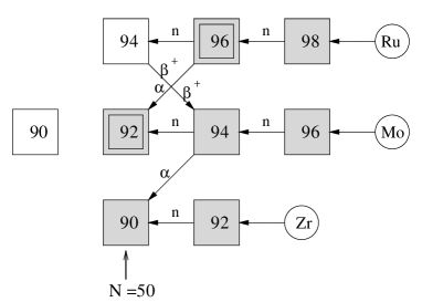
FIG. 1.: Nucleosynthesis path for ⁹²Mo and ⁹⁴Mo in the astrophysical $\gamma$-process. Stable nuclei are gray shaded. The nuclei ⁹²Mo and ⁹⁶Ru are marked; in this paper we determine an improved reaction rate for the ⁹⁶Ru($\gamma$,$\alpha$)⁹²Mo reaction. Note that the ($\gamma$,n) reactions stop at the magic neutron number $N=50$. The circles at the right end of the diagram mark several other stable nuclei.

FIG. 2.: Typical spectra at $E\approx 19$ MeV and $\vartheta_{\alpha}=25^{\circ}$ (upper diagram) and $E\approx 13$ MeV and $\vartheta_{\alpha}=145^{\circ}$ (lower diagram). The peak from elastic ⁹²Mo-$\alpha$ scattering is well separated from ¹²C-$\alpha$, ¹⁶O-$\alpha$ elastic scattering (upper) and from inelastic ⁹²Mo - $\alpha$ scattering (lower diagram).

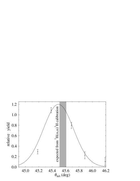
FIG. 3.: Relative yield of ¹²C recoil nuclei in coincidence with elastically scattered $\alpha$ particles. The shaded area shows the angle and the uncertainty which is expected from the calibration using the steep kinematics of ¹H($\alpha$,$\alpha$)¹H. The dotted line is a Gaussian fit to the experimental data points to guide the eye.

FIG. 4.: Experimental cross sections of ⁹²Mo($\alpha$,$\alpha$)⁹²Mo at $E_{\rm{c.m.}}\approx 13$, 16, and 19 MeV normalized to the Rutherford cross section. The lines are the result of optical model calculations (see table I).

FIG. 5.: Calculated cross sections of ⁹²Mo($\alpha$,$\alpha$)⁹²Mo at $E_{\rm{c.m.}}\approx 19$ MeV using five different parametrizations of the imaginary part of the potential. These five fits look very similar; however, fits 1, 4, and 5 have a significantly smaller $\chi^{2}$ (see Tables I and III).

FIG. 6.: Imaginary potentials of fits 1-5 of ⁹²Mo($\alpha$,$\alpha$)⁹²Mo at $E_{\rm{c.m.}}\approx 19$ MeV. The potential parameters are given in Tables I, II and III. Further details see text.

FIG. 7.: The variation of the strength parameter $\lambda$ of the real potential in a wide range shows the so-called “family problem”. Several minima in $\chi^{2}$ can be found. Further detail see text.

FIG. 8.: Real potentials for the different families 1-10 from Fig. 7. The potentials from families 2-5 which are well-defined as minima in $\chi^{2}$ (see Fig. 7) have the same depth $V(r)=-2.66$ MeV at the radius $r=8.52$ fm.

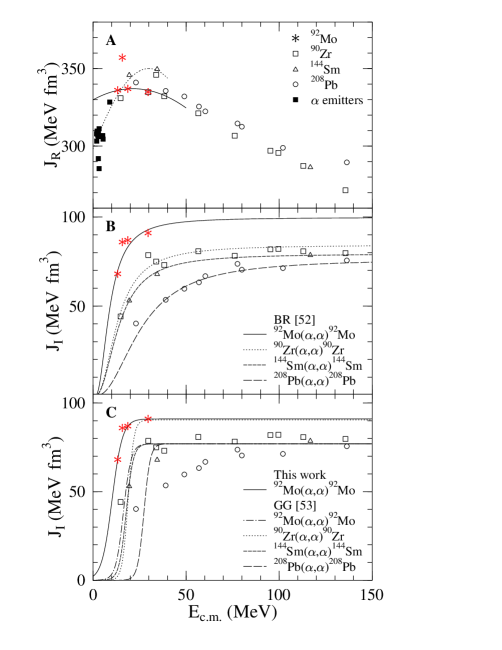
FIG. 9.: Volume integrals of the real (A, upper) and imaginary part (B and C, center and lower diagram) of the optical potential derived from ⁹²Mo($\alpha$,$\alpha$)⁹²Mo scattering. For comparison volume integrals derived from ⁹⁰Zr($\alpha$,$\alpha$)⁹⁰Zr, ¹⁴⁴Sm($\alpha$,$\alpha$)¹⁴⁴Sm, ²⁰⁸Pb($\alpha$,$\alpha$)²⁰⁸Pb scattering [31, 22], and from $\alpha$ emitters [32] were added. The lines in the upper diagram show Gaussian parametrizations of the new ⁹²Mo($\alpha$,$\alpha$)⁹²Mo data (full line) and from Ref. [32] (dotted line). The lines in the center diagram show the results of BR parametrizations [52] of the imaginary part. In the lower diagram the lines are the result of a Fermi-like parametrization from Grama and Goriely (GG) [53], using the parameters proposed by the authors, and the ones derived in this work (full line). Details see text.

FIG. 10.: Excitation function of ⁹²Mo($\alpha$,$\alpha$)⁹²Mo scattering at $\vartheta_{\rm{lab}}=170^{\circ}$ normalized to the Rutherford cross section. The experimental data are taken from Ref. [49]. The dotted (dashed, full) curves have been calculated from potentials which were adjusted to the 13 (16, 19) MeV angular distributions.

TABLE I.: Potential parameters of the imaginary part of the optical potential (combination of volume and surface WS parametrizations), derived from the angular distribution of ⁹²Mo($\alpha$,$\alpha$)⁹²Mo at $E=$13, 16 and 19 MeV, and its integral potential parameters $J$ and $r_{\rm{rms}}$ of their real and imaginary parts.

fit	$E$	$W_{V}~{}({\rm{MeV}})$	$R_{V}~{}({\rm{fm}})$	$a_{V}~{}({\rm{fm}})$		$W_{O}~{}({\rm{MeV}})$	$R_{O}~{}({\rm{fm}})$	$a_{O}~{}({\rm{fm}})$
1	19	-1.584	1.7667	0.2659		334.25	1.2605	0.2073
-	16	-9.558	1.668	0.248		308.20	1.348	0.099
-	13	-5.128	1.656	0.002		467.06	1.369	0.071
fit	$E$	$\lambda$	$w$	$J_{R}$	$r_{\rm{rms,R}}$	$J_{I}$	$r_{\rm{rms,I}}$	$\chi^{2}/F$
	(MeV)			$({\rm{MeVfm^{3}}})$	$({\rm{fm}})$	$({\rm{MeVfm^{3}}})$	$({\rm{fm}})$
1	19	1.257	1.003	337.2	4.991	86.2	5.806	2.15
-	16	1.346	0.9974	357.8	4.976	85.9	5.992	4.84
-	13	1.352	0.9758	336.7	4.869	67.3	6.043	1.26

TABLE II.: Potential parameters of the imaginary part of the optical potential (volume and surface WS parametrization), derived from the angular distribution of ⁹²Mo($\alpha$,$\alpha$)⁹²Mo at $E=$19 MeV, and its integral potential parameters $J$ and $r_{\rm{rms}}$ of their real and imaginary parts.

fit	$W_{V}~{}({\rm{MeV}})$	$R_{V}~{}({\rm{fm}})$	$a_{V}~{}({\rm{fm}})$		$W_{O}~{}({\rm{MeV}})$	$R_{O}~{}({\rm{fm}})$	$a_{O}~{}({\rm{fm}})$
2	-10.806	1.7116	0.3601
3					121.76	1.4947	0.4206
fit	$\lambda$	$w$	$J_{R}$	$r_{\rm{rms,R}}$	$J_{I}$	$r_{\rm{rms,I}}$	$\chi^{2}/F$
No.			$({\rm{MeVfm^{3}}})$	$({\rm{fm}})$	$({\rm{MeVfm^{3}}})$	$({\rm{fm}})$
2	1.237	1.010	341.1	5.037	57.9	6.131	3.67
3	1.188	1.021	338.9	5.095	80.6	6.957	4.28

TABLE III.: Potential parameters of the imaginary part of the optical potential (FB para- metrization), derived from the angular distribution of ⁹²Mo($\alpha$,$\alpha$)⁹²Mo at $E=$19 MeV, and its integral potential parameters $J$ and $r_{\rm{rms}}$ of their real and imaginary parts.

fit	$R_{\rm{FB}}~{}({\rm{fm}})$	$a_{1}$	$a_{2}$	$a_{3}$	$a_{4}$	$a_{5}$	$a_{6}$	$a_{7}$
4	12.8	154.94	-311.98	839.41	-325.97	880.41	-	-
5	12.0	167.94	-329.11	1103.43	-592.10	1666.61	-346.79	1118.06
fit	$\lambda$	$w$		$J_{R}$	$r_{\rm{rms,R}}$	$J_{I}$	$r_{\rm{rms,I}}$	$\chi^{2}/F$
No.				$({\rm{MeVfm^{3}}})$	$({\rm{fm}})$	$({\rm{MeVfm^{3}}})$	$({\rm{fm}})$
4	1.272	0.998		338.8	4.979	68.2	4.524	2.23
5	1.287	0.991		336.0	4.947	53.9	4.319	2.14

TABLE IV.: Potential parameters of the imaginary part of the optical potential (combination of volume and surface WS parametrizations), derived from the angular distribution of ⁹²Mo($\alpha$,$\alpha$)⁹²Mo from Refs. [47] and [48], and its integral potential parameters $J$ and $r_{\rm{rms}}$ of their real and imaginary parts.

Ref.	$W_{V}~{}({\rm{MeV}})$	$R_{V}~{}({\rm{fm}})$	$a_{V}~{}({\rm{fm}})$	$W_{O}~{}({\rm{MeV}})$	$R_{O}~{}({\rm{fm}})$	$a_{O}~{}({\rm{fm}})$
[47]	-4.91	1.78	0.40	183.13	1.13	0.36
[48]	-3.51	1.72	0.95	337.06	1.26	0.23
Ref.	$\lambda$	$w$	$J_{R}$	$r_{\rm{rms,R}}$	$J_{I}$	$r_{\rm{rms,I}}$
No.			$({\rm{MeVfm^{3}}})$	$({\rm{fm}})$	$({\rm{MeVfm^{3}}})$	$({\rm{fm}})$
[47]	1.19	1.022	334.76	5.098	90.95	5.704
[48]	1.15	1.014	315.49	5.056	107.91	6.014

TABLE V.: Extrapolated values of the potential paramters of the imaginary part of the optical potential at the astrophysically relevant energies $E_{0}=5.8$ MeV ($T_{9}=2.0$) and $E_{0}=7.6$ MeV ($T_{9}=3.0$), and its integral potential parameters $J$ and $r_{\rm{rms}}$ of their real and imaginary parts.

$E$	$W_{V}~{}({\rm{MeV}})$	$R_{V}~{}({\rm{fm}})$	$a_{V}~{}({\rm{fm}})$		$W_{O}~{}({\rm{MeV}})$	$R_{O}~{}({\rm{fm}})$	$a_{O}~{}({\rm{fm}})$
7.6	-1.466	1.717	0.268		36.86	1.295	0.419
5.8	-1.091	1.720	0.270		27.44	1.297	0.420
$E$	$\lambda$	$w$	$J_{R}$	$r_{\rm{rms,R}}$	$J_{I}$	$r_{\rm{rms,I}}$	$\chi^{2}/F$
(MeV)			$({\rm{MeVfm^{3}}})$	$({\rm{fm}})$	$({\rm{MeVfm^{3}}})$	$({\rm{fm}})$
7.6	1.219	1.000	327.1	4.991	26.2	6.085	-
5.8	1.209	1.000	324.3	4.991	19.6	6.095	-

TABLE VI.: Parameters of the BR and Fermi parametrizations of the imaginary volume integral $J_{I}$ for ⁹²Mo($\alpha$,$\alpha$)⁹²Mo.

parametrization	saturation value	rise parameter	other parameters
BR	$J_{0}=99.8$ MeV fm3	$\Delta=7.68$ MeV	$E_{0}=1.51$ MeV
Fermi	$J_{0}=91.0$ MeV fm3	$a^{\ast}=2.78$ MeV	$E^{\ast}=10.24$ MeV

TABLE VII.: Most effective energies $E_{0}$ for the ⁹²Mo($\alpha$,$\gamma$)⁹⁶Ru and the ⁹⁶Ru($\gamma$,$\alpha$)⁹²Mo reactions.

$T_{9}$	$E_{0}(\alpha,\gamma)$	$E_{0}(\gamma,\alpha)$
2.0	5.81	7.51
2.5	6.75	8.44
3.0	7.62	9.31

TABLE VIII.: Ratio $\xi=r_{x}/r_{0}$ of the astrophysical reaction rates $r_{x}$ obtained with different imaginary potentials to a standard rate $r_{0}$ [15, 17].

$T_{9}$	GGa	ESWb	A c ($T_{9}=2$)	B d ($T_{9}=3$)	AB e
2.0	0.014	0.121	0.453	0.497	0.503
3.0	0.012	0.140	0.546	0.579	0.585

TABLE IX.: Variation of the imaginary part of the potential derived for $T_{9}=2.0$. Rate ratios are shown in respect to the rate obtained with the parameters for $E=5.8$ MeV ($J_{I}=19.6$ MeV fm³, 70% surface contribution) from Tab. V.

	Variation of $J_{I}$			Surface Contribution
T	$J_{I}=$	$J_{I}=$		$J_{I}=19.6$ MeV fm3
109 K	15.4 MeV fm3	23.9 MeV fm3		90%	80%	60%	50%
0.5	0.942	1.077		0.952	0.976	1.019	1.043
1.0	0.949	1.070		0.949	0.975	1.032	1.057
1.5	0.913	1.078		0.937	0.968	1.029	1.057
2.0	0.902	1.077		0.937	0.969	1.029	1.056
2.5	0.918	1.062		0.945	0.974	1.026	1.049
3.0	0.945	1.050		0.958	0.981	1.020	1.040
3.5	0.968	1.027		0.966	0.984	1.016	1.030
4.0	0.991	1.013		0.977	0.988	1.010	1.021
4.5	1.007	1.001		0.983	0.992	1.006	1.014
5.0	1.019	0.995		0.989	0.995	1.005	1.009
6.0	1.028	0.991		1.000	1.000	1.000	1.009
7.0	1.031	0.985		0.999	0.999	1.000	1.000
8.0	1.026	0.987		1.000	1.000	1.000	0.996
9.0	1.020	0.990		1.004	1.002	0.998	0.996
10.0	1.011	0.994		1.005	1.002	0.998	0.994