Automatic variability analysis of bulge stars in OGLE II image subtraction database

Abstract

We present results of star variability analysis in OGLE II first bulge field. Photometric database was derived by means of image subtraction method (Woźniak 2000) and contains 4597 objects pre-classified as variables. We analyzed all the light curves in order to find periodic variables, non periodic but all-time variables and stars showing episodic changes in their brightness, e.g. gravitational lenses. Variability of 3969 stars was confirmed, among them we detected 12 lensing event candidates whose light curves are shown. We found 762 periodic variables. Algorithmic methods let us identify 71 RR Lyrae and 110 W UMa stars. Almost all luminous red giants are found to be variable. Most of red clump giants are not variable. Classification of all 4597 objects is presented online.

Warsaw University Observatory, Al. Ujazdowskie 4, 00-478 Warszawa, Poland

mizerski, bejger@astrouw.edu.pl

1 Introduction

The observational data were obtained with Warsaw 1.3m telescope located at Las Campanas Observatory of the Carnegie Institution of Washington, and instruments ("Zero generation" single chip, camera SITe 2048$\times$2048 thin chip) dedicated to the second phase of the Optical Gravitational Lensing Experiment - OGLE II. In the years 1997 - 1999 about 200 observations were made, mainly in drift scan mode in the I photometric band. Single image is 8192x2048 pixels (55’x14’) in size - we refer to Udalski, Kubiak & Szymański (1997) for the technical details of instruments and the telescope.

The photometric data based on the algorithm of Alard & Lupton (1998) and Alard (2000) and derived by P.R.Woźniak (Woźniak 2000) can be downloaded from http://astro.princeton.edu/~wozniak/dia.

The article is arranged in the following order: Section 2 describes our method of rejecting spurious variables. In section 3 we describe the method and results of periodic variability analysis. Afterwards, in section 4, search for specific variability types - RR Lyrae and W UMa stars - is reviewed. Section 5 is dedicated to non periodic variables. We discuss methods of detecting such stars - as an example, simply statistical algorithms let us identify 12 gravitational lensing events, in one case with lensed star being irregular variable itself. At the end of the article, in section 6, we present color-magnitude diagram for detected variables and demonstrate the luminosity function of the field.

2 Spurious variables

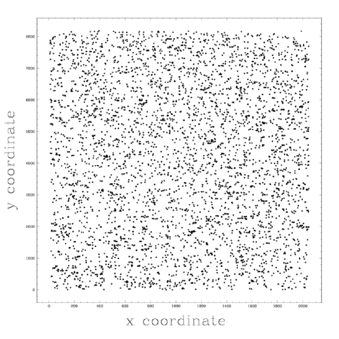
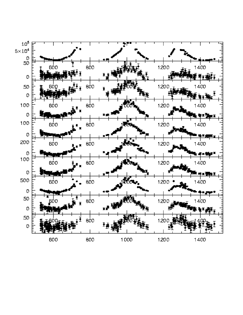
Some objects pre-classified as variables may not in fact be truly variable. Apparent and especially temporary changes in brightness can be caused by instrumental defects or by the method itself. If such stars tend to gather in groups in the imaged field their variability is very improbable. In Fig. 1 we demonstrate locations of all stars on the reference image coordinate plane. As we can see correlations between positions of some objects are noticeable. By investigating all dense regions we found groups of artificial variables. In the case illustrated on Fig. 2 one very bright variable influenced nine of its faint constant neighbors and produced nine spurious variable stars. To detect all such cases we performed following procedure for every variable star: within the 100 pixel radius we searched for stars whose light curves were correlated with the light curve of the star. If the correlation coefficient was greater than 0.75 the stars were considered correlated and thus only the brightest one could be regarded as a real variable. In Fig. 3 we show histogram of distances between luminous variable stars and spurious variables produced by them. Choosing the radius of 100 pixels may result in finding few stars correlated by chance but ensures that most of the spurious variables are rejected.

As a result we found 254 groups of correlated light curves and 363 stars were classified as spurious variables. This problem concerns objects of all possible variability types. Setting the correlation coefficient limit lower than 0.75 excludes real variables.

Independently, stars exhibiting high proper motions were also taken into account. Those stars produce pairs of anti-correlated light curves. There are 98 such pairs. For more details on stars with high proper motions we refer to Eyer & Woźniak (2001).

This improved classification decreased the number of variable candidates from 4597 to 3969 objects.

3 Periodic variables. Criteria of acceptance

The OGLE II database of the first bulge field bul_sc1 ($\alpha_{2000}=18\mathrm{h}\,02\mathrm{m}\,32.5\mathrm{s},\>\beta_{2000}=-29^{\mathrm{o}}57^{\prime}41^{\prime\prime},\>l=1.08^{\mathrm{o}},\>b=-3,62^{\mathrm{o}})$ consists of about 200 frames from three observational seasons. The time span $\Delta t$ is $\sim$ 1000 days. Two periodic signals with frequencies that differ by $\Delta\nu$ will after $\Delta t$ end up having phase difference $\Delta\varphi$ = $2\pi\Delta\nu\cdot\Delta t$. We demand $\Delta\varphi$ $\sim$ $10^{-2}$ which gives $\Delta\nu$ $\sim$ $10^{-5}.$ With such a frequency step periodogram generation takes a lot of CPU time if we search for short periods, i.e. high frequencies. The only way to avoid this is to have a shorter time span $\Delta t$. We decided to search for short periodic variables using only the data points from the first season. There are about 100 such points and $\Delta t$ is only 200 days. This allows setting a greater frequency step in periodogram generator, namely $10^{-4}$ [$\mathrm{d}^{-1}$]. Time span of about 200 days is robust enough for detecting variables with periods shorter than 50 days - the most CPU consuming part. Variables with periods longer than 50 days were searched for on the whole data set with frequency step equal to $10^{-5}$ [$\mathrm{d}^{-1}$].

We used Analysis of Variance algorithm (Schwarzenberg-Czerny 1989) to obtain probable periods for every star. If such periods were found next step was to check if any of them is physical. Using the usual $\chi^{2}$ minimization, for each period a Fourier series was fitted to the data points. Number of harmonics was set to six which is good enough to approximate most of the light curve shapes. The purpose was not to refine the period but to find the coefficients of the fit, that is amplitudes of all harmonic terms. The formula for $\chi^{2}$ is given below:

$$\chi^{2}=\frac{1}{n-b}\cdot\sum^{n}_{i=1}\frac{1}{\sigma^{2}_{i}}\cdot\left(f_{i}-\sum^{m}_{j=0}(A_{j}\cdot\sin(j\omega t_{i})+B_{j}\cdot\cos(j\omega t_{i}))\right)^{2}$$ (1)

where $n$ is the number of data points, $m$ is equal to the number of harmonics, $b$ is equal to the number of degrees of freedom used for fit calculation; $b=2m+1$, $f_{i}$ is the value of flux on the i-th frame, $t_{i}$ represents time of the i-th observation, $\sigma_{i}$ is the corresponding flux error and $A_{j}$ and $B_{j}$ are the harmonic terms amplitudes. Once an analytical approximation of the curve was found it was possible to determine the quality of the fit. Our parameter is defined as follows:

$$\rho=\frac{\frac{1}{n-b}\cdot\sum^{n}_{i=1}\left(f_{i}-\sum^{m}_{j=0}(A_{j}\cdot\sin(j\omega t_{i})+B_{j}\cdot\cos(j\omega t_{i}))\right)^{2}}{\frac{1}{n-1}\cdot\sum_{i=1}^{n}\left(f_{i}-\frac{1}{n}\cdot\sum^{n}_{j=1}f_{j}\right)^{2}}$$ (2)

Parameter $\rho$ measures dispersion from the fit and, contrary to $\chi^{2}$, does not prefer low amplitude objects. For two sinusoidal curves with the same period but different amplitudes, $\chi^{2}$ is significantly different, while $\rho$ stays very much the same. For true periods it is mostly on the order of $10^{-3}$ - $10^{-1}$ while spurious periods give relatively much higher values of $\rho$.

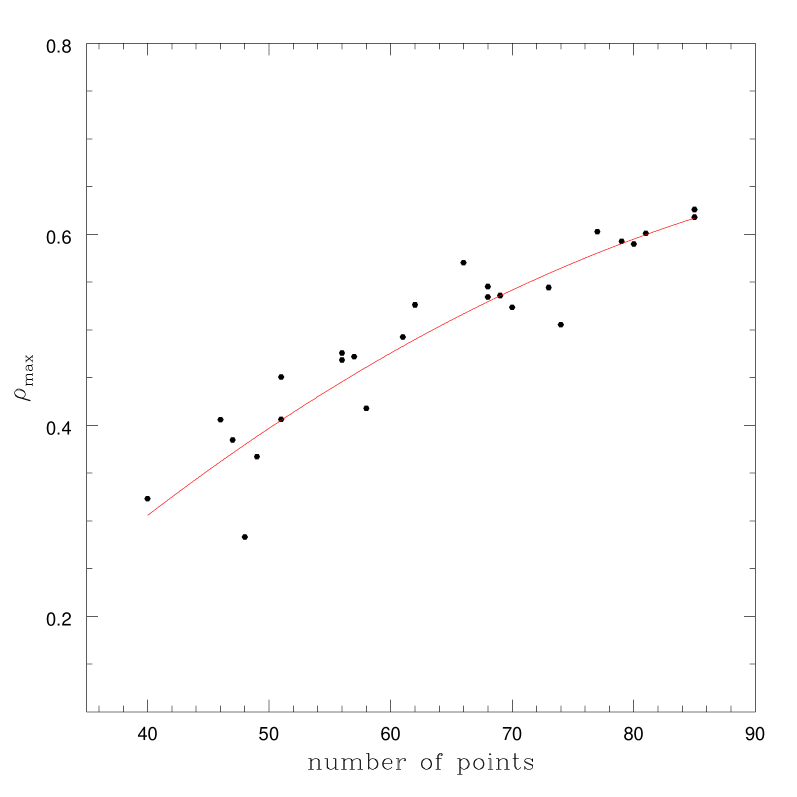
Next thing to do was to find $\rho$_max - the upper limit for the value of $\rho$ as the criterion of acceptance. For every star a list with possible periods and corresponding $\rho$’s was produced. We then sought the smallest $\rho$ on the list. The star was considered periodic variable, when the value of $\rho$ was smaller than the limit of acceptance i.e. the value of $\rho_{\mathrm{max}}$. One should not expect one universal value for $\rho_{\mathrm{max}}$: note, that it is easier to get a low $\rho$ by chance when number of data points is smaller. That’s why $\rho_{\mathrm{max}}$ should rather be a monotonically increasing function of $n$. For the first season values of $n$ are between 40 and 90. We chose 22 stars with different number of data points in this range.

For each of those 22 stars we generated 100 different artificial light curves by shuffling their data points with corresponding errors. In the next step we obtained suspected periods for all the generated curves and for each we chose the period with the smallest $\rho$. As the result we got 22 lists with 100 smallest $\rho$ each. For every list, which as we remember corresponds to a different n, we chose $\rho_{\mathrm{max}}$ so that only 2 out of 100 artificial stars would a have smaller $\rho$. We arbitrarily defined $\rho_{\mathrm{max}}$ as the mean value of the second and the third smallest $\rho$. Finally we approximated the relation between $\rho_{\mathrm{max}}$ and $n$ with parabola using least squares. The result is shown in Fig. 4. Having an analytical function $\rho_{\mathrm{max}}(n)$, we were able to determine $\rho_{\mathrm{max}}$ for any $n$. Our prescription implies that we allow about 2 per cent spurious stars into periodic variable class. The goal is not to miss very noisy periodic stars.

The last step of verification was the same $\rho$ test but on the other two remaining observational seasons. The stars that had passed all these tests were considered periodic variables. This procedure in the case of multi periodic behavior would produce only one period - the better fitted one. For example first overtone for RR Lyrae type d stars would be considered as the physical period. It is not of a great importance since the star would still be classified as a periodic variable.

3.1 Results

Using these techniques we found 487 periodic variables with periods shorter than 50 days. The last step of verification - $\rho$ test on the other remaining observational seasons turned out to be very important. Periodic variability of only 487 of 1157 stars considered periodic variable on the first season was confirmed. There are 265 stars with $P\leq 1[d]$, 112 stars with $1[d]<P\leq 10[d]$ and 110 stars with $10[d]<P\leq 50[d]$ among periodic variables detected in this field.

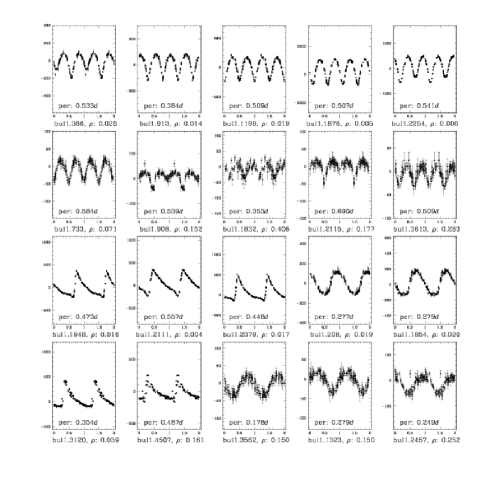
Those are pulsating, eclipsing and miscellaneous type stars. Miscellaneous class contains chromospherically active giants, sub giants and ellipsoidal variables as well as all uncertain cases. Most of the eclipsing binaries are Algol and W UMa type variables. Pulsators are mainly RR Lyrae and High Amplitude $\delta$ Scuti (HADS) stars. Some examples are presented in Fig. 5.

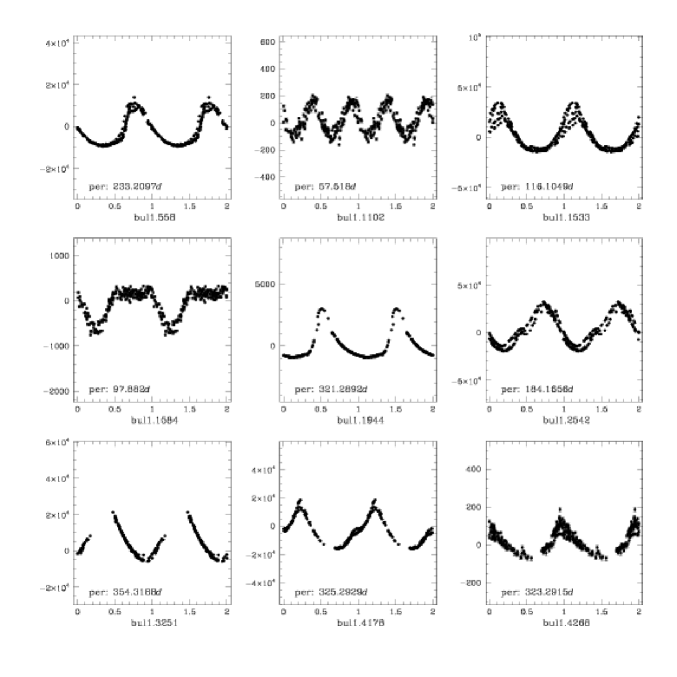
We also sought variables with periods longer than 50 days - 275 objects exhibit strictly or more or less quasi periodic behavior. Examples are shown in Fig. 6.

4 Algorithmic methods for identification of common variability types

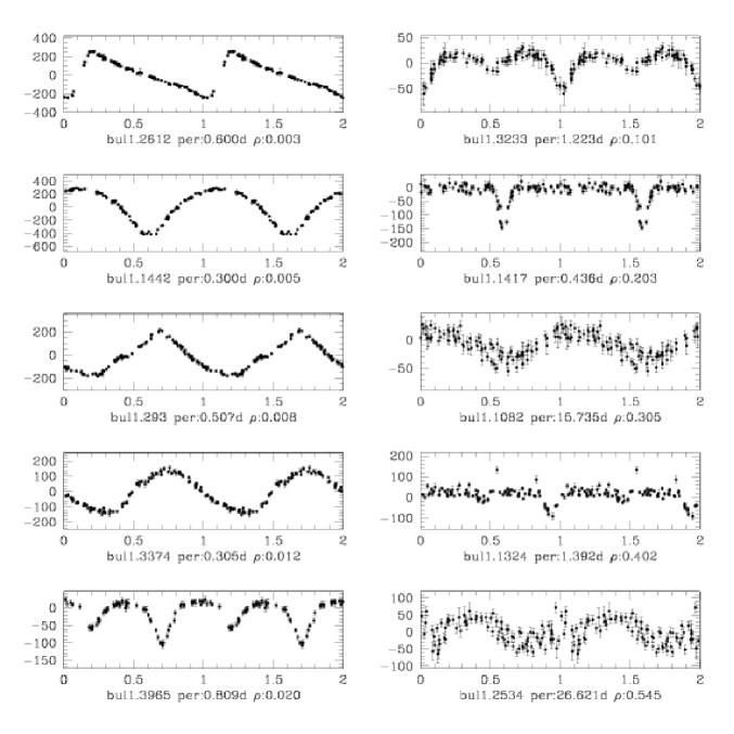
After we had found periodic variables, we sought specific types of variability: RR Lyrae and W UMa. There are well known methods of identifying these types by means of Fourier series coefficients. For RR Lyrae we refer to Alard (1996) and for W UMa to Ruciński (1993). Our code, based on those methods, but with slightly modified parameters, detected 47 RRab, 24 RRc and 110 W UMa stars. Apart from RR Lyrae our algorithm returned also 11 possible HADS stars. That is because separating HADS and RRc is not always simple. Their light curve shapes are sometimes similar to those of RR Lyrae type c stars. The main goal of the method was to detect the types of variability by “looking” at the curve shape only. In case of HADS stars we needed some additional parameters (like luminosity) to make a choice. In Fig. 7 we present sample light curves with different dispersions. In the last row three last stars are HADS stars candidates. The judgment is very problematic: their amplitudes are much smaller than those of typical RR Lyrae type c, their Fourier coefficients however are more RRc alike and the periods are longer than 0.2 d. Thus, we would like to leave the ultimate judgment to the reader.

5 Non periodic variable stars

5.1 Variance analysis

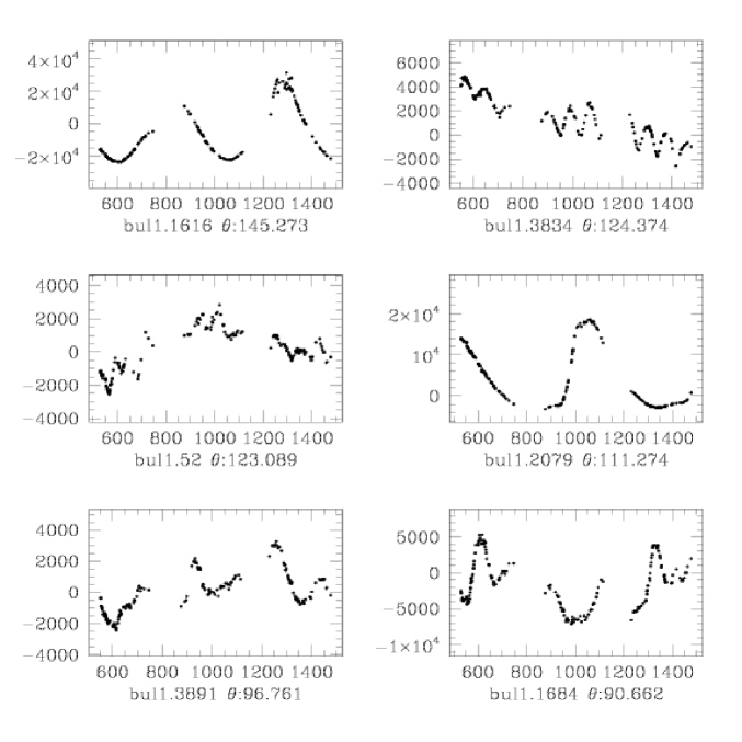
We used Analysis of Variance (AoV) in very much the same manner as Brandt (1970) described. Whole data set was divided into packets, 10 observations each, and mean value, as well as variance, was computed in every packet. Then we calculated the variance of those mean values and mean packet variance. Their ratio $\theta$ is an officious variability indicator since it tests mean values equality hypothesis. As one can see in Fig. 8, this algorithm works well for irregular behavior detection. A constant star has $\theta\sim 1$ while for most of the microlensing events found in this field $\theta$$\in[10,\,100]$. 1341 stars had their $\theta>10$, and this value seems to be a reasonable cut-off. Weak lenses failed this test, but were detected by other means - as described in section 5.3.

5.2 Hunting noisy variables

Some stars exhibit a noisy behavior. To distinguish between a weak variable star and photon noise, and to find all the cases where subsequent data points are correlated, we developed the following test. Each data point was regarded as positive/negative if it was greater/smaller than the weighted average of the whole curve. Such treatment produces a time series of points, marked as 1 or -1 respectively. Along with time there are positive-negative state transitions, i.e. sign changes, which have a binomial distribution. In the case of photon noise this distribution is symmetric, since any point has equal probabilities of being smaller or greater than the average $N/2$, where $N$ is the number of possible sign changes. For each light curve we compared its own distribution of sign changes with the binomial distribution i.e. we calculated the probability

$$P^{K}_{N}(\left|N/2-k\right|\geq\left|N/2-K\right|)$$ (3)

where $k$ is the number of sign changes in $N$ possibilities, and $K$ equals the observed number of sign changes. We classified as variables all the light curves with $P^{K}_{N}\leq P(\left|N/2-k\right|\geq 3\sigma)$, with binomial distribution standard deviation $\sigma$$=\sqrt{N}/2$. There are 3447 such objects in the database, which leads to conclusion, that 522 stars were classified as non-variables by this test. Fig. 9 shows the histogram of computed probabilities against the logarithm of the number of stars. Most of the rejected stars are stars with short time scales of variability. One day sampling of the OGLE data can randomize flux distribution as far as this test is considered. It does not affect long time scale variables since their light curves are sampled with frequencies sufficient to reveal night to night correlations. The short time scale variables, such as RR Lyrae or W UMa stars were classified as variables by other means.

5.3 Search for episodic variability

Episodic variables such as gravitational lenses or long period eclipsing binaries are easy to found using very simple statistical methods (of course, periodic behavior was mainly detected by the use of methods described in section 3). We rejected 10% points with greatest absolute values of flux to calculate the average value and dispersion. After those quantities were found we analyzed each point‘s deviation from the average value and counted separately all those cases where the absolute value of deviation was

1) greater than $3\sigma$ but smaller than $6\sigma$ (number of these points: $n_{3}$)

2) greater than $6\sigma$ but smaller than $9\sigma$ ($n_{6}$)

3) greater than $9\sigma$ ($n_{9}$)

The star was considered episodic variable if it satisfied at least one of these arbitrary chosen criteria:

1) n₃ $\geq$ 6

2) n₆ $\geq$ 3

3) n₉ $\geq$ 3

4) n₉ $\geq$ 2 and n₆ $\geq$ 2

5) n₉ $\geq$ 1 and n₃ $\geq$ 3

6) n₆ $\geq$ 1 and n₃ $\geq$ 3

We found 1710 such stars, some of them being not really episodic, but undoubtedly variable, e.g. Mira-type stars. We also calculated the value of a parameter defined as follows:

$$p=\frac{1}{3\cdot n_{3}+6\cdot n_{6}+9\cdot n_{9}}$$ (4)

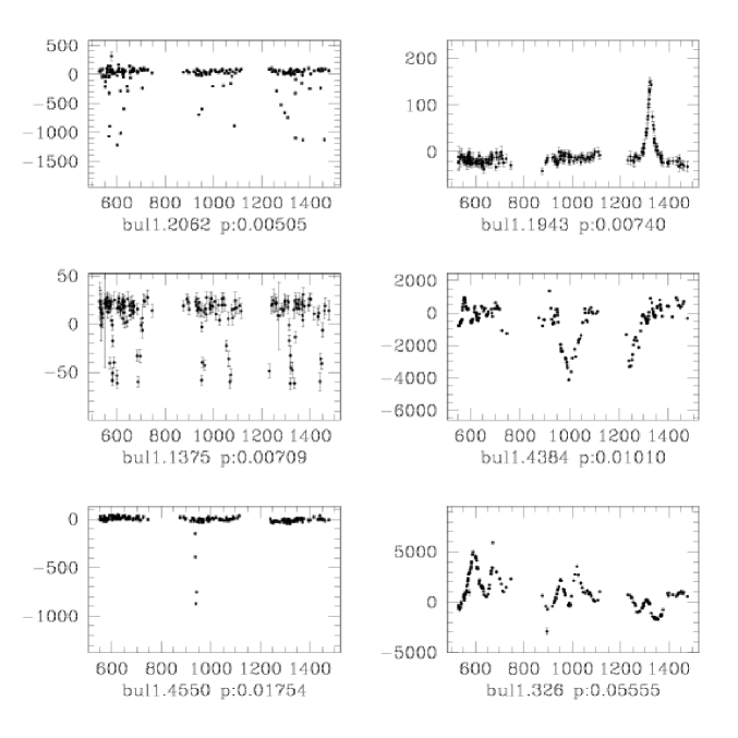
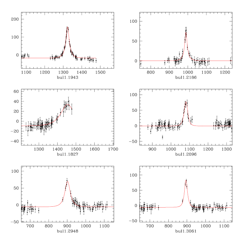
This parameter is selective: it prefers points with greater deviations. Among the stars with smallest values of p is a gravitational lens bul_sc1.1943 which is shown on Fig. 10 along with other examples. This strong lensing event had not been detected previously with the use of DoPhot. In section 6 we give a possible explanation for this.

5.4 Results. Gravitational lenses

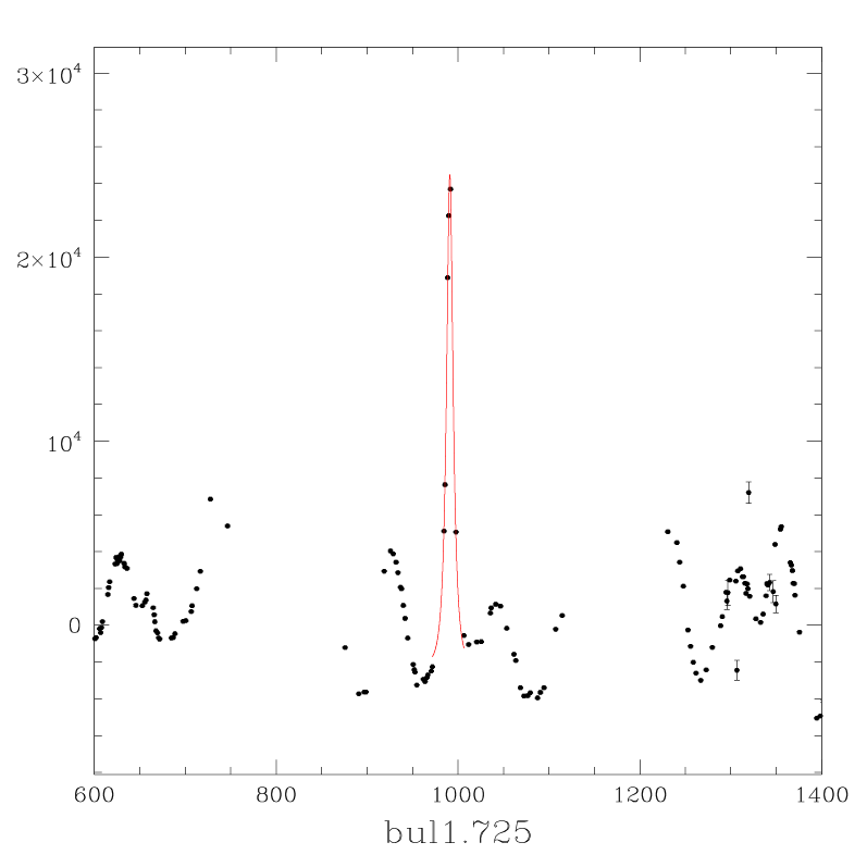
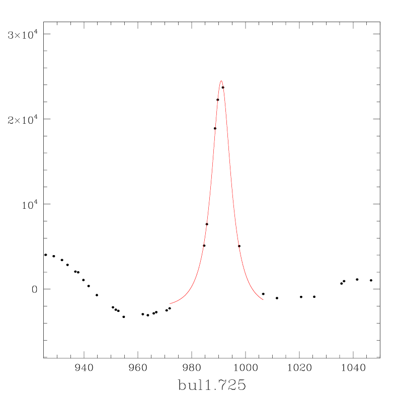
About 3950 stars passed at least one of the complementary tests described above. In this number we identified 12 gravitational lens candidates. Woźniak et al. (2001) reports 2 lenses in this field, that is bul_sc1.1943 and bul_sc1.2186. All the others with exception for bul_sc1.3061 and bul_sc1.725 are in their “transient” catalogue. This results from stronger criteria used by those authors. In table 1 we present theoretical models fitted to the data. Purely mathematical approach to the fitting procedure may result in unphysical values of some parameters because of degeneracy of the model curve. In the case of bul_sc1.725, presented in Fig. 11, lensed star is variable itself, thus there is no point in calculating a theoretical fit to the whole curve. However, we show a fit to the data around the point of maximum magnification.

star	1943	2186	1827	2096	2948	3061	2411	2724	3844	3087	3327
$\chi^{2}$	1.03	1.27	1.03	1.49	1.04	1.16	1.30	1.51	1.33	1.27	1.07
$\mathrm{t}_{\mathrm{max}}$ [d]	1323.48	989.86	1454.61	1080.95	901.76	894.31	602.83	989.97	625.92	967.72	601.70
$\mathrm{t}_{0}$ [d]	26.13	25.88	39.15	19.14	31.13	15.27	10.92	1071.71	8.32	2.51	148.64
$u_{0}$	1.29	0.23	1.29	0.51	0.46	0.56	0.15	0.0014	0.50	1.69	0.11

Table 1: $\chi^{2}$ values and computed parameters for eleven gravitational lensing event candidates

The remaining 11 candidates also seem realistic since in each case scatter around the theoretical fit, described by $\chi^{2}$ per degree of freedom, is $\sim$ 1 (see table 1 for details). However, $\chi^{2}$ values given in table 1 were not obtained using nominal errors provided by the photometric data pipeline of Woźniak (2000). In some cases some error rescaling was needed prior to the calculation of the fit. The reason for this is that image subtraction method has minor problems with data error overestimation. Without rescaling 10 curves had their $\chi^{2}$ significantly smaller than 1. Error scaling factor, determined for each curve separately, was defined as the ratio of flux dispersion to average error. To compute the scaling factor we used only data points from the baseline of the light curve. Baseline was defined as 75 percent of all data points with smallest values of flux.

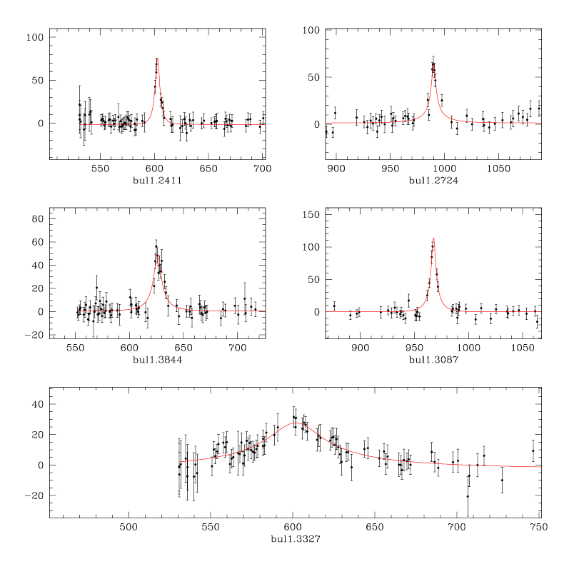
Light curves of remaining 11 lenses are presented at Fig. 12 and Fig. 13. Though bul_sc1.2948 and bul_sc1.3061 may look similar, they are separated on the reference frame by 347 pixels in x-coordinate and by 136 pixels in y-coordinate. This gives centroids distance about 372 pixels which is quite large comparing to the size of the image and makes a hypothesis of them being related to each other rather unlikely.

6 Luminosity function and color-magnitude diagram

We DoPhoted the reference frame in order to match star positions from our variable star database with those found by DoPhot (for the detailed process of making the reference image see Woźniak 2000). For every star in our database we sought the closest DoPhot star within a 3 pixel radius. Due to the blending effect some of the variable stars from the database were not detected by DoPhot. Almost 180 stars were not matched. Some others were identified with the same DoPhot star. This problem concerns about 260 objects (there are 130 pairs of identically matched stars). Most of them are stars with large proper motions, for details see Eyer & Woźniak (2001).

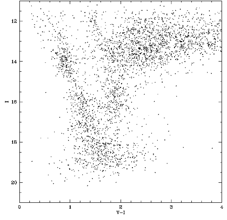
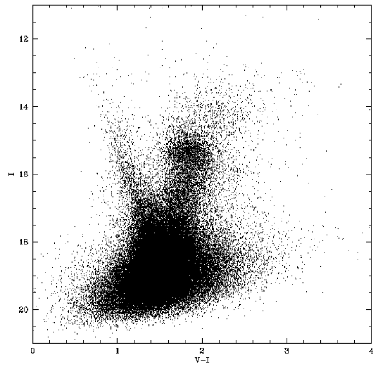
In Fig. 14 we show luminosity function for specific variability classes. We also present the same function for the whole field, i.e. all stars found by DoPhot. As one can see Fig. 14 suggests that almost all bright stars are variable. Color-magnitude dependence for the field obtained by OGLE is shown in Fig. 15 in the lower panel, in which all the variables were subtracted and only one per every 7 stars was plotted for clarity. The upper panel contains the same diagram for variable stars. Most of the brightest stars are red giants. Group of Red Clump variables is dominated by stars with spots.

Our analysis confirms variability of most of the bright objects but in some cases apparent variability may be due to the presence of saturated data points or problems with the PSF. We rejected only obviously spurious variables. Also notice that there are some non periodic variable stars with $\mathrm{I}_{\mathrm{mag}}>20$. Some of them, but certainly not all, may in fact be spurious variables like those described in section 2 but with correlation coefficients smaller than 0.75. Presence of some others may be due to different kinds of instrumental defects. Nevertheless there are some real, weak, irregular variables with $\mathrm{I}_{\mathrm{mag}}>20$ of rather unknown nature. The use of difference image analysis results in higher number of specific variables found, e.g. gravitational lenses described in section 5.4. For example, during our search for episodic variables we found a strong gravitational lens, bul_sc1.1943, which is located near another, brighter star. This lens had not been detected previously with the use of DoPhot by Udalski et al. (2000). It presumably merged with its bright neighbor‘s PSF wings and therefore was not identified. In Fig. 16 we demonstrate variability scale for variable stars of all kinds - note the position of gravitational lensing candidates. They are located along the line of detection limit. Objects forming very dense clump around 13 mag cover a wide range from blue to red stars in Fig. 15. The fluxes were converted to magnitudes as Woźniak (2000) described.

7 Summary and conclusions

The database, derived by means of image subtraction method, contains only 4597 objects that were suspected of variability during the database generation process. This value is 100 times smaller than the number of stars found on the reference image by DoPhot. We classified 3969 of those 4597 stars, that is about 85%, as variables using the data pipeline described above. Our methods are complementary and so a given star can pass more than one variability test. For example some Mira type pulsators were not only found as periodic but also as episodic variables as well. This was taken into account at the very end, after all the tests had been performed. Final results of classification can be found at: ftp://ftp.astrouw.edu.pl/pub/mizerski/bul1.table in the form of the classification table presented below:

 

#     ra:             dec:          <Imag>: std_dev:    V-I:    per:  flag:

1     18:02:01.07     -30:25:27.7     16.034   0.001214    -99.999  50.951 long

2     18:02:01.55     -30:25:07.2     14.014   0.000046    -99.999 -99.999 var

3     18:02:05.00     -30:25:25.1     12.282   0.003312      2.206 -99.999 e

4     18:02:06.53     -30:25:02.7     12.279   0.005765      4.338 -99.999 var

5     18:02:07.20     -30:25:07.3     15.323   0.000792      1.927 -99.999 var

6     18:02:08.42     -30:25:42.9     13.774   0.000077      3.086 -99.999 var

7     18:02:09.53     -30:25:15.1     13.029   0.000617      4.436 -99.999 var

8     18:02:13.42     -30:25:52.0     18.649   0.312950      1.842 -99.999 e

9     18:02:01.68     -30:25:35.6     18.671   0.040266    -99.999 -99.999 var

10     18:02:03.95     -30:25:27.3     14.253   0.000031      2.395 -99.999 var

11     18:02:04.24     -30:25:52.8     13.883   0.000041      2.289 -99.999 var

12     18:02:07.07     -30:25:16.3     17.639   0.021581      1.492   0.249 wuma

Details can be found in a readme.txt file on the web.

Our methods let us detect 487 short periodic variables, with 71 RR Lyrae, 110 W UMa stars among them and 275 long periodic variables. We also detected 12 gravitational lenses candidates. The last result is very promising since with the use of DoPhot only one lens, bul_sc1.2186, had been previously found in this field (Udalski et al. 2000). This is due to higher quality photometry and different search methods: bul_sc1.725, which is possibly a lensing event of a variable star, could not have been detected using constant stars catalogue. On the other hand, the strongest lens bul_sc1.1943 was not identified by DoPhot as it presumably merged with another star PSF wings. Woźniak et al. (2001) detected 2 lenses in this field: bul_sc1.1943 and bul_sc1.2186. Our others lenses, with exception for bul_sc1.3061 and bul_sc1.725, are in their “transient” catalogue.

We conclude that image subtraction method is much more efficient in massive variability searches.

Acknowledgments

First of all we would like to thank Dr. Bohdan Paczyński for all the advice and helpful discussions and Dr. Wojciech Dziembowski, who carefully read the script and gave us many valuable suggestions. We also thank Przemek Woźniak who created the database and OGLE team at Warsaw for giving us access to their data.

This work was partly supported by the NSF grant AST-9820314 to Bohdan Paczyński.

References

Alard, C., 1996, Astrophys. J., 458, L17

Alard, C., 2000, A&AS, 144, 363

Alard, C., Lupton, R. H., 1998, Astrophys. J., 503, 325

Brandt, S., 1970, Statistical and Computational Methods in Data Analysis, North-Holland Publishing Company

Eyer, L., Woźniak, P., 2001, astro-ph/0102027

Ruciński, S. M., 1993, PASP, 105, 1433

Schechter, P., Mateo, M., & Saha, A., 1995, PASP, 105, 1342

Schwarzenberg - Czerny, A., 1989, Mon. Not. R. astr. Soc., 241, 153

Udalski, A., Kubiak, M., & Szymański, M., 1997, Acta Astron., 47, 319

Udalski, A., Żebruń, K., Szymański, M., Kubiak, M., Pietrzyński, G., Soszyński, I., & Woźniak, P., 2000, Acta Astron., 50, 1

Woźniak, P., 2000, Acta Astron., 50, 421

Woźniak, P., Udalski, A., Szymański, M., Kubiak, M., Pietrzyński, G., Soszyński, I., Żebruń, K., 2001, arXiv:astro-ph/0106474v1

Figure 1: Coordinate plane of the reference image. Note the groups of stars - in many cases a bright star influences its faint neighbors and produces spurious variable stars.

Figure 2: Real variable (top window) and nine fake variables located in its vicinity.

Figure 3: Histogram of distances between correlated genuine bright variables and spurious variables.

Figure 4: Dependence of $\rho_{\mathrm{max}}$ on the number of stars n. $\rho<\rho_{\mathrm{max}}$ is required for a star to be considered a periodic variable.

Figure 5: Sample periodic light curves with different $\rho$ detected in the database.

Difference flux is plotted against phase.

Figure 6: A sample of long periodic variables. Difference flux is plotted against phase.

Figure 7: We present a few light curves of W UMa and RR Lyrae stars. There are well fitted ones, as well as lower signal to noise curves.

Figure 8: Examples of variables detected using Analysis of Variance. Difference flux is plotted against time (in days)

Figure 9: Number of stars is plotted against the probability $P^{K}_{N}$. Dashed line indicates stars considered as variables by this test.

Figure 10: Sample stars found in episodic variable search. Values of parameter p defined in this section are given.

Figure 11: The whole curve and close-up of variable gravitational lens candidate bul1.725.

Figure 12: Gravitational lensing events candidates found in OGLE II bul_sc1 image subtraction database

Figure 13: Gravitational lensing events candidates found in OGLE II bul_sc1 image subtraction database (continued)

Figure 14: Thin line: Luminosity function (LF) in I magnitude. Upper panel: thick line - LF for all variable stars. Lower panel: thick line - LF for periodic stars with P < 50d, dotted line - W UMa, RR Lyrae and HADS variables.

Figure 15: Color-magnitude diagram. Upper panel: variables. Lower panel: whole field without variables (only one per 7 stars is shown).

Figure 16: Scale of variability described by $\log_{10}(\textrm{standard deviation})$ is shown against mean magnitude (in I filter) for all database variables. Filled dots and corresponding numbers represents the gravitational lensing candidates which are located along the line of detection limit.