Distinguishing Local and Global Influences on Galaxy Morphology:
An HST Comparison of High and Low X-ray Luminosity Clusters

Abstract

We present a morphological analysis of 17 X-ray selected clusters at $z\sim 0.25$, imaged uniformly with Hubble Space Telescope WFPC2. Eight of these clusters comprise a subsample selected for their low X-ray luminosities ($\mathrel{\raise 1.50696pt\hbox{$\scriptstyle<$}\kern-6.00006pt\lower 1.72218pt\hbox{{$\scriptstyle\sim$}}}10^{44}$ erg s^-1), called the Low–$L_{X}$ sample. The remaining nine clusters comprise a High–$L_{X}$ subsample with $L_{X}>10^{45}$ ergs s^-1. The two subsamples differ in their mean X-ray luminosity by a factor of 30, and span a range of more than 300. The clusters cover a relatively small range in redshift ($z=$0.17–0.3, $\sigma_{z}/z\sim 0.15$) and the data are homogeneous in terms of depth, resolution (0$\farcs$17$=1h_{50}^{-1}$ kpc at $z=0.25$) and rest wavelength observed, minimizing differential corrections from cluster to cluster. We fit the two dimensional surface brightness profiles of galaxies down to very faint absolute magnitudes: $\hbox{$\rm\thinspace M_{702}$}\leq-18.2+5\log{h_{50}}$ (roughly $0.01L^{\ast}_{R}$) with parametric models, and quantify their morphologies using the fractional bulge luminosity (B/T). Within a single WFPC2 image, covering a field of $\sim 3\arcmin$ ($1h_{50}^{-1}$ Mpc at $z=0.25$) in the cluster centre, we find that the Low–$L_{X}$ clusters are dominated by galaxies with low B/T ($\sim 0$), while the High–$L_{X}$ clusters are dominated by galaxies with intermediate B/T ($\sim 0.4$). We test whether this difference could arise from a universal morphology-density relation due to differences in the typical galaxy densities in the two samples. We find that small differences in the B/T distributions of the two samples persist with marginal statistical significance (98% confidence based on a binned $\chi^{2}$ test) even when we restrict the comparison to galaxies in environments with similar projected local galaxy densities. A related difference (also of low statistical significance) is seen between the bulge luminosity functions of the two cluster samples, while no difference is seen between the disk luminosity functions. From the correlations between these quantities, we argue that the global environment affects the population of bulges, over and above trends seen with local density. On the basis of this result we conclude that the destruction of disks through ram pressure stripping or harassment is not solely responsible for the morphology-density relation, and that bulge formation is less efficient in low mass clusters, perhaps reflecting a less rich merger history.

1. Introduction

The local and large-scale environment is known to be an important determinant of many galaxy properties, in particular star formation rates (Osterbrock (1960); Dressler et al. (1985); Balogh et al. (1998); Moss and Whittle (2000)), gas content (Bahcall (1977); Giovanelli and Haynes (1985); White and Sarazin (1991); Bravo-Alfaro et al. (2000); Vollmer et al. (2001); Solanes et al. (2001)) and especially morphology (Hubble and Humason (1931); Spitzer and Baade (1951); Morgan (1961); Abell (1965); Dressler (1980); Postman and Geller (1984)). These studies all suggest that galaxy morphology, in particular the presence of a star-forming disk, is a fundamental defining characteristic of galaxies (Hubble Hubble (1922);Hubble (1926)).

The variation in morphological mix with local galaxy density was first quantified by the work of Dressler (Dressler (1980)), who showed that the proportion of early-type (elliptical and lenticular) galaxies increases at the expense of late-type spiral galaxies in regions with higher projected galaxy density. This trend is called the morphology-density relation, hereafter T–$\Sigma$, and in this paper we investigate whether the T–$\Sigma$ can provide any insight into the origin and permanence of galaxy morphology.

The advent of high-resolution imaging from the Hubble Space Telescope (HST) has allowed greatly improved quantitative analyses of galaxy morphologies, especially beyond the very local universe ($z\mathrel{\raise 1.50696pt\hbox{$\scriptstyle>$}\kern-6.00006pt\lower 1.72218pt\hbox{{$\scriptstyle\sim$}}}0.1$). This has resulted in a renewed interest in the use of morphology as an important tracer of galaxy evolution (e.g. Couch et al.  Couch et al. (1994); Abraham et al.  Abraham et al. (1996a); Smail et al.  Smail et al. (1997); Schade, Barrientos & Lopez-Cruz Schade et al. (1997)). For example, working from an extensive HST survey of rich clusters at $z\mathrel{\raise 1.50696pt\hbox{$\scriptstyle>$}\kern-6.00006pt\lower 1.72218pt\hbox{{$\scriptstyle\sim$}}}$0.4–0.5, Dressler et al. (Dressler et al. (1997)) have shown that the T–$\Sigma$ seen in local clusters is present in the most massive systems at $z\sim 0.5$. However, these studies have also suggested that a galaxy’s morphology may evolve, complicating the comparison of populations at different epochs.

Theoretically, there are several physical mechanisms which may determine or alter a galaxy’s morphology as a function of local density and/or cosmic time. Early numerical simulations (Roos and Norman (1979); Farouki and Shapiro (1982); Barnes (1992)) demonstrated that a merger between two spiral galaxies would almost always result in a galaxy with structural parameters resembling those of elliptical galaxies. Thus, environments rich in merger events (dense regions with low velocity dispersion) are expected to be fertile regions for the formation of elliptical galaxies. This is an important ingredient in modern models of galaxy formation (Cole (1991); Kauffmann (1996); Kauffmann et al. (1993); Baugh et al. (1996); Somerville and Primack (1999)) which produce a reasonably good match to the observed T–$\Sigma$  (Diaferio et al. (2001)). However, there are other physical mechanisms, generally not included in these models, which might affect galaxy morphology. Moore et al. (Moore et al. (1999)) showed that tidal interactions between galaxies in dense environments are effective at destroying galactic disks and at transforming spiral galaxies into the dwarf spheroidal galaxies that dominate rich clusters today. Other processes, such as ram pressure stripping (Gunn and Gott (1972)) turbulent and viscous stripping (Nulsen (1982)) and strangulation (Larson et al. (1980); Balogh et al. (2000)) result in the fading of galactic disks and in the smoothing out of their surface brightness due to the fading of HII regions. These processes, then, might transform spiral galaxies into S0 galaxies or anemic spirals (van den Bergh (1991)).

One of the stronger trends seen in the T–$\Sigma$ at low redshift is the dramatic increase in the number of lenticular (S0) galaxies in the highest density regions of the universe (Dressler (1980)). There is now also evidence that the fraction of S0 galaxies in rich clusters evolves dramatically with redshift (Dressler et al. Dressler et al. (1997); Fasano et al. Fasano et al. (2000), but see also Andreon Andreon (1998) and Fabricant, Franx & van Dokkum Fabricant et al. (2000)), suggesting that the dominant process in defining the T–$\Sigma$ is the transformation of spiral galaxies into S0 galaxies within high density regions (Poggianti et al. (1999); Kodama and Smail (2001)). This suggestion appears to be consistent with studies of age differences between elliptical and S0 galaxies in clusters (Kuntschner and Davies (1998); van Dokkum et al. (1998); Jones et al. (2000); Smail et al. (2001)). However, there remain significant questions about the feasibility of this transformation. Most importantly, it has been suggested that the correlation between bulge luminosity and bulge-to-disk ratio for spiral galaxies means that it is difficult to form the entire cluster S0 population by stripping the disks of spirals, as there is too little luminosity density in spiral bulges (Yoshizawa and Wakamatsu (1975); Dressler (1980); Solanes and Salvador-Sole (1992); Kodama and Smail (2001)). Since the observed evolution in this galaxy population occurs at relatively modest redshifts ($z\mathrel{\raise 1.50696pt\hbox{$\scriptstyle<$}\kern-6.00006pt\lower 1.72218pt\hbox{{$\scriptstyle\sim$}}}0.5$), this is an issue which can be addressed with present observational facilities.

Another unanswered question is which physical processes, acting in which environments, are responsible for establishing the morphological mix of a galaxy population. Dressler (Dressler (1980)) showed that galaxy morphology is strongly correlated with projected local galaxy density, suggesting that morphology must change as the local density changes, irrespective of whether or not the galaxy is in a rich cluster. However, this has been difficult to establish with certainty because, particularly in rich clusters, local galaxy density is closely correlated with cluster-centric distance. It has been suggested that, with an appropriate choice of the cluster centre, morphology correlates better with radius than with local density and hence this global property is more likely to be driving the variation (Whitmore and Gilmore (1991); Whitmore et al. (1993)).

To address this question observationally, it is critical to investigate how galaxy properties depend on global cluster properties such as mass or X-ray luminosity, independent of any other factors, such as local density or redshift. One can then hope to distinguish between physical mechanisms which affect galaxy properties on very local scales from those which are coupled to the large-scale environment. For example, ram pressure stripping (Gunn and Gott (1972)) is strongly dependent on the galaxy velocity in the presence of a dense intracluster medium, and is thus more likely to occur within massive clusters with high velocity dispersions. On the other hand, galaxy merging is most effective in regions of low velocity, so may be more important in groups and low mass clusters. Finally, disk galaxies which end up in massive clusters may have intrinsically larger bulge-to-disk ratios than the general field population. This could occur since it is expected that galaxies in regions which are overdense on large scales form earlier than average (Bardeen et al. (1986); Narayanan et al. (2000)). As a result, such galaxies may have consumed more of their gas and be more likely to have reduced or ceased star formation in their disks by the present day; consequently, the galaxies would be more bulge-dominated.

To address these issues, we have obtained Hubble Space Telescope (HST) WFPC2 F702W ($R_{702}$-band) imaging of 17 clusters at $0.17<z<0.30$ (with a mean redshift of $z=0.25$), selected from two published ROSAT cluster samples. The choice of redshift is a compromise between the need for both deep and wide images (to ensure coverage of a large physical radius); furthermore, $z=0.25$ represents an epoch where a significant S0 galaxy population is visible in the cores of rich clusters, and must have been very recently transformed. Therefore, observations at this epoch represent the best opportunity of uncovering the dominant environment-related processes responsible for the creation of S0 galaxies (Jones et al. (2000); Smail et al. (2001)).

All clusters were selected on the basis of their X-ray emission. As part of a more extensive imaging and spectroscopic study underway, we selected eight clusters from the sample of Vikhlinin et al. (Vikhlinin et al. (1998)) with the lowest X-ray fluxes, $L_{X}\leq 1.5\times 10^{44}h_{50}^{-2}$ ergs s^-1, in the redshift range $z=0.2$–0.3. A detailed analysis of these eight clusters, including results from extensive follow-up spectroscopy, which is in preparation, will provide a crucial link between studies of massive clusters (e.g. Balogh et al.  Balogh et al. (1999); Poggianti et al.  Poggianti et al. (1999)) and groups (e.g. Zabludoff & Mulchaey Zabludoff and Mulchaey (1998); Tran et al.  Tran et al. (2001)). Complementing these are nine clusters with high X-ray luminosities $L_{X}\geq 10^{45}h_{50}^{-2}$ ergs s^-1 at 0.1–2.4 keV, and taken from the XBACS sample of Ebeling et al. (Ebeling et al. (1996)). The mean $L_{X}$ of the High–$L_{X}$ clusters is a factor of 30 larger than that of the low luminosity cluster sample. It is expected that this difference in $L_{X}$ directly corresponds to a difference in mass, since the correlation ($L_{X}\propto M^{2}$) is well established observationally and understood theoretically in this $L_{x}$ range (Lewis et al. (1999); Cooray (1999); Wu et al. (1999); Xue and Wu (2000); Babul et al. (2001)). While the two samples have very different X-ray properties, they cover an overlapping range in local galaxy density. We can therefore test directly how galaxy properties depend separately on cluster mass and local density.

Table 1 Log of the HST observations of the cluster samples

Name	R.A.	Dec.	$z$	Exposure	$L_{X}$ (0.1–2.4 keV)	$R^{\rm lim}_{702}$	$N>R^{\rm lim}_{702}$
	(J2000)			time (ks)	$10^{44}h_{50}^{-2}$ ergs s-1
Low–$L_{X}$ Sample
Cl 0818+56	08 18 58	+56 54 34	0.248	7.2	0.56	23.00	86
Cl 0819+70	08 19 23	+70 54 48	0.230	6.9	0.48	22.80	34
Cl 0841+70	08 41 43	+70 46 53	0.240	6.9	0.46	22.90	39
Cl 0849+37	08 49 11	+37 31 25	0.235	7.8	0.73	22.85	68
Cl 1309+32	13 09 56	+32 22 31	0.294	7.8	0.74	23.40	99
Cl 1444+63	14 44 08	+63 44 58	0.297	7.5	1.46	23.45	96
Cl 1701+64	17 01 46	+64 21 15	0.222	7.5	0.15	22.70	64
Cl 1702+64	17 02 13	+64 20 00	0.242	7.5	0.33	22.90	61
High–$L_{X}$ Sample
A 68	00 36 59	+09 08 30	0.255	7.5	18.7	23.00	102
A 267	01 52 52	+01 02 46	0.230	7.5	16.9	22.80	90
A 383	02 48 07	$-$03 29 32	0.185	7.5	11.7	22.30	73
A 773	09 17 59	+51 42 23	0.217	7.2	16.0	22.90	155
A 963	10 17 10	+39 01 00	0.206	7.8	12.6	22.50	96
A 1763	13 35 17	+40 59 58	0.228	7.8	11.8	22.80	116
A 1835	14 01 02	+02 51 32	0.253	7.5	48.3	23.00	141
A 2218	16 35 54	+66 13 00	0.171	6.5	10.9	22.10	97
A 2219	16 40 21	+46 41 16	0.228	14.4	25.1	22.77	110

To enable the cleanest comparison between the two samples we have ensured that the observational data collected are as homogeneous as possible in terms of depth, filter and detector characteristics. Moreover, since the clusters are all at similar redshifts, there is minimal variation in k-corrections, spatial resolution, background contamination, field of view, and absolute magnitude limit between them.

The data samples and measurements are described in §2. In §3 we show the dependence of the morphological mix of the galaxies on cluster X-ray luminosity and projected local galaxy density. We discuss the observed correlations in the context of models in which the disks or bulges of galaxies alone are altered, in §4. Our findings are summarized in §5. For all cosmology-dependent calculations we assume $\Lambda=0.7$, $\Omega_{m}=0.3$ ($\Lambda$CDM) and parametrise the Hubble constant as $H_{\circ}=50h_{50}$ km s^-1 Mpc^-1.

2. Observations

2.1. Data

2.1.1 Low–$L_{X}$ Sample

We selected eight X-ray faint clusters in the northern hemisphere clusters from the sample identified by Vikhlinin et al. (Vikhlinin et al. (1998)) in serendipitous, pointed ROSAT PSPC observations. The sample was restricted to a relatively narrow redshift range, $z=0.22$–0.29 ($\sigma z/z\sim 0.1$) and a mean redshift of $z=0.25$, to reduce the effects of differential distance modulus and k-correction effects on the comparison between the systems. The X-ray luminosities of these systems range from $0.15$ to $1.5\times 10^{44}h_{50}^{-2}$ ergs s^-1[0.1–2.4 keV] (Table 1). We compute $L_{X}$ in the 0.1–2.4 keV band from the observed fluxes in the 0.5–2.0 keV band, corrected for galactic Hi absorption and assuming a k-correction appropriate for an intra-cluster gas temperature equal to that expected from the local $L_{x}-kT$ relation (Allen and Fabian (1998); Markevitch (1998)), using the software package xspec. We adopt cluster redshifts obtained in the course of our own spectroscopic follow-up observations, the results of which will be published separately; our redshifts agree well with the redshifts published in Vikhlinin et al. (Vikhlinin et al. (1998)). We refer to these clusters as the Low–$L_{X}$ sample.

The properties of the Low–$L_{X}$ clusters are summarized in Table 1, where we list the cluster name (column 1), J2000 coordinates (2,3), mean redshift from our spectroscopic data (4), exposure time in ks (5) and $L_{X}$ [0.1–2.4 keV] in units of $h_{50}^{-2}$ ergs s^-1 (6). We also list in column 7 the magnitude limit adopted in our analysis (see §2.3), and in column 8 the number of galaxies brighter than this limit.

For each cluster, three single orbit exposures with WFPC2 in the F702W filter were obtained with HST during Cycle 8, with exposure times ranging from 2100 s to 2600 s per orbit. The pointing positions for the three exposures were offset by 10 Wide Field Camera (WFC) pixels from one another; during the reduction procedure they were aligned and coadded to remove cosmic rays and hot pixels. The images were not drizzled or regridded, as this does not accurately preserve the noise characteristics of the pixels, and the surface brightness fitting software that we use is sensitive to the regridding pattern. After coadding the frames, the image from each WFC chip was trimmed to the area of full sensitivity. The three WFC chips were not mosaicked, and we have not considered the Planetary Camera images in this analysis. The photometry is calibrated on the Vega system, with updated zero points taken from the current instrument manual. The final images reach a 3-$\sigma$ point source sensitivity of $R_{702}\sim 25.5$, and cover a field of $2.5^{\prime}\times 2.5^{\prime}$ (or $0.8h_{50}^{-1}$ Mpc at $z=0.25$) with an angular resolution of 0.17^′′ ($\sim$1$h_{50}^{-1}$ kpc).

2.1.2 High–$L_{X}$ Sample

The comparison sample of very X-ray luminous clusters comprises nine clusters with $L_{x}\geq 10^{45}h_{50}^{-2}$ erg s^-1 (0.1–2.4 keV) taken from the XBACS sample of Ebeling et al.  Ebeling et al. (1996). With redshifts $0.17<z<0.26$ (mean of $z=0.21$) they lie in a narrow redshift range very comparable to that of the Low–$L_{X}$ sample. Redshifts and X-ray luminosities are taken from Ebeling et al.  Ebeling et al. (1998) (except the luminosity of A383, taken from Smith et al.  Smith et al. (2001a), and the redshift for Abell 1763, taken from Struble & Rood 1999). The cluster specifics are given in Table 1.

Our High–$L_{X}$ clusters are part of a larger sample of 12 for which WFPC2 images were obtained (including some archival data) in the course of an HST imaging program focused primarily on gravitational lensing by intermediate redshift clusters (see Smith et al.  2001a, 2001b for first results). The parameters of the HST imaging are the same as detailed before for the Low–$L_{X}$ sample: each cluster is observed with one HST WFPC pointing in the F702W filter for three orbits, with the pointing for each orbit shifted by 10 WFC pixels to allow the removal of cosmic rays and hot pixels (with the exception of the archival data for A2219, which is observed for 6 orbits, and A2218, which is shifted only 3 pixels between exposures). The reduction procedure is identical to that used for the Low–$L_{X}$ sample.

2.1.3 Field Sample

To provide a reference field sample to compare to the clusters, and equally importantly to allow us to correct the clusters for fore- and background contamination, we have also analysed images for eight deep WFPC2 fields selected from the Medium Deep Survey (MDS, Ostrander et al.  Ostrander et al. (1998); Ratnatunga et al.  Ratnatunga et al. (1999)). These images were obtained from the MDS archive at STScI and are already reduced, but coadded without rejection of hot pixels. This degrades the cosmetic quality and the number of useful pixels, but does not otherwise affect our analysis because bad pixels are flagged and rejected from the surface brightness fits.

Table 2

Log of MDS fields.

Field	Exposure	$N_{\rm gal}(I_{814}<22.6)$
	time (ks)
u2h91	28.8	34
uci10	10.8	27
umd07	9.6	20
umd0a	8.7	34
umd0e	8.4	23
umd0h	8.2	28
ust00	12.1	41
uwp00	8.4	24

The MDS images were taken with the F606W and F814W ($I_{814}$) filters. We choose to analyse the F814W images, rather than the F606W images, as the k-correction to F702W (used for the cluster observations) from F814W is typically more uniform over the redshift range of interest ($z\mathrel{\raise 1.50696pt\hbox{$\scriptstyle<$}\kern-6.00006pt\lower 1.72218pt\hbox{{$\scriptstyle\sim$}}}0.8$), compared with that from F606W, for which the 4000Å break moves into the F606W passband at $z\sim 0.2$. To estimate the field contamination in our cluster samples we must calculate the surface density of field galaxies to a fixed $R_{702}$ magnitude limit. From the deep number counts of Metcalfe et al.  (Metcalfe et al. (2001)), the median color of galaxies brighter than $R_{702}=23$ is $(R_{702}-I_{814})=0.4$, adopting the transformation $I_{814}\approx I$ and $R_{702}=R-0.2$ (Fukugita et al. (1995)). This is consistent with the median galaxy color $(V-I)\approx 1.1$ in the CFRS (Crampton et al. (1995)) and the MDS (Roche et al. (1996)), at $I_{814}=22.5$. The color distribution of galaxies at this depth is broadly distributed, with an approximate standard deviation of $0.2$ mag; none of the results in this paper are sensitive to variations in the $(R_{702}-I_{814})$ color within this range. We find a field galaxy density of 19440 deg^-2 brighter than $I_{814}=22.5$ in the MDS images, fully consistent with the number counts of Metcalfe et al.  (Metcalfe et al. (2001)). We neglect any correction in the field density due to lensing by the cluster, which we expect to be below the level of field-to-field variance (Smith et al. (2001b)).

There are several possible biases resulting from adopting F814W observations for our field correction. The first is that galaxies have smoother profiles and more dominant bulge components in the redder filter. However, this is not expected to be a large effect (e.g. Saglia et al.  Saglia et al. (2000)), and we do not correct for it. Also, selection in redder filters tends to preferentially select bulge-dominated galaxies; however, the results of a morphological analysis of the MDS in the $V_{606}$ and $I_{814}$ filters (Ostrander et al. (1998)) show this differential effect to be small. Finally, the k-corrections for the bulge and disk components will be different across our cluster sample. This differential effect is small enough that it can be safely ignored over the small redshift range of our sample, but care must be taken when quantitatively comparing these results with others at different redshifts. A difference of 0.1 magnitudes in the k-correction for the bulge, relative to the galaxy as a whole, will result in a 10 per cent error in the fractional bulge luminosity.

In Table 2 we list the eight MDS fields used, with their exposure times in column 2, and the number of galaxies above the fiducial limiting magnitude for morphological classification ($I_{814}=22.6$, see §2.4) in column 3. Across the eight fields we find a total of 231 galaxies brighter than $I_{814}=22.6$ ($R_{702}\sim 23.0$), with a field-to-field standard deviation of 7 galaxies.

2.2. Source Detection

Sources were detected in the HST images using the SExtractor software v.2.1.6 (Bertin and Arnouts (1996)). For a source to be accepted the signal in at least 10 of its WFC pixels (0.1 arcsec²) had to be a minimum of 1.5-$\sigma$ above the background. The faintest sources which are reliably detected using these criteria have $R_{702}\sim 25$–25.5. Our results are insensitive to these criteria, as structural parameters can only be reliably determined for galaxies well above the detection limit. Our results do depend, however, on the deblending parameters, as the surface brightness fits (see §2.3) use the segmentation image produced by SExtractor to identify which pixels belong to the galaxy. In the first pass, we used 32 deblending sub-thresholds, with a minimum contrast parameter of $7.5\times 10^{-4}$, which deblends well the majority of galaxies. However, in some cases this process is too effecient, and identifies, for example, bright knots in spiral disks as separate sources. An even more troublesome problem arises in crowded regions, when a smaller galaxy is deblended from the flux profile of a brighter galaxy. Often SExtractor correctly identifies the separate centroids, but incorrectly associates a large number of pixels from the bright galaxy with the fainter. In total, about 20 per cent of the sources were improperly deblended on the first trial. We therefore repeat our measurements on these sources, after interactively choosing more appropriate deblending parameters.

2.3. Morphology Measurements

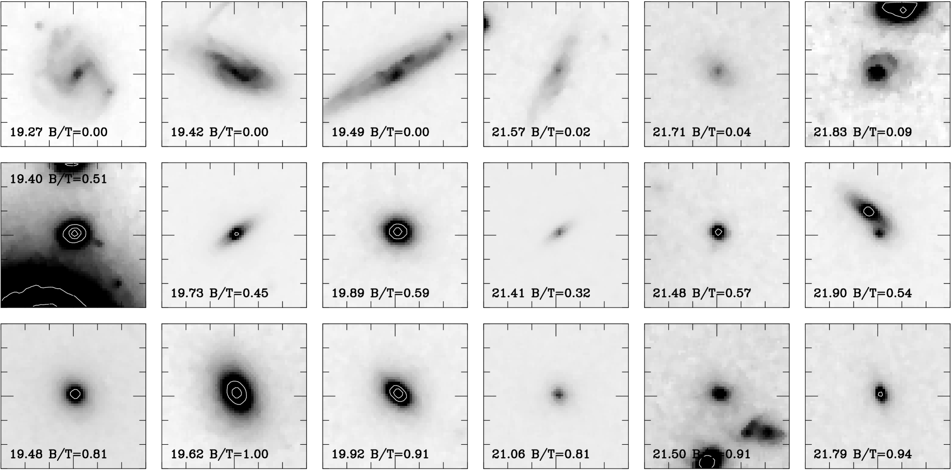
Figure 1.— Eighteen galaxies (9 bright and 9 faint) randomly selected from the cluster and field samples. Apparent $R_{702}$ magnitude and B/T values are shown in each panel. Each image is 6″ on a side, and contours are arbitrarily spaced. The top row shows galaxies with B/T$<0.1$, which are primarily spirals. Galaxies in the middle row have $0.4<B/T<0.6$, while the bottom row shows galaxies with B/T$>0.8$.

The visual classification of galaxies onto the revised Hubble system (or variations on it) has remained a central theme of recent morphological studies of distant galaxies with HST (Abraham et al. (1996b); Smail et al. (1997); van den Bergh (1997); Couch et al. (1998)). However, the high resolution and uniform quality data of these HST data has also encouraged the development of automated, machine-based techniques, which allow quantitative measures of morphology related to, but distinct from, the revised Hubble system (Schade et al. (1995); Abraham et al. (1996a); Odewahn et al. (1996); Naim et al. (1997); Marleau and Simard (1998); Brinchmann et al. (1998)). For the purposes of this paper we have chosen to follow the latter approach and hence analyse our sample using machine-based classifications based on fits to the two-dimensional surface brightness profiles of galaxies in the WFPC2 images.

To fit the data we use the iraf package gim2d v2.2.0, written by Luc Simard. The details of this program are given in Simard et al. (Simard et al. (2001)). gim2d fits the sky-subtracted surface brightness distribution of each galaxy with up to twelve parameters describing a “bulge” and “disk” component. The algorithm is similar to that used by Schade et al. (Schade et al. (1996a, b)), except that images are not symmetrized before fitting. Clearly, this two component model is a simplified approximation to the structure of real galaxies; furthermore, the distinction between a “disk” and “bulge” component is made purely on the surface brightness profile, and does not necessarily correspond to kinematically distinct components (see Simard et al. Simard et al. (2001)). For simplicity we nevertheless use the terms disk and bulge for these components in the following discussion.

The disk component is approximated by an exponential model, with parameters corresponding to the scale length, position angle and inclination. For the bulge, we fit a simple de Vaucouleurs profile instead of the more general Sérsic profile because the former generally provides a good fit to bright elliptical galaxies and the bulges of early-type spiral galaxies (de Jong (1994); Courteau et al. (1996); Andredakis (1998)). Sérsic profiles are more appropriate for the bulges of late-type galaxies (de Jong (1994)); however, these small bulges will be of low signal-to-noise in our images, making an accurate determination of the Sérsic index difficult.

gim2d searches the large parameter space of models using the Metropolis (Metropolis et al. (1953)) algorithm, which is inefficient but does not easily get trapped in local minima. An important step in this algorithm is an initial, broad sampling of the parameter space; we populate this space with 300 models.

We adopt a nominal magnitude limit of $R_{702}=23.0$ at $z=0.25$; galaxies brighter than this value are large enough and bright enough to be reliably classified. For $\Lambda$CDM, including small ($\mathrel{\raise 1.50696pt\hbox{$\scriptstyle<$}\kern-6.00006pt\lower 1.72218pt\hbox{{$\scriptstyle\sim$}}}0.1$ mag) k-corrections, this corresponds to $\hbox{$\rm\thinspace M_{702}$}=-18.2+5\log{h_{50}}$, approximately $M_{R}\sim-18.0+5\log{h_{50}}$, 4.6 magnitudes below $M_{R}^{\ast}$ (Blanton et al. (2001)). Accounting for the range of redshifts spanned by our clusters, we adjust this limit so that the data are matched to the same limiting absolute magnitude. Therefore, for our most nearby cluster A 2218 ($z=0.17$) we use a magnitude limit of $R_{702}=22.1$, while for the most distant cluster Cl 1444+63 ($z=0.29$) we use $R_{702}=23.45$. We use a field galaxy sample cut at the corresponding $I_{814}$ limit based on a typical color of $(R_{702}-I_{814})\sim 0.4$, as discussed in §2.1.

We start from an initial list of sources from the SExtractor catalogs which are more than 3″ from a WFC chip edge, are entirely contained within the trimmed image, and are brighter than the relevant magnitude limit for the cluster listed in Table 1. We then exclude sources with half-light radii less than 0$\farcs$15, which are stars, and giant arcs in the High–$L_{X}$ sample. The exclusion of the arcs, which are clearly background galaxies, has no significant impact on our results because the background contamination in the High–$L_{X}$ clusters is very small.

For each galaxy, we run gim2d using the pixel membership defined by SExtractor’s segmentation image. This provides best fitting estimates and errors for the bulge and disk components of the galaxy. It is quite remarkable how good a fit this simple, two component model provides to the majority of the galaxies; we find reduced $\chi^{2}$ values between one and two for more than 90 per cent of the galaxies. No restrictions regarding goodness of fit or symmetry are imposed in the subsequent analysis. From the fitted parameters we calculate B/T, the fraction of the luminosity in the bulge, relative to the total luminosity. This parameter is known to correlate with Hubble type (Simien and de Vaucouleurs (1986)), though there is considerable scatter about the mean relation. The uncertainties in B/T are determined from Monte Carlo simulation in the GIM2D software, and have a median value of 0.07.

To ensure consistency with the results of the photometric fitting, the total magnitude for each galaxy is taken to be the total flux in the model, as computed by the GIM2D software. These total fluxes are systematically brighter than the Kron-type magnitudes calculated with SExtractor, by $\sim 0.15$ mag, with a dispersion of $\sim 0.25$ mag. The offset is larger, $\sim 0.25$ mag, for the brightest galaxies, $R_{702}<18$; fainter than this magnitude there is no significant trend with magnitude.

In Figure  1 we show 6″ images of 18 galaxies, randomly selected from the Low–$L_{X}$, High–$L_{X}$ and MDS samples. The $R_{702}$ magnitude and B/T value are printed in each panel. In the top row, three bright and three faint galaxies with B/T$<0.1$ are shown. This regime of B/T consistently selects disk-dominated galaxies, despite the common occurrence of spiral arms and bright HII regions. This is not too surprising, since the disk decomposition is based on the assumption that the disk surface brightness follows an exponential profile, as is the case in the majority of spiral galaxies (e.g. de Jong 1996). In the next two rows, we show images of galaxies with $0.4<B/T<0.6$, and $B/T>0.8$, respectively. This allows the reader to associate B/T measurements with the more traditional morphology of the galaxy (see also Marleau & Simard et al. 1998; Tran et al. 2001; Simard et al. 2001).

3. Results and Analysis

3.1. Morphological Distributions

The luminosity functions of the Low–$L_{X}$ and High–$L_{X}$ samples are shown in Figure 2, normalized to the average number of galaxies per cluster above the magnitude limit in the High–$L_{X}$ sample. The background subtracted is also shown in this Figure. We find no gross dependence of the luminosity function on environment, in agreement with the results at lower redshift from Zabludoff & Mulchaey (Zabludoff and Mulchaey (2000)). We can therefore compare the distributions of B/T in the High–$L_{X}$ and Low–$L_{X}$ clusters, including all galaxies brighter than $\hbox{$\rm\thinspace M_{702}$}=-18.2+5\log{h_{50}}$ ($\mathrel{\raise 1.50696pt\hbox{$\scriptstyle>$}\kern-6.00006pt\lower 1.72218pt\hbox{{$\scriptstyle\sim$}}}0.01L^{\ast}$). Since the redshift distributions of the clusters (Table 1) and the luminosity functions of their constituent galaxies are very similar, any differences seen in these distributions must therefore be related (though not necessarily directly, as we discuss in §3.2) to the difference in X-ray luminosity, cluster mass or local galaxy density.

To correct for the fore- and background contamination of the clusters, we first consider the distribution of B/T in the field galaxy sample from the eight MDS fields, shown in the top left panel of Figure 3. The distribution has a strong peak at B/T$=0$, and 65$\pm$9 per cent (error from the field-to-field standard deviation) of all galaxies have B/T $<0.4$; i.e., they are disk-dominated. In the remaining panels on the left side of Figure 3 we show the distribution of B/T in each of the eight Low–$L_{X}$ clusters (dotted histograms). We correct for foreground and background contamination by subtracting the mean field B/T distribution; the corrected distribution is shown as the solid histograms. In most cases, the effect of background contamination is small, and generally serves to reduce the fraction of disk-dominated galaxies by only a few per cent. In most clusters the field-corrected B/T distribution is reminiscent of that seen for the field population, with a comparatively flat distribution except for a pronounced peak in several clusters at B/T $\sim 0$. The B/T distributions for the individual Low–$L_{X}$ clusters are statistically consistent with the mean distribution, so there is no significant variation from cluster to cluster.

Fig. 2.— The luminosity functions of galaxies in the Low–$L_{X}$ (heavy, solid line) and High–$L_{X}$ (heavy, dotted line) clusters after field correction, both renormalized to the average number of galaxies per cluster in the High–$L_{X}$ sample. The error bars include the uncertainty in the background correction; the field component subtracted from the Low–$L_{X}$ and High–$L_{X}$ samples are shown as the thin solid and thin dotted lines, respectively.

     

Figure 3.— Left: The distribution of B/T in the eight Low–$L_{X}$ clusters, and the mean distribution of the MDS field sample. For the eight clusters, the dotted histograms show the distribution of all galaxies, and the solid histograms are corrected for fore- and background contamination by subtracting the field distribution. Right: The B/T distributions of the High–$L_{X}$ clusters.

The B/T distributions for the clusters of the High–$L_{X}$ sample are shown in the right hand panels of Figure 3, again with and without field correction (this is less important for this sample than for the Low–$L_{X}$ clusters). In general, the High–$L_{X}$ sample shows more marked differences from the field population than the Low–$L_{X}$ systems. In particular, most of the clusters lack large numbers of galaxies with B/T $\sim 0$ and instead show a broad peak of bulge-strong galaxies with B/T $\sim 0.5$. There are three notable exceptions to this general statement: A 963, A 267 and A 383, which all show a peak at B/T=0, and distributions which are broadly similar to the Low–$L_{X}$ clusters. We discuss these three discrepant clusters in more detail in §4.

The simplest way to characterise the morphological mix of the clusters is to evaluate the fraction of disk-dominated galaxies in each cluster after field-correction. We arbitrarily define a disk-dominated galaxy to have B/T$<0.4$; however, our qualitative conclusions are unchanged for any definition ranging from B/T$<0.1$ to B/T$<0.5$. In Figure 4 we show the fractions of disk-dominated galaxies in the clusters as a function of their X-ray luminosities. The disk-dominated galaxy fraction in the field sample has a mean of 0.65 and we show this for reference; along with the 1-$\sigma$ field-to-field standard deviation of 0.09. The error-weighted mean fraction of disk-dominated galaxies in the High–$L_{X}$ clusters is 0.23$\pm 0.10$, where the quoted uncertainty represents the 1-$\sigma$ standard deviation from cluster to cluster. This 10 per cent variation is well above the statistical uncertainty, and is due to the three clusters noted earlier (A 963, A 267 and A 383) which have unusually high fractions of disk-dominated galaxies. For the Low–$L_{X}$ cluster sample the spread in B/T is similar, but the disk-dominated fraction is much higher on average, at 0.40$\pm 0.09$. However, even in these systems the disk fraction is still significantly lower than the general field. This suggests that the processes influencing galaxy morphology can effect galaxies inhabiting structures less massive than X-ray luminous clusters, in agreement with the results of Tran et al. (Tran et al. (2001)). However, we caution that the field galaxy sample is magnitude limited, and therefore has absolute magnitude and redshift distributions different from those of the volume-limited cluster samples. In particular, we expect the redshift distribution of the field sample to peak at $z\approx 0.55$ (Crampton et al. (1995)).

Fig. 4.— The fraction of disk-dominated galaxies (those with B/T$<$0.4) in the Low–$L_{X}$  and High–$L_{X}$ samples as a function of the cluster X-ray luminosities (open circles). Error bars on the data points are 1-$\sigma$ bootstrap estimates, and include the uncertainty in the background correction. The solid diamonds show the error-weighted mean fractions for the combined Low–$L_{X}$ and High–$L_{X}$ samples, with an error bar which represents the 1$-\sigma$ standard deviation in this fraction from cluster to cluster (i.e. it is not the error on the mean). The solid line is the corresponding fraction in the field population, and the dashed lines show the 1-$\sigma$ field-to-field standard deviation of this quantity.

3.2. Local or global environment?

The results of the previous section show that the distribution of galaxy morphologies is different in the Low–$L_{X}$ and High–$L_{X}$ cluster samples. We now wish to test whether this is due to differences in the local galaxy environment, or whether it instead reflects the influence of the global environment on the galaxy populations.

The clusters in the two samples we analyse have significant differences in their physical properties, with the mean $L_{X}$ of the High–$L_{X}$ sample a factor of $\sim 30$ times higher than that of the Low–$L_{X}$ sample. This corresponds to a difference of a factor $\sim 5$ in mass, or a factor of $\sim 2$ in virial radius (from $M\propto L^{1/2}\propto R_{\rm vir}^{3}$; e.g. see Babul et al.  Babul et al. (2001)). As the galaxy samples in the High–$L_{X}$ and Low–$L_{X}$ clusters are selected from the same physical region ($\sim 3\arcmin$ in diameter or $\sim 1h_{50}^{-1}$ Mpc for a $\Lambda$CDM cosmology), the galaxies in the Low–$L_{X}$ sample are selected from a region covering a substantially larger fraction of the virial radius of the clusters, compared with the High–$L_{X}$ sample. Within relaxed systems local density is strongly correlated with radius normalized to the virial radius (Carlberg et al. (1997)); we therefore expect that the typical galaxy density in the regions of the High–$L_{X}$ and Low–$L_{X}$ clusters analysed here will differ. Thus, if a strong morphology–density relation exists in the clusters (Dressler (1980); Postman and Geller (1984); Tran et al. (2001)), the systematic variation in the local galaxy density between the two samples will lead to differences in the apparent morphological mix.

Fig. 5.— Top panel: The distribution of projected local galaxy surface density in the Low–$L_{X}$ (solid line) and High–$L_{X}$ (dotted line) samples. Bottom panel: The fraction of galaxies with B/T$<$0.4 as a function of projected local galaxy density. The values are corrected for background contamination as described in the text. The field fraction (which corresponds to $\Sigma_{\rm local}\sim 0$) is shown as the star at an arbitrary density for display purposes. The circles and triangles correspond to the Low–$L_{X}$ and High–$L_{X}$ samples, respectively. Bin sizes are adaptively varied so that each includes 75 galaxies; the horizontal error bar shows the bin span, and the point represents the median. Vertical error bars are determined from bootstrap resampling which accounts for the uncertainty in the background correction.

The local projected galaxy density around each galaxy is computed in a manner similar to that of Dressler (Dressler (1980)). The five nearest neighbor galaxies are found, down to the appropriate limiting magnitude (see §2.4) and the encompassing area is taken to be a circle which extends out to the most distant neighbor (correctly accounting for the smaller area available for galaxies near the boundary of the WFC mosaic). We choose the fifth nearest neighbor, rather than the more traditional choice of the tenth, since the latter choice results in an uncomfortably large smoothing scale, relative to the small area of the WFC images. The average field density computed at the appropriate magnitude limit ($\Sigma_{f}=5.4$ arcmin^-2 at $I_{814}=22.5$) is subtracted to give the local density $\Sigma_{\rm local}$, which is converted to physical units ($h_{50}^{2}$ Mpc^-2) assuming a $\Lambda$CDM cosmology. When computing the projected densities, all of the surrounding galaxies in the photometric catalog above the magnitude limit are considered, though we have only determined morphologies for galaxies which are well clear of chip boundaries. We have not accounted for the fact that the trimmed chip images do not exactly join, so local densities near the common boundary of two WFC chips will be slightly underestimated.

The contribution of the background to the observed B/T distribution depends on the local projected density of galaxies under consideration; in denser regions, the background correction will be proportionally smaller. For the total cluster sample, we computed the mean projected field density from the MDS, $\Sigma_{f}$, to the appropriate magnitude limit for each cluster, and subtracted the corresponding number of galaxies. For galaxies within a restricted range of projected densities, we scale the MDS B/T distribution appropriately so that a fraction $f=\Sigma_{f}/(\Sigma_{f}+\bar{\Sigma})$ of the galaxy population is statistically subtracted from the observed B/T distribution, where $\bar{\Sigma}$ is the median, background-corrected density of the galaxy subsample. For $\bar{\Sigma}\sim 25h_{50}^{2}$ Mpc^-2, $f\sim 60$ per cent, while for $\bar{\Sigma}\sim 250h_{50}^{2}$ Mpc^-2, $f\sim 10$ per cent.

In the top panel of Figure 5 we show the $\Sigma_{\rm local}$ distributions of the Low–$L_{X}$ and High–$L_{X}$ samples. As expected, most of the galaxies in the Low–$L_{X}$ sample are drawn from regions of much lower galaxy density than seen for the bulk of the galaxies in the High–$L_{X}$ sample. Note that the typical densities in the High–$L_{X}$ sample are much larger than those shown in Dressler (Dressler (1980)), since we are including galaxies about 2.5 magnitudes less luminous than in Dressler’s study.

Fig. 6.— The distribution of B/T ratios is shown for low (lowest 5-25 percentile) and high (highest 5-25 percentile) density regions separately, as indicated. The Low–$L_{X}$ cluster data are shown in the top panel, and the High–$L_{X}$ cluster data are shown in the bottom panel. Uncertainties are 1$-\sigma$ and include the error in background subtraction.

The morphology-density relation is shown in the bottom panel of Figure 5. We use an adaptive bin size so that each bin contains 75 galaxies, and compute the field-corrected fraction of those that are disk-dominated, B/T$<0.4$ (as this definition of disk-dominated is arbitrary we will consider the full B/T distribution as a function of density below). In the individual cluster samples there is only weak evidence for a morphology–density relation due to the small samples and limited dynamic range in density. In Figure 6 we compare the background-subtracted distribution of B/T in low (5-25 percentile) and high (75-95 percentile) density regions within the individual Low–$L_{X}$ and High–$L_{X}$ samples. The corresponding density limits in each sample are also shown in Figure 6. This compares galaxies in well separated density ranges above and below the mean of the sample, while avoiding the extreme tails of the distribution. No statistically significant difference can be seen between the low and high density regimes, in either cluster sample. There is an indication, in the High–$L_{X}$ clusters, that the lowest density galaxies are distributed toward lower B/T, but the reduced $\chi^{2}$ statistic for the difference between these two distributions, accounting for the uncertainty in background subtraction, is only 1.2. The T–$\Sigma$ is clearly weak, at best; this can be attributed partly to the limited dynamic range of densities explored; HST imaging over a wider field would allow the extension of the analysis of the High–$L_{X}$ clusters to much lower densities, and improve the comparison.

There is some evidence from Figure 5 that, at a given overdensity, disk-dominated galaxies are more common in the Low–$L_{X}$ clusters. We investigate this possibility by restricting the galaxy samples in both High–$L_{X}$ and Low–$L_{X}$ clusters to a common density range where both samples have good statistics, $\Sigma_{\rm local}=50$–200. In this density range, there is good overlap between the two datasets, and limited gradient in morphological composition. Although this density range is still fairly large, our results do not qualitatively change as this interval is reduced, at the necessary expense of lower statistical significance.

The B/T distributions in the High–$L_{X}$ and Low–$L_{X}$ clusters, restricted to $\Sigma_{\rm local}=50$–200, are shown in Figure 7. The two distributions appear to differ, with a relative excess of galaxies in the High–$L_{X}$ sample with B/T$\sim$0.5, and a corresponding deficit of those with B/T $\sim 0$. A statistical comparison of the two normalised distributions gives a reduced $\chi^{2}$ of 3.1 and a corresponding likelihood of 98%. This difference is much more pronounced and significant (99.99% likelihood) if we exclude the three unusual High–$L_{X}$ clusters discussed in §3.1; however, we are reluctant to do so without identifying the origin of the difference between these and the majority of the High–$L_{X}$ systems. We also reemphasize that the $\chi^{2}$ test is sensitive to the binning of the data and thus does not provide a complete statistical description of the difference between the samples.

4. Discussion

From Figures 3 and 4, it is evident that all of the Low–$L_{X}$ clusters have similar galaxy morphology distributions; all eight clusters are dominated by galaxies with B/T$\approx 0$, and are statistically indistinguishible from the mean B/T distribution of the combined sample. Most of the High–$L_{X}$ clusters differ from this distribution, as they are dominated by galaxies with intermediate B/T. The exceptions are three clusters, A 963, A 267 and A 383, which have B/T distributions more similar to those found in the Low–$L_{X}$ clusters. There is nothing strikingly unusual about the morphology of these three clusters; all are dominated by a single cD galaxy and do not show obvious signs of irregularity. The redshifts of these three clusters are not at either extreme of the distribution, nor are the galaxy luminosity functions, or distributions of local projected density, significantly different from that of the average High–$L_{X}$ cluster.

One possible explanation for the difference could be that these three clusters are less massive than the other High–$L_{X}$ clusters, and that their X-ray luminosities are unusually high, or overestimated. Alternatively, if the clusters have an unusually large number density of fore- and background galaxies along the line of sight, the background correction will have been underestimated. However, the local galaxy density distribution of the three clusters is indistinguishible from the High–$L_{X}$ cluster average; that is, the galaxy density is as high as we expect for the cluster’s luminosity. It would seem, therefore, that both the luminosity and the density would have to be artificially enhanced for these explanations to work; this would be an uncomfortable coincidence. It therefore appears that galaxy morphology is sensitive to factors other than just local density or X-ray luminosity, though it is not clear what they are.

Fig. 7.— The B/T distribution for galaxies with $\Sigma_{\rm local}=50$–200 $h_{50}^{2}$ Mpc^-2. The solid and dotted histograms correspond to the Low–$L_{X}$ and High–$L_{X}$ samples, respectively.

Putting aside for the moment the intrinsic variation in the High–$L_{X}$ sample, we can explore differences in the average properties of the High–$L_{X}$ and Low–$L_{X}$ clusters. There is some evidence that disk-dominated galaxies are relatively more common in the Low–$L_{X}$ clusters, at fixed overdensity, relative to the High–$L_{X}$ clusters (Figure 7). Although this result is of marginal statistical significance, it is still of interest to investigate which physical process could give rise to the effect. In currently popular models of galaxy formation, bulge-dominated galaxies are generally created in one of two ways. The first is by the merger of two galaxies, in which some or all of the baryonic material (from the progenitor bulges and disks) is converted into a new bulge component. In this case, differences in the bulge luminosity function will reflect differences in the galaxy merger histories. Alternatively, a bulge-dominated galaxy can be created by reducing the stellar mass of the disk component, either by destroying it (for example, through harassment) or by causing it to fade sufficiently following the cessation of star formation (as might be expected if ram pressure stripping removes all the gas from the disk). In this case, the bulge luminosity function should be unaffected by the efficiency of the destruction process, but the B/T measure will increase as the disk fades or is destroyed. We will attempt to distinguish between these two possibilities by examining the relationship between bulge luminosity and B/T in the two cluster samples.

     

Figure 8.— Left: The luminosity function of the bulge component, in the Low–$L_{X}$ sample (heavy, solid line) and the High–$L_{X}$ sample (heavy, dotted line), restricted to regions of overdensity $50<\Sigma_{\rm local}<200$. $\phi$(M) is normalised to the average number of galaxies per cluster in the High–$L_{X}$ sample, restricted to this density range. The thin solid and dotted lines show the subtracted background component. Right: The same, but for the disk components.

We show the bulge and disk luminosity functions separately in Figure 8, for those galaxies from Low–$L_{X}$ and High–$L_{X}$ samples lying within the density range $\Sigma_{\rm local}=50$–200. The luminosity functions are normalized to the average number of galaxies in this density range per cluster in the High–$L_{X}$ sample. While the disk luminosity functions appear to be very similar in both cluster samples, there is an indication (not statistically significant, however) that the bulge luminosity function is steeper in the High–$L_{X}$ clusters; i.e., there is a higher proportion of low-luminosity bulges compared with the Low–$L_{X}$ sample. This suggests that the difference in B/T distributions is reflecting a difference in the properties of the bulges, rather than the disks. With some effort, this can be seen more clearly in the correlation of B/T with disk or bulge luminosity, shown in Figure 9. We again restrict the galaxy population to those with $\Sigma_{\rm local}=50$–200, to minimize morphology-density effects. Concentrating first on the top panels, we see the correlation between B/T and bulge luminosity, for the Low–$L_{X}$ and High–$L_{X}$ samples separately. Galaxies with B/T$<0.1$ have been arbitrarily plotted at B/T$=0.1$ to make them visible in this logarithmic plot. Note also that the shape of the sample luminosity limit, combined with the shape of the luminosity function, gives rise to some of the structure seen in this figure. It is clear (as it is in Figure 7) that the Low–$L_{X}$ clusters are dominated by galaxies with low B/T, while this is much less the case in the High–$L_{X}$ clusters. We can now explore the two scenarios described above. If galaxy disks are preferentially stripped, or otherwise fade, in the High–$L_{X}$ clusters, the galaxy density will be shifted directly upward in this figure, relative to the Low–$L_{X}$ distribution (see the arrows labelled “S”). This would serve to push many of the galaxies with B/T$<0.2$, which are mostly faint, below our luminosity limit. In this respect, such a mechanism could provide a viable explanation of the difference in galaxy distributions seen in these top figures. However, if we now look at the bottom panels, it can be seen that this explanation is unlikely. In these figures, we plot disk luminosity as the x-axis. Here, it is clear that the faint end of the disk luminosity function is primarily defined by galaxies with B/T$<0.2$. If these disks were to fade beyond the luminosity limit, the disk luminosity function would necessarily become much shallower, and this does not appear to be the case (Figure  8). Instead, the faint end of the disk luminosity function in the High–$L_{X}$ clusters is relatively more populated by galaxies with B/T$\sim 0.5$ and disk luminosities roughly equivalent to the disk luminosities of the B/T$\sim 0$ population in the Low–$L_{X}$ clusters.

On the other hand, if the difference between the Low–$L_{X}$ and High–$L_{X}$ clusters is due to the fact that the bulges are systematically brighter in the High–$L_{X}$ clusters, due perhaps to a more extensive merger history, galaxies in these panels will move diagonally, as indicated by the arrows labelled “M”. This explanation appears consistent with the observations. The B/T$<0.2$ population which dominates the Low–$L_{X}$ clusters can be translated in the sense of brightening their bulges at constant disk luminosities, to reproduce the distribution seen in the High–$L_{X}$ clusters.

We conclude that is unlikely the B/T$\sim 0.5$ galaxies in the High–$L_{X}$ clusters have been formed from a process which operates uniquely in this environment by stripping or otherwise destroying the disk in a lower B/T system. Rather, the results seem to suggest that there are differences in bulge growth in the Low–$L_{X}$ and High–$L_{X}$ samples. This provides quantitative support for the suggestion by Dressler (Dressler (1980)), that the early-type galaxies in clusters cannot all be formed by destroying the disks of a normal population of late-type galaxies. However, this is not evidence that ram pressure stripping (or other processes with similar effect) do not take place at all; at least, they could play a strong role in establishing the local morphology-density relation. But the difference between the T–$\Sigma$ for Low–$L_{X}$ and High–$L_{X}$ clusters indicates that there are other processes at work.

     

     

Figure 9.— Top: The correlation between B/T and bulge luminosity is shown for galaxies in the High–$L_{X}$ clusters (left) and the Low–$L_{X}$ clusters (right), after background subtraction. The sample is restricted to those galaxies in the local projected density range $\Sigma_{\rm local}=50$–200 $h_{50}^{2}$ Mpc^-2. The density of galaxies in this plane is represented as a contour plot; the contours are equally spaced in intervals of 5 galaxies per cell (starting with 1), where a cell is 1 mag and 0.1 in B/T. Galaxies with B/T$<0.1$ are arbitrarily fixed at B/T=0.1 to be visible in these plots. The short-dashed lines show the bulge luminosity of an M^∗ galaxy, and a galaxy three magnitudes fainter, as a function of B/T, for reference. The long-dashed line represents the luminosity limit of the sample. The arrows labelled “S” and “M” show the magnitude and direction a galaxy with B/T=0.1 would move, if its disk faded by one magnitude (stripping: S) or its bulge brightened by one magnitude (merging: M). Bottom: Same as the top panel, but for the correlation between B/T and disk luminosity. Galaxies with B/T$>0.9$ are arbitrarily fixed at B/T$=0.9$ to be visible in these plots.

5. Conclusions

We have presented an HST-based morphological analysis of galaxies in clusters from two samples at $z\sim 0.25$. The two data sets are extremely well matched in the properties and quality of their data; all observations are 3-orbit HST exposures in the F702W filter, and both cluster samples have a similar mean redshift and small redshift range, thus minimizing differences in k-corrections and absolute magnitude limits. The only significant difference between the samples is the X-ray luminosity of the clusters contained in them; the clusters in the Low–$L_{X}$ sample have $L_{X}$(0.1–2.4 keV)=0.15–1.5$\times 10^{44}$ ergs s^-1, while the High–$L_{X}$ clusters have $L_{X}$(0.1–2.4 keV)$\geq 10^{45}$ ergs s^-1. These data are therefore ideal for testing the dependence of galaxy morphology on local density and the global environment. We summarize our findings as follows:

• Within a fixed physical region ($\sim 1h_{50}^{-1}$ Mpc diameter), the fraction of disk-dominated galaxies is strongly dependent on $L_{X}$. In the High–$L_{X}$ sample, the fraction of galaxies with B/T$<0.4$ is 0.25$\pm 0.10$, while in the Low–$L_{X}$ sample it is 0.44$\pm 0.07$.

• In both cluster samples, the fraction of galaxies with B/T$<0.4$ is significantly lower than the fraction of such galaxies in the field, 0.65$\pm 0.09$ (where the uncertainty represents the field-to-field variation). The origin of this discrepancy is, however, unclear because the comparison is between a volume-limited sample at $z\sim 0.25$ (the clusters) and a magnitude-limited one with a broad redshift distribution peaked at $z\sim 0.55$ (the field).

• There is a dependence of the typical B/T of a galaxy on its local projected galaxy density. This is partly responsible for the above result, as galaxies in the High–$L_{X}$ clusters are generally located in denser environments. However, when we compare galaxies at similar local densities in the Low–$L_{X}$ and High–$L_{X}$ samples, small differences persist, with the High–$L_{X}$ clusters showing an excess of bulge-strong galaxies compared to the Low–$L_{X}$ sample. This difference is moderately significant, with confidence limits of 98% (as determined by a $\chi^{2}$ test, which is sensitive to how the data are binned).

• To investigate this behaviour in more detail we focus on the bulge luminosity function in the two samples. We find some evidence for a difference in the bulge luminosity function of galaxies between the Low–$L_{X}$ and High–$L_{X}$ clusters when we restrict the comparison to galaxies with local densities between 50 and 200 $h_{50}^{2}$ Mpc^-2, although the difference is not highly statistically significant.

• Three of the High–$L_{X}$ clusters show B/T distributions which are more similar to the average Low–$L_{X}$ B/T distribution than the majority of High–$L_{X}$ clusters. Galaxy morphology therefore appears to depend on another, unknown parameter, besides local density and X-ray luminosity.

These observations suggest that the factors influencing galaxy morphlogy are: 1) efficient in relatively low-mass clusters; and 2) influence the luminosity of the bulge component, and not the disk alone. The most likely interpretation in our opinion is that the merger histories of galaxies in low and high mass clusters are different, in that merging has played a larger role for galaxies 1–3 magnitudes below $\sim L^{\ast}$ in more massive clusters. This might be expected from models of hierarchical cluster growth (Lacey and Cole (1994); Kauffmann (1996)), since the merger history of massive clusters tends to be more extended. On the other hand, galaxy-galaxy mergers are uncommon in regions of high velocity dispersion, and it is unclear what variation in the bulge luminosity function would be predicted by the models.

References

- Abell (1965) Abell, G. O.: 1965, ARA&A 3, 1
- Abraham et al. (1996a) Abraham, R. G., Tanvir, N. R., Santiago, B. X., Ellis, R. S., Glazebrook, K., and van den Bergh, S.: 1996a, MNRAS 279, L47
- Abraham et al. (1996b) Abraham, R. G., van den Bergh, S., Glazebrook, K., Ellis, R. S., Santiago, B. X., Surma, P., and Griffiths, R. E.: 1996b, ApJS 107, 1
- Allen and Fabian (1998) Allen, S. W. and Fabian, A. C.: 1998, MNRAS 297, L57
- Andredakis (1998) Andredakis, Y. C.: 1998, MNRAS 295, 725
- Andreon (1998) Andreon, S.: 1998, ApJ 501, 533
- Babul et al. (2001) Babul, A., Balogh, L., M., Lewis, G. F., and Poole, G. B.: 2001, MNRAS pp in press, astro–ph/0109329
- Bahcall (1977) Bahcall, N. A.: 1977, ApJL 218, 93
- Balogh et al. (1999) Balogh, M. L., Morris, S. L., Yee, H. K. C., Carlberg, R. G., and Ellingson, E.: 1999, ApJ 527, 54
- Balogh et al. (2000) Balogh, M. L., Navarro, J. F., and Morris, S. L.: 2000, ApJ 540, 113
- Balogh et al. (1998) Balogh, M. L., Schade, D., Morris, S. L., Yee, H. K. C., Carlberg, R. G., and Ellingson, E.: 1998, ApJL 504, 75
- Bardeen et al. (1986) Bardeen, J. M., Bond, J. R., Kaiser, N., and Szalay, A. S.: 1986, ApJ 304, 15
- Barnes (1992) Barnes, J. E.: 1992, ApJ 393, 484
- Baugh et al. (1996) Baugh, C. M., Cole, S., and Frenk, C. S.: 1996, MNRAS 283, 1361
- Bertin and Arnouts (1996) Bertin, E. and Arnouts, S.: 1996, A&AS 117, 393
- Blanton et al. (2001) Blanton, M. R., Dalcanton, J., Eisenstein, D., Loveday, J., Strauss, M. A., SubbaRao, M., Weinberg, D. H., and the Sloan collaboration: 2001, AJ 121, 2358
- Bravo-Alfaro et al. (2000) Bravo-Alfaro, H., Cayatte, V., van Gorkom, J. H., and Balkowski, C.: 2000, AJ 119, 580
- Brinchmann et al. (1998) Brinchmann, J., Abraham, R., Schade, D., Tresse, L., Ellis, R. S., Lilly, S., Le Fevre, O., Glazebrook, K., Hammer, F., Colless, M., Crampton, D., and Broadhurst, T.: 1998, ApJ 499, 112
- Carlberg et al. (1997) Carlberg, R. G., Yee, H. K. C., and Ellingson, E.: 1997, ApJ 478, 462
- Cole (1991) Cole, S.: 1991, ApJ 367, 45
- Cooray (1999) Cooray, A. R.: 1999, MNRAS 307, 841
- Couch et al. (1998) Couch, W. J., Barger, A. J., Smail, I., Ellis, R. S., and Sharples, R. M.: 1998, ApJ 497, 188
- Couch et al. (1994) Couch, W. J., Ellis, R. S., Sharples, R. M., and Smail, I.: 1994, ApJ 430, 121
- Courteau et al. (1996) Courteau, S., de Jong, R. S., and Broeils, A. H.: 1996, ApJL 457, L73
- Crampton et al. (1995) Crampton, D., Le Fevre, O., Lilly, S. J., and Hammer, F.: 1995, ApJ 455, 96
- de Jong (1994) de Jong, R. S.: 1994, Ph.D. thesis, Kapteyn Astronomical Inst., (1994)
- de Jong (1996) de Jong, R. S.: 1996, A&ASS 118, 557
- Diaferio et al. (2001) Diaferio, A., Kauffmann, G., Balogh, M. L., White, S. D. M., Schade, D., and Ellingson, E.: 2001, MNRAS 323, 999
- Dressler (1980) Dressler, A.: 1980, ApJ 236, 351
- Dressler et al. (1997) Dressler, A., Oemler, A., Couch, W. J., Smail, I., Ellis, R. S., Barger, A., Butcher, H. R., Poggianti, B. M., and Sharples, R. M.: 1997, ApJ 490, 577
- Dressler et al. (1985) Dressler, A., Thompson, I. B., and Shectman, S.: 1985, ApJ 288, 481
- Ebeling et al. (1998) Ebeling, H., Edge, A. C., Bohringer, H., Allen, S. W., Crawford, C. S., Fabian, A. C., Voges, W., and Huchra, J. P.: 1998, MNRAS 301, 881
- Ebeling et al. (1996) Ebeling, H., Voges, W., Bohringer, H., Edge, A. C., Huchra, J. P., and Briel, U. G.: 1996, MNRAS 281, 799
- Fabricant et al. (2000) Fabricant, D., Franx, M., and van Dokkum, P.: 2000, ApJ 539, 577
- Farouki and Shapiro (1982) Farouki, R. T. and Shapiro, S. L.: 1982, ApJ 259, 103
- Fasano et al. (2000) Fasano, G., Poggianti, B. M., Couch, W. J., Bettoni, D., Kjaergaard, P., and Moles, M.: 2000, ApJ 542, 673
- Fukugita et al. (1995) Fukugita, M., Shimasaku, K., and Ichikawa, T.: 1995, PASP 107, 945
- Giovanelli and Haynes (1985) Giovanelli, R. and Haynes, M.: 1985, ApJ 292, 404
- Gunn and Gott (1972) Gunn, J. E. and Gott, J. R. I.: 1972, ApJ 176, 1
- Hubble and Humason (1931) Hubble, E. and Humason, M. L.: 1931, ApJ 74, 43
- Hubble (1922) Hubble, E. P.: 1922, ApJ 56, 162
- Hubble (1926) Hubble, E. P.: 1926, ApJ 64, 321
- Jones et al. (2000) Jones, L., Smail, I., and Couch, W. J.: 2000, ApJ 528, 118
- Kauffmann (1996) Kauffmann, G.: 1996, MNRAS 281, 487
- Kauffmann et al. (1993) Kauffmann, G., White, S. D. M., and Guiderdoni, B.: 1993, MNRAS 264, 201
- Kodama and Smail (2001) Kodama, T. and Smail, I.: 2001, MNRAS 326, 637
- Kuntschner and Davies (1998) Kuntschner, H. and Davies, R. L.: 1998, MNRAS 295, L29
- Lacey and Cole (1994) Lacey, C. and Cole, S.: 1994, MNRAS 271, 676
- Larson et al. (1980) Larson, R. B., Tinsley, B. M., and Caldwell, C. N.: 1980, ApJ 237, 692
- Lewis et al. (1999) Lewis, A. D., Ellingson, E., Morris, S. L., and Carlberg, R. G.: 1999, ApJ 517, 587
- Markevitch (1998) Markevitch, M.: 1998, ApJ 504, 27
- Marleau and Simard (1998) Marleau, F. R. and Simard, L.: 1998, ApJ 507, 585
- Metcalfe et al. (2001) Metcalfe, N., Shanks, T., Campos, A., McCracken, H. J., and Fong, R.: 2001, MNRAS 323, 795
- Metropolis et al. (1953) Metropolis, N., Rosenbluth, A., Rosenbluth, M., Teller, A., and Teller, E.: 1953, Journal of Chemical Physics 21, 1087
- Moore et al. (1999) Moore, B., Lake, G., Quinn, T., and Stadel, J.: 1999, MNRAS 304, 465
- Morgan (1961) Morgan, W. W.: 1961, Proc. Nat. Acad. Sci. 47, 905
- Moss and Whittle (2000) Moss, C. and Whittle, M.: 2000, MNRAS 317, 667
- Naim et al. (1997) Naim, A., Ratnatunga, K. U., and Griffiths, R. E.: 1997, ApJS 111, 357
- Narayanan et al. (2000) Narayanan, V. K., Berlind, A. A., and Weinberg, D. H.: 2000, ApJ 528, 1
- Nulsen (1982) Nulsen, P. E. J.: 1982, MNRAS 198, 1007
- Odewahn et al. (1996) Odewahn, S. C., Windhorst, R. A., Driver, S. P., and Keel, W. C.: 1996, ApJL 472, L13
- Osterbrock (1960) Osterbrock, D. E.: 1960, ApJ 132, 325
- Ostrander et al. (1998) Ostrander, E. J., Nichol, R. C., Ratnatunga, K. U., and Griffiths, R. E.: 1998, AJ 116, 2644
- Poggianti et al. (1999) Poggianti, B. M., Smail, I., Dressler, A., Couch, W. J., Barger, A. J., Butcher, H., Ellis, R. S., and Oemler, A.: 1999, ApJ 518, 576
- Postman and Geller (1984) Postman, M. and Geller, M. J.: 1984, ApJ 281, 95
- Ratnatunga et al. (1999) Ratnatunga, K. U., Griffiths, R. E., and Ostrander, E. J.: 1999, AJ 118, 86
- Roche et al. (1996) Roche, N., Ratnatunga, K., Griffiths, R. E., Im, M., and Neuschaefer, L.: 1996, MNRAS 282, 1247
- Roos and Norman (1979) Roos, N. and Norman, C. A.: 1979, A&A 76, 75
- Saglia et al. (2000) Saglia, R. P., Maraston, C., Greggio, L., Bender, R., and Ziegler, B.: 2000, A&A 360, 911
- Schade et al. (1997) Schade, D., Barrientos, L. F., and Lopez-Cruz, O.: 1997, ApJL 477, L17
- Schade et al. (1996a) Schade, D., Carlberg, R. G., Yee, H. K. C., López-Cruz, O., and Ellingson, E.: 1996a, ApJL 464, 103
- Schade et al. (1995) Schade, D., Lilly, S. J., Crampton, D., LeFèvre, O., Hammer, F., and Tresse, L.: 1995, ApJ 451, 1
- Schade et al. (1996b) Schade, D., Lilly, S. J., LeFèvre, O., Hammer, F., and Crampton, D.: 1996b, ApJ 464, 79
- Simard et al. (2001) Simard, L., Willmer, C. N. A., Vogt, N. P., Sarajedini, V. L., Phillips, A. C., Koo, D. C., Im, M., Illingworth, G. D., Gebhardt, K., and Faber, S. M.: 2001, in preparation
- Simien and de Vaucouleurs (1986) Simien, F. and de Vaucouleurs, G.: 1986, ApJ 302, 564
- Smail et al. (1997) Smail, I., Dressler, A., Couch, W. J., Ellis, R. S., Oemler, A., Butcher, H., and Sharples, R. M.: 1997, ApJS 110, 213
- Smail et al. (2001) Smail, I., Kuntschner, H., Kodama, T., Smith, G. P., Packham, C., Fruchter, A. S., and Hook, R. N.: 2001, MNRAS 323, 839
- Smith et al. (2001a) Smith, G. P., Kneib, J., Ebeling, H., Czoske, O., and Smail, I.: 2001a, ApJ 552, 493
- Smith et al. (2001b) Smith, G. P., Smail, I., Kneib, J., Czoske, O., Ebeling, H., Edge, A., Pello, R., Ivison, R. J., Packham, C., and Le Borgne, J.: 2001b, MNRAS p. submitted
- Solanes et al. (2001) Solanes, J. ., Manrique, A., García-Gómez, C., González-Casado, G., Giovanelli, R., and Haynes, M. P.: 2001, ApJ 548, 97
- Solanes and Salvador-Sole (1992) Solanes, J. M. and Salvador-Sole, E.: 1992, ApJ 395, 91
- Somerville and Primack (1999) Somerville, R. S. and Primack, J. R.: 1999, MNRAS 310, 1087
- Spitzer and Baade (1951) Spitzer, L. and Baade, W.: 1951, ApJ 113, 413
- Struble and Rood (1999) Struble, M. F. and Rood, H. J.: 1999, ApJS 125, 35
- Tran et al. (2001) Tran, K. H., Simard, L., Zabludoff, A. I., and Mulchaey, J. S.: 2001, ApJ 549, 172
- van den Bergh (1991) van den Bergh, S.: 1991, PASP 103, 390
- van den Bergh (1997) van den Bergh, S.: 1997, AJ 113, 2054
- van Dokkum et al. (1998) van Dokkum, P. G., Franx, M., Kelson, D. D., Illingworth, G. D., Fisher, D., and Fabricant, D.: 1998, ApJ 500, 714
- Vikhlinin et al. (1998) Vikhlinin, A., McNamara, B., Forman, W., Jones, C., and Quintana, H.: 1998, ApJL 498, 21
- Vollmer et al. (2001) Vollmer, B., Cayatte, V., van Driel, W., Henning, P. A., Kraan-Korteweg, R. C., Balkowski, C., Woudt, P. A., and Duschl, W. J.: 2001, A&A 369, 432
- White and Sarazin (1991) White, R. E. and Sarazin, C. L.: 1991, ApJ 367, 476
- Whitmore and Gilmore (1991) Whitmore, B. C. and Gilmore, D. M.: 1991, ApJ 367, 64
- Whitmore et al. (1993) Whitmore, B. C., Gilmore, D. M., and Jones, C.: 1993, ApJ 407, 489
- Wu et al. (1999) Wu, X., Xue, Y., and Fang, L.: 1999, ApJ 524, 22
- Xue and Wu (2000) Xue, Y. and Wu, X.: 2000, ApJ 538, 65
- Yoshizawa and Wakamatsu (1975) Yoshizawa, M. and Wakamatsu, K.: 1975, A&A 44, 363
- Zabludoff and Mulchaey (1998) Zabludoff, A. I. and Mulchaey, J. S.: 1998, ApJ 496, 39
- Zabludoff and Mulchaey (2000) Zabludoff, A. I. and Mulchaey, J. S.: 2000, ApJ 539, 136