Photometric validation of a model independent procedure to extract galaxy clusters

By means of CCD photometry in three bands (Gunn g, r, i) we investigate the existence of 12 candidate clusters extracted via a model independent peak finding algorithm (Puddu et al. (2000)) from DPOSS data. The derived color-magnitude diagrams allow us to confirm the physical nature of 9 of the cluster candidates, and to estimate their photometric redshifts. Of the other candidates, one is a fortuitous detection of a true cluster at $z\sim 0.4$, one is a false detection and the last is undecidable on the basis of the available data. The accuracy of the photometric redshifts is tested on an additional sample of 8 clusters with known spectroscopic redshifts. Photometric redshifts turn out to be accurate within z$\sim 0.01$ (interquartile range).

1 INTRODUCTION

Clusters of galaxies are the largest virialized structures in the Universe, and accurate knowledge of their global properties is needed to constrain models of galaxy formation and evolution.
The first step in this direction requires the construction of a statistically well-defined sample of clusters in the nearby universe to be used as a ”local template”. Unfortunately, due to historical and observational reasons, and in spite of much effort, existing samples cannot be considered ideal. Existing cluster catalogs, in fact, fall into three main categories: i) large catalogs derived from photographic surveys (POSS-I, UKST) by visual inspection and covering wide portions of the sky (Abell (1958); Abell et al. (1989); Zwicky et al. 1961- (68)) but missing the needed depth, homogeneity and completeness (Postman et al. (1986); Sutherland (1988)); ii) catalogs machine extracted with objective criteria from photographic plates (cf. Dodd & MacGillivray (1986); Dalton et al. (1992); Lumsen et al. (1992)), reaching, in some cases, limiting magnitudes fainter than (i), but not covering equally wide areas of the sky and so far available only for the Southern hemisphere (only UKST plates); iii) accurate and deeper catalogs usually derived from CCD data and selected on the basis of objective criteria but covering much smaller regions of the sky and containing only a small number of objects (cf. Postman et al. (1996); Olsen et al. (1999)). Excluding the ones, which will be derived from the Sloan Digital Sky Survey (SDSS) (Kim et al. (2000); Kepner et al. (1999)), for the Northern sky no automatically extracted catalogs of galaxies (nor of clusters) could be produced until the recent completion of the Digital Palomar Sky Survey (DPOSS).
DPOSS, which covers three bands (J,F,N), is characterized by deeper limiting magnitudes than other catalogs extracted from photographic surveys and therefore offers an important opportunity to investigate galaxy clusters in the nearby (i.e. $z<0.4$) Universe. Recently, DPOSS photometric calibration (Weir, Djorgovski & Fayyad (1995)) and extraction of the Palomar Norris Sky Catalog (PNSC) were completed at Caltech in collaboration with the observatories of Rome, Naples and Rio de Janeiro, partners in the CRoNaRio project (Djorgovski et al. 1998a ; Andreon et al. (1997)). This catalog contains astrometric, photometric and morphological information for all objects detected down to limiting magnitudes of $g_{J}\sim 21.5$, $r_{F}\sim 20.5$ and $i_{N}\sim 20.0$ in the Gunn & Thuan photometric system.
With the availability of these new data, various methods to build galaxy cluster catalogs based on color information have been proposed (Gal et al. (1999); Gal et al. 2000a ).

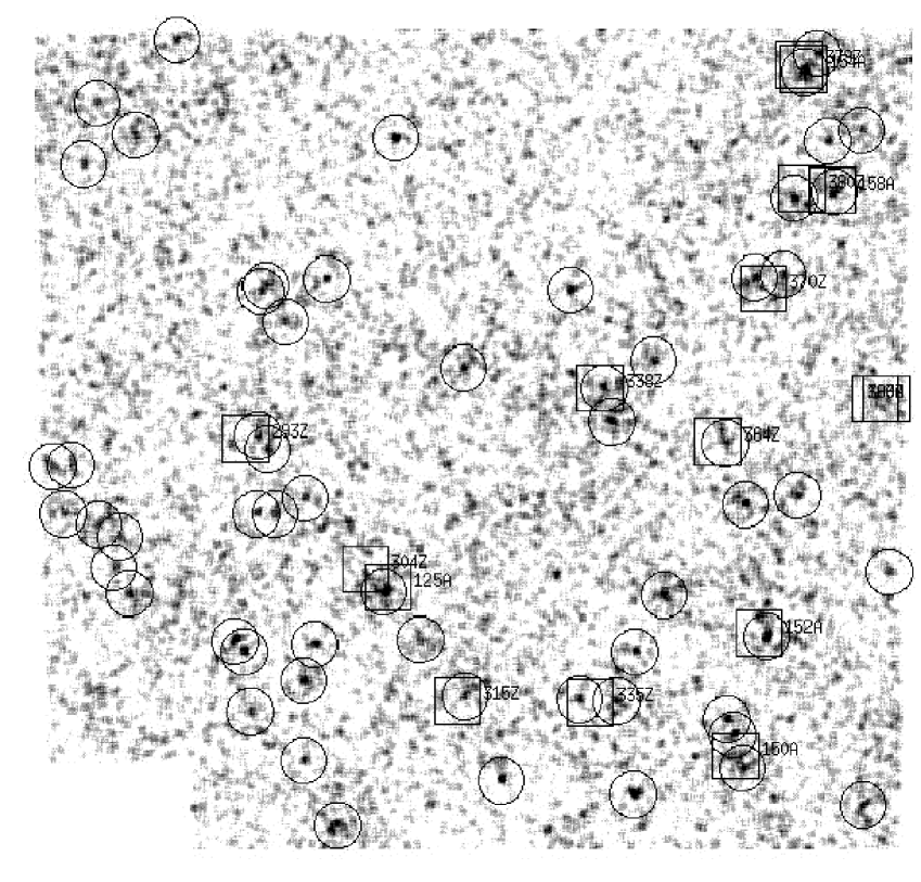
Figure 1: Detected overdensities in the density map in a $5^{\circ}$ x $5^{\circ}$ sky region centered at $RA=1h$ and $Dec=+15^{\circ}$. The smoothing on this map is performed by a 3 x 3 Gaussian filter.
Squares mark known Abell and Zwicky clusters. Circles mark putative - previously unknown - clusters.

In order to exploit the scientific potential of the DPOSS, we developed a model independent procedure to search for cluster candidates. The procedure is detailed elsewhere and therefore we briefly summarize its main characteristics here (Puddu et al. (2000); Puddu et al., in preparation). First, for a given region of the sky, we extract the individual catalogs obtained from the corresponding J, F and N DPOSS plates and calibrate them to the g, r and i Gunn-Thuan System using the procedure described in Weir et al. (1995). Then, after correcting for misclassified objects in at least one of the three filters (see Puddu et al. (2000)), we produce a matched (in the three bands) catalog complete to r $\sim 19.75$ and g $\sim 20.2$ and, in order to ensure completeness, we disregard all objects fainter then r $=19.5$. The spatial galaxy distribution in the matched catalog is then binned into equal area square bins of $1.2$ $arcmin$ to produce a density map. S-Extractor (Bertin & Arnouts (1996)) is run on the resulting image in order to identify and extract all the overdensities having number density $2$ $\sigma$ above the mean background and covering a minimum detection area of $4$ pixels (equivalent to $4.8$ $arcmin^{2}$) on the map convolved with a 3 x 3 Gaussian filter. We wish to stress that, as in the Schectman (1985) approach, we are not assuming any a priori cluster model.
The procedure is run on a given plate catalog to produce a preliminary candidate cluster catalog. All previously known Abell and Zwicky clusters are recovered together with many new cluster candidates (Fig. 1 shows, as an example, DPOSS field 610) which need to be confirmed.
The best way to validate cluster finding algorithms would be to apply them to a field for which redshifts are available for a fairly deep magnitude limited sample of galaxies. Since such a sample does not exist, we were obliged to follow an alternative route. It is well known that early-type galaxies are preferentially located in the cores of rich clusters and that they present a small scatter in the color-magnitude diagram (Dressler (1980); Dressler & Gunn (1992); Stanford et al. (1998)). These properties turn the color-magnitude diagram into a powerful tool to disentangle true clusters from overdensities of galaxies caused by random object alignment along the line of sight.
In this paper we use the early type sequences detected in the color-magnitude diagrams obtained from multiband optical photometry to confirm a sample of 12 candidates. These candidate clusters were selected from some fully reduced DPOSS plates available at the time the test was performed. The selection was performed randomly in order to include overdensities covering a wide range of S/N ratios in the detection maps. We also use a sample of 8 X-ray selected clusters at nearby and intermediate redshift as templates to calibrate the photometric redshift estimate.

The paper is structured as follows: in section 2 we describe the data and the data reduction strategy, in section 3 we show the color-magnitude diagrams for the calibration sample and illustrate the procedure implemented to derive the photometric redshift estimate, while in section 4 we apply this method to the candidates. In section 5 conclusions and future developments are discussed.

Table 1: Selected overdensities.
Notes:(1) Zwicky cluster

OBJ	RA(2000)	Dec(2000)	Richness within	Detection
			the isopleth	S/N
27_694(1)	05 00 07.24	+10 15 52.00	76	8
44_778	08 59 52.68	+04 10 53.20	21	4
17_778	09 08 28.20	+06 03 39.55	63	8
5_778	09 12 11.09	+02 23 10.22	17	4
1_778	09 12 15.34	+02 32 18.11	48	7
64_781	09 57 25.10	+03 39 06.70	27	5
72_781	09 57 53.23	+03 27 10.09	59	7
6_725	15 24 52.60	+11 20 27.10	146	12
1_799(1)	16 03 11.78	+03 14 17.63	132	11
24_694	05 03 38.92	+10 38 08.59	50	7
21_694	05 04 42.34	+10 48 49.00	70	8
26_727	15 57 48.70	+08 52 04.39	8	3

Table 2: Sample of known clusters.
G&L: Gioia & Luppino, 1994; S&R: Struble & Rood, 1999.

Id	RA(J2000)	Dec(J2000)	z	Ref.(z)
MS0821.5+0337	08 24 07.104	+03 27 45.22	0.347	G&L
Abell 1437	12 00 24.960	+03 20 56.40	0.1339	S&R
MS1253.9+0456	12 56 28.827	+04 40 01.87	0.23	G&L
Abell 1835	14 01 02.399	+02 52 55.20	0.2532	S&R
MS1401.9+0437	14 04 29.378	+04 23 00.33	0.23	G&L
MS1426.4+0158	14 28 58.768	+01 45 11.94	0.32	G&L
Abell 2033	15 11 23.518	+06 19 08.40	0.0818	S&R
MS1532.5+0130	15 35 02.739	+01 20 57.15	0.49	G&L

2 Observations and Data Reduction

2.1 The observations and the sample

All data used in this paper were obtained in imaging mode with DFOSC at the ESO 1.54m Danish telescope (La Silla - Chile) during two observing runs (March 1999 and March 2000) blessed by dark time and photometric conditions. The CCD (LORAL/LESSER C1 W7) has 2052 x 2052 pixels, each pixel covering $0.39^{\prime\prime}$, corresponding to a field of $\sim$ $13.3^{\prime}$ x $13.3^{\prime}$. Data were taken in the g, r and i filters of the Thuan & Gunn system (Thuan & Gunn (1976); Wade, Hoessel & Elias (1979)). Seeing averaged $\sim 1.2^{\prime\prime}$ and was always better than $1.5^{\prime\prime}$. The slight difference between our setup and the original Thuan & Gunn filters resulted in a significant color correction which had to be taken into account in the calibration procedure.
Exposure times ranged from 40 to 50 minutes in the g band and 20 to 30 minutes in the r and i bands, depending on the target. In order to obtain higher S/N and more accurate photometric measurements, exposures for those clusters at intermediate redshift were usually repeated in two or three slightly offset frames.
The observed fields (all located in a region with $0^{\circ}<\delta<+12^{\circ}$ and therefore observable from both hemispheres) included 12 candidate clusters plus 8 clusters with known redshifts to be used as comparison sample. In order to use the same material to both calibrate the corresponding DPOSS fields and to validate our algorithm, we selected galaxy overdensities in such a way that we had at least two (up to four) candidates and/or clusters in each DPOSS field. One candidate, observed on two different nights, also provided an independent check of the photometric accuracy of the second run. For the comparison sample we selected 8 clusters from the X-ray selected sample of Gioia & Luppino (1994) and Ebeling et al. (1996).
The equatorial coordinates of the observed fields are given in Tables 1 and Tables 2.
We wish to stress that one of the main problems encountered in our work was the well known lack of a suitable set of photometric standards for the Gunn-Thuan system which, along with the lack of faint stars suitable for CCD observations, very often prevents good coverage of the airmass-color plane. The problem is even worse for observers in the Southern hemisphere where the number of available standards is uncomfortably small. We succeeded, however, in observing an average of 4-5 standard stars per observing night.

2.2 Data Reduction and Photometric Calibration

The raw images (both scientific and calibration) were prereduced using the standard procedures available in the IRAF package. First, the frames were corrected for instrumental effects (overscan and bias) and flat fielded. Individual dome and sky flats in each filter were median stacked to increase the S/N ratio. For the first run, flatfielding was performed using sky flats only, but the experience gained in this run suggested a slightly different procedure for the second run, using dome flats to achieve better correction of the small scale pixel-to-pixel variations. Dome flats were first used to correct the sky flat frames for the higher frequency fluctuations, and the resulting frames were then smoothed and stacked to map the lower frequency fluctuations and combined with the average dome flat to produce the final master flats.
In the first run, we divided the exposures into two or three frames for the same field; in these cases, the images were combined in each filter by medianing (three exposures) or averaging (two exposures) the aligned frames. Standard star photometry was performed using the apphot package in IRAF. Due to the need to defocus most of the stars to avoid saturation, stars were measured through 10 apertures with diameters up to $90$ pixels ($35.1^{\prime\prime}$), and the local sky was determined using a $10$ pixel wide annulus outside of the largest aperture. In order to determine the zero-point offset and the airmass and color terms we used the $40$ pixels ($\simeq 15^{\prime\prime}$) aperture, for the focused and unsaturated stars, and the asymptotic magnitudes for the defocused ones.

The IRAF fitparams task was used to fit the data with the relation

$${m_{true}=m_{inst}+Z_{p}+K_{e}\cdot X+CI\cdot color_{inst}}$$ (1)

where $Z_{p}$ is the zero point of the magnitude scale; $K_{e}$ is the extinction coefficient and $X$ the airmass; $CI$ is the instrumental color term coefficient. For the first run (March 1999), due to the paucity of standard stars, we could determine single night coefficients only for the r and i filters. The coefficients were consistent from one night to the other and we used a mean fit for the g-r color.
For the second run (March 2000) we instead derived the coefficients for each night and in each band (using the g-r and r-i colors). The resulting calibration coefficients of the various nights are consistent within the errors and, therefore, in order to improve the quality of the fit, we adopted a unique pair of extinction coefficient and color term for the whole run. These constants were then used to derive the zero points for each night. In Fig. 2 we show for the g and r filters, the fit residuals as a function of the estimated magnitude, using different symbols for different nights.

Figure 2: Residuals for the g (upper panel) and r (lower panel) fit. Different symbols refer to different nights. The outlier point is Ross 683, which turns out to be consistently brighter than expected in all four observed nights.

Figure 3: Comparison between the photometry of the candidate cluster 64_781 between nights 2 and 4: the plot shows the g or r magnitude offset vs. the g or r magnitude

Figure 4: Color - color diagram for the Gunn & Thuan standards (open circles) and for a sample of stars (filled symbols) extracted from the field 5_778.

2.3 Object Detection and Photometry

The object catalogs were produced individually for each band using S-Extractor: all objects larger than $4$ pixels and $2\sigma$ above the background counts were included and their photometric and morphological features measured. We used a photometric reference aperture with a diameter $\sim 3$ times larger than the average seeing.
For each CCD field, the three single band catalogs where matched taking into account the shifts between pointings (measured using the geomap and geotrans IRAF tasks).

To obtain an estimate of the external photometric errors, the candidate cluster 64_781 was observed on two different nights. In this way we could evaluate possible night-to-night magnitude offsets in both the g and r filters. The typical weighted mean values for these offsets are $0.05$ for the g filter and $0.007$ for the r filter, i.e. they are of the same order as the rms errors from the three parameter calibration fit (Fig. 3).

Since our goals require high accuracy for the color determination, we further checked the photometric calibration, using the following test: in the color-color diagram (Fig. 4) we plotted the linear sequence of the Gunn-Thuan standards (open circles) together with all the unsaturated stars (S-Extractor stellarity index $<0.8$) within the limiting magnitude, selected from some CCD cluster candidate fields (in Fig. 4 we show the 5_778 field). For all of these fields, the sequence of the selected stars is linear (excluding the very red sources, dominated by stars of spectral type M, which have a constant g-r color while r-i depends on the spectral subtype; see Fukugita et al. (1996) and Finlator et al. (2000)) and overlap quite well with the standard sequence. This means that the colors of the main sequence stars are well determined, since the relation between g-r and r-i is the same for the cluster field stars and for the standards.

3 Validation method via color-magnitude diagrams

From the g and r matched catalogs we excluded obvious stars (stellarity index $>0.95$) and then selected a box of $\sim 300$ pixels in size (corresponding to a typical core cluster diameter of $\sim 750$ kpc at $z\sim 0.2$), centered on the approximate cluster center and a second box of equal size located as far as possible from the cluster, to be used for the evaluation of the background contribution.

Our procedure is summarized in Fig. 5, which shows the results for four sample candidates which are representative of the various morphologies encountered.
For all candidates in our sample we first obtained the color-magnitude diagrams for both the cluster and background objects. Then, in order to enhance the early-type sequence, we performed the statistical subtraction of the background contribution by eliminating for each object in the background diagram the corresponding nearest galaxy in the cluster+background diagram. If we then isolate the objects contained within a narrow strip of the color-magnitude diagram centered around the early-type sequence, the galaxy overdensities become more evident in both the spatial distribution and in the number counts radial profile (Fig. 5; the radial profile was calculated by choosing as cluster center the barycenter of the density distribution).
The plots in Fig. 5 can be used as a criterion to distinguish true clusters (candidates (a) and (b)), even if they are difficult to detect. In some cases (usually candidates which are either too distant or too poor), despite the presence of an apparent sequence in the color-magnitude diagram, the objects do not form a physical overdensity, but turn out to be uniformly distributed on the sky. In these cases it is more difficult to reach any definite conclusion about the physical nature of the candidate.

3.1 Color-magnitude diagrams for the calibration cluster sample

We chose as templates a sample of X-ray clusters for which, at least in principle, the early-type sequence in the color-magnitude diagrams should be easily detectable. This sample was also used to investigate whether or not it was possible to derive an acceptable estimate of the redshift from the g-r color of the early-type sequences.

In Fig. 6 we plot the color-magnitude diagrams for the 8 clusters in the X-ray sample including only the cluster contribution (i.e., after the statistical subtraction of the background). It is quite evident that some of the early-type sequences are only broadly outlined (MS1401, MS1426, MS1532), which may be caused either by the intrinsic faintness of the cluster members or by cluster structural features (poorness, looseness and presence of interacting systems; see the comments in Gioia & Luppino (1994) about these three clusters). For each cluster we derived a median g-r color using only the 5 brightest galaxies after the background subtraction (continuous line), from which we also estimated the redshift. The crosses represent the g-r colors corresponding to the literature redshifts.

3.2 Photometric Redshift Estimate

Some techniques for deriving redshifts from broadband photometry consist of matching observed elliptical galaxy colors with those predicted from the Spectral Energy Distributions (SEDs) (Visvanathan & Sandage (1977)) of a template elliptical galaxy at zero-redshift and corrected according to the redshift: since ellipticals become redder as their redshift increases and since the redshift dependent correction (k-correction), is monotonically increasing in the near and intermediate redshift Universe, colors can be used to infer the cluster redshift.
There is no agreement in the literature for the g-r color of ellipticals at zero-redshift: $0.47^{m}$, according to Schneider, Gunn & Hoessel (1983); $0.38$ mag for Frei & Gunn (1994); $0.40^{m}$ to $0.49^{m}$ according to Fukugita et al. (1995). Differences in these values likely depend on the galaxy spectrum template adopted for the ellipticals and on the use of a synthetic or an observed spectrum for the standard stars defining the photometric system. To a lesser extent, differences are due to the variations in the actual shape of the Gunn g and r filters (convolved with the atmosphere, mirror and glass transmissions, CCD quantum efficiency, etc.) and possibly also to the way in which the colors are computed.

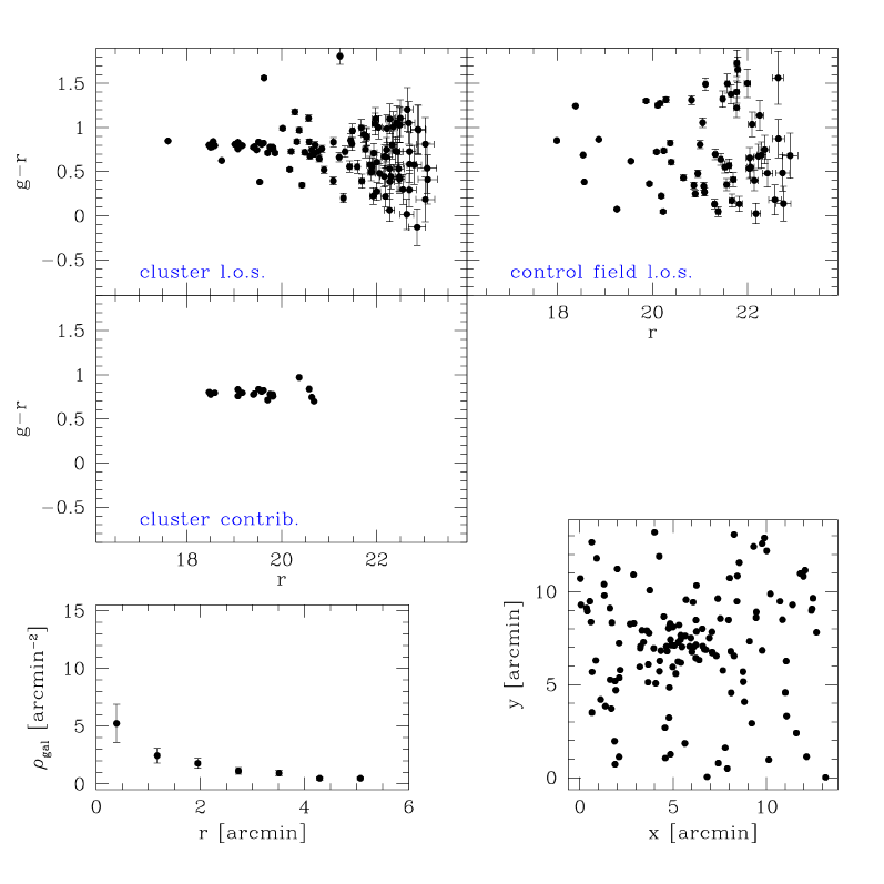
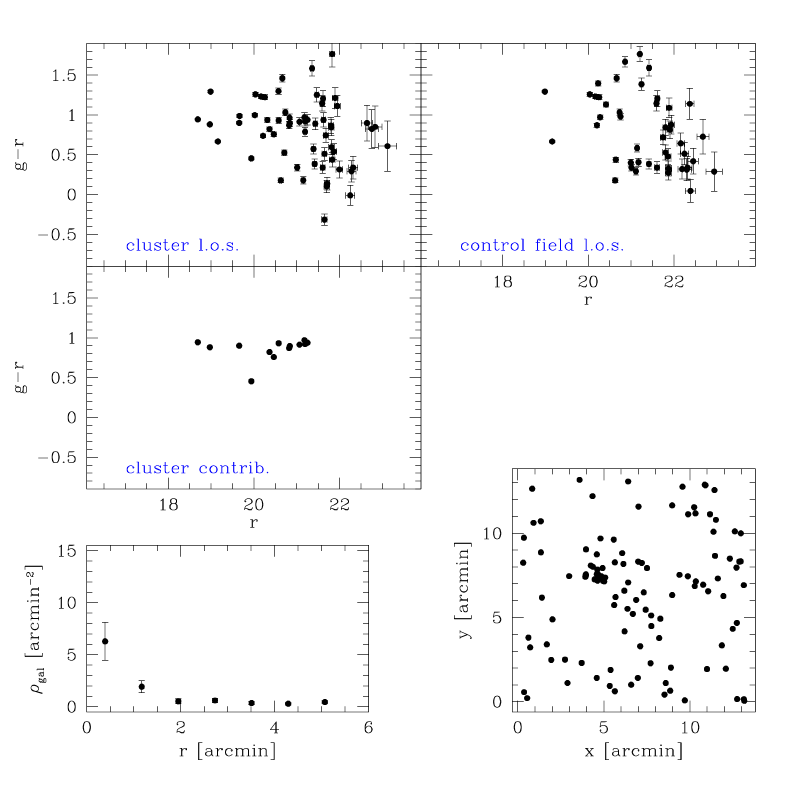
(a)                                                                       (b)

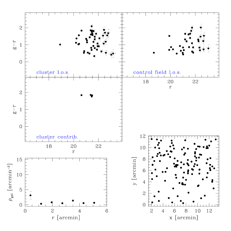
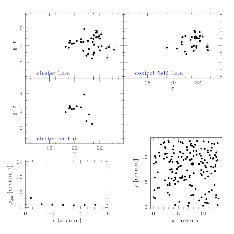
(c)                                                                       (d)

Figure 5: Complete set of plots for two confirmed (upper half) and two uncertain (lower half) cluster candidates. Each set of plots consists of color-magnitude diagrams for background + cluster box; color-magnitude diagrams for background box; color-magnitude diagrams for statistically corrected cluster objects; radial profiles and spatial distributions over the CCD field of the objects within a color strip around the early-type sequence. The four sets of plots refer respectively to: (a) OV17_778, a typical rich nearby cluster (z$\sim$ 0.2); (b) OV6_725, a poor cluster at redshift z$\sim$ 0.2; (c) OV21_694 and (d) OV24_694, uncertain clusters, with less evidence for the early-type sequence in the color-magnitude diagrams, and for density peaks in the spatial distribution.

Figure 6: Color-magnitude diagrams after statistical background subtraction for the X-ray cluster sample. According to Gioia & Luppino (1994), MS1401 is a loose cluster, without a dominant galaxy; MS1426 contains spirals and possibly interacting systems, and moreover may be two clusters in projection. A Seyfert galaxy at z=0.074 is present in the foreground of the MS1532 field. Abell 2033 is of Bautz-Morgan type III and richness class 0.

In the absence of a definite value, we left the zero-redshift color of ellipticals as the unique free parameter and constrained it with our own observations by (robustly) fitting the relation between color and redshift. Fig. 7 shows (filled dots) the observed colors from the color-magnitude relation vs. known spectroscopic redshift for our X-ray cluster sample. The expected color of ellipticals (continous line) were computed using the Schneider, Gunn & Hoessel (1983) k-correction curve and our own determination of the elliptical colors. The average g-r color of ellipticals of zero redshift turns out to be $0.44^{m}$, i.e. the average of the four previously quoted literature values. Errors on the colors are given as one third of the interquartile range, which roughly corresponds, for a Gaussian distribution of five points to the error on the mean. We prefer these to the standard error since they are more robustly determined. Figure 7 shows that all points are compatible with the curve within $1\sigma$, excluding two points , which are within $2\sigma$. The agreement is good, provided that there is only one free parameter (the rest-frame elliptical color). Figure 8 compares the photometric redshift, estimated from the color-magnitude diagrams and the spectroscopic redshift. The agreement is good, and the error (interquartile range) on the redshift is, on average, $\delta z=0.01$, i.e. $3000$ km/s. Tab. 3 lists the estimated photometric redshifts, with the errors computed as previously defined, for the putative clusters; since these clusters are fairly rich systems, this error is likely to be a lower limit.

Figure 7: The observed colors from the color-magnitude relation and their errors for the X-ray cluster sample (filled circles) are plotted, compared to the expected color of ellipticals (continuous line) as a function of spectroscopic redshift.

Figure 8: Photometric vs. spectroscopic redshift. The solid line is the bisector and is not derived from data fitting.

4 The validation of the candidate cluster sample

In Fig. 9 we show the early-type sequences obtained (after subtracting the background) for the 12 candidate clusters in our sample. We confirm 9 of the 12 candidates as true clusters, one is a fortuitous detection of a cluster at $z\sim 0.4$, one is a false detection and the last is undecidable on the basis of the available data.

The better definition of the early-type sequences observed in the DPOSS confirmed clusters sample with respect to the X-ray sample is likely due to the different specific properties of the two samples: at a given z, our optically selected clusters are on the average richer and more centrally concentrated then the X-ray selected ones.

For the cluster OV27_694, the early-type sequence is less defined due to the overlap of two independent clusters/groups along the line of sight.
The case of OV21_694 merits special attention. As a visual inspection of the corresponding POSS-II F plate shows, the marginal detection of an early type sequence (Fig. 5 and 9) seems to be due to the chance alignment of a distant cluster (at redshift $z\sim 0.4$) with a rich galaxy field. The existence of such a foreground rich field has therefore triggered the search algorithm. As far as OV24_694 and OV26_727 are concerned, the marginal evidence for an early-type sequence does not correspond to a defined overdensity in the number count radial profiles (using galaxies in the strip centered on the mean g-r color). The case of OV26_727 is a false cluster detection, since it has a low S/N ratio and low isophotal richness (see Tab. 1; it may be a group). Visual inspection of the POSS-II plate shows that OV24_694 lies in a crowded field rich with galaxies; from the sky diagram (Fig. 5, case (d)) it is also evident that a large fraction of these foreground galaxies have the same color. Thus, this field could be part of a larger loose cluster or a cluster in a region with variable background.

Figure 9: Color-magnitude diagrams after statistical background subtraction for the 12 candidate clusters with complete observations. The three upper right diagrams refer to not confirmed candidates (OV21_694, OV24_694, OV26_727).

Table 3: New Redshift Estimate.
(1): the faintness of the galaxies, as observed both on CCD and on plate suggests that the candidate cluster is far, as puts forward by the redness of the color-magnitude relation; (2): the color-magnitude shows a large scatter, suggesting that this cluster is possibly contaminated by a foreground group.

OBJ	z est.	z est. min	z est. max
17_778	0.195	0.169	0.209
1_778	0.234	0.219	0.247
1_799	0.314	0.299	0.326
21_694(1)	0.488	0.466	0.511
24_694	0.282	0.271	0.295
26_727	0.216	0.204	0.23
27_694(2)	0.204	0.183	0.218
44_778	0.243	0.228	0.255
5_778	0.189	0.159	0.205
64_781	0.139	0.110	0.159
6_725	0.218	0.205	0.232
72_781	0.219	0.207	0.234

5 Summary and conclusions

The aim of our work was to test the validity of a model independent cluster finding algorithm, implemented to extract a statistically well defined sample of cluster candidates from photometrically calibrated DPOSS data (see Paper I for details). The advantages of a model independent approach are that i) the program does not assume any a priori knowledge about the clusters, and ii) it objectively looks for statistically meaningful overdensities in the galaxy density field. The main problem in validating any cluster finding algorithm is the lack of a suitable data set to use as a template, i.e., the lack of a region of the sky containing a large sample of clusters with well defined redshifts and properties. In the absence of such a data set, we adopted a photometric approach based on the use of the sequence defined in the color-magnitude diagrams of clusters by bright early-type galaxies as a diagnostic tool. We obtained deep multiband CCD photometry for a sample of 12 candidate clusters extracted from the DPOSS data, plus an additional sample of 8 X-ray clusters with known redshifts to be used as a template to calibrate the photometric redshift procedure. Results may be summarizied as follows: among the 12 clusters candidates, 10 are confirmed clusters, 1 is false and 1 is uncertain. The X-ray selected cluster sample was then used both to check the accuracy ($\Delta z\simeq 0.01$) and to find the zero point (i.e., the average zero-redshift $g-r$ color for elliptical galaxies in our system:$(g-r)_{0}=0.44$) for the photometric redshift procedure. This procedure is being applied to a larger sample of clusters derived from both DPOSS calibration data and from other archive datasets. Future papers will deal with the analysis of a larger sample of clusters ($\sim 200$) identified on both DPOSS and archive data and will focus on the derivation and analysis of luminosity functions (both individual and cumulative) and of radial number count profiles (Strazzullo (2001)).

References

- Abell (1958) Abell, G.O. 1958, A&AS, 3, 211
- Abell et al. (1989) Abell, G.O., Corwin, H.G., Olowin, R.P. 1989, AJSS, 70, 1
- Andreon et al. (1997) Andreon, S., Zaggia, S., de Carvalho, R., et al. 1997, in Rencontres de Moriond, eds. G. Mamon, T. X. Thuan and Y. T. Van, Edition Frontieres (Gif-sur-Yvette).
- Bertin & Arnouts (1996) Bertin, E. & Arnouts, S. 1996, AASS, 117, 393
- Couch et al. (1991) Couch, W.H., Ellis, R.S., Malin, D.F., et al. 1991, MNRAS, 249, 606
- Dalton et al. (1992) Dalton, G.B., Efststhiou, G., Maddox, S.J., et al. 1992, ApJ, 390, L1-L4
- (7) Djorgovski, S.G., de Carvalho, R.R., Gal, R.R., et al. 1998, in IAU Symp. 179, McLean, B.J., Golombeck, D.A., Hayes, J.J.E., Payne, H.E. eds., Kluwer Academic Publ., p. 424
- (8) Djorgovski, S.G., Gal, R.R., Odewahn, S.C., et al. 1998, in Wide Field Surveys in Cosmology, S. Colombi, Y. Mellier, and B. Raban, Gif sur Yvette eds., Eds. Frontières, p. 89
- Dodd & MacGillivray (1986) Dodd, R.J., MacGillivray, H.T. 1986, AJ, 92, 706
- Dressler (1980) Dressler, A. 1980, ApJ, 236, 351
- Dressler & Gunn (1992) Dressler, A. & Gunn, J.E. 1992, ApJS, 78, 1
- Ebeling et al. (1996) Ebeling, H., Voges, W., Bohringer, H., et al. 1996, MNRAS, 283, 1103
- Finlator et al. (2000) Finlator, K., Ivezic, Z., Fan, X., et al. 2000, AJ, 120, 2615
- Frei & Gunn (1994) Frei, Z., Gunn, J.E. 1994, AJ, 108, 1476
- Fukugita et al. (1995) Fukugita, M., Shimasaku, K.,Ichikawa, T. 1995 PASP, 107, 945
- Fukugita et al. (1996) Fukugita, M., Ichikawa, T., Gunn, J.E., et al. 1996 AJ, 111, 1748
- Gal et al. (1998) Gal, R.R., de Carvalho, R.R., Djorgovski, S.G., et al. 1998, American Astronomical Society Meeting, 193, 202
- Gal et al. (1999) Gal, R.R., Odewahn, S.C., Djorgovski, S.G., et al. 1999, in Photometric Redshifts and Detection of High Redshift Galaxies, ASP Conference Series, vol. 191, Eds. Ray Weymann et al., p. 185
- (19) Gal, R.R., de Carvalho, R.R., Odewahn, S.C., et al. 2000 AJ, 119, 12
- (20) Gal, R.R., de Carvalho, R.R., Brunner, R., et al. 2000 AJ, 120, 540
- Gioia & Luppino (1994) Gioia I.M. & Luppino G.A. 1994, AJS, 94, 5838
- Kepner et al. (1999) Kepner, J., Fan, X., Bahcall, N., et al. 1999 ApJ, 517, 78
- Kim et al. (2000) Kim, R., Strauss, M., Bahcall, N., et al. 2000, in Clustering at High Redshift, ASP Conference Series, Vol. 200, p.422 Edited by A. Mazure, O. Le Fevre, and V. Le Brun.
- Lumsen et al. (1992) Lumsden, S.L., Nichol, R.C., Collins, C.A., et al. 1992, MNRAS, 258, 1
- Olsen et al. (1999) Olsen, L.F., Scodeggio, M., da Costa, L., et al. 1999, A&A, 345, 6810
- Postman et al. (1986) Postman, M., Geller, M.J., Huchra, J.P. 1986, AJ, 91, 1267
- Postman et al. (1996) Postman, M., Lubin, L.M., Gunn, J.E., et al. 1996, AJ, 111, 615
- Puddu et al. (2000) Puddu, E., Andreon, S., Longo, G., et al. 2000, MmSAI, vol. 71, n.4, in press
- Schectman (1985) Schectman, S.A. 1985, AJS, 57, 77
- Schneider, Gunn & Hoessel (1983) Schneider, D.P., Gunn, J.E., Hoessel, J. 1983, ApJ, 264, 337
- Stanford et al. (1998) Stanford, S.A., Eisenhardt, P.R. & Dickinson, M. 1998, 1998, ApJ, 492, 461
- Strazzullo (2001) Strazzullo, V., Master Thesis, in preparation
- Struble & Rood (1999) Struble, M.F. & Rood, H.J. 1999, ApJS, 125, 35
- Sutherland (1988) Sutherland, W. 1988, MNRAS, 234, 159
- Thuan & Gunn (1976) Thuan, T.X. & Gunn, J.E. 1976, PASP, 88, 543
- Visvanathan & Sandage (1977) Visvanathan, N. & Sandage, A. 1977, ApJ, 216, 214
- Wade, Hoessel & Elias (1979) Wade, R.A., Hoessel, J.G., Elias, J.H. et al. 1979, PASP, 91, 35
- Weir, Djorgovski & Fayyad (1995) Weir, N., Djorgovski, S.G., Fayyad, U.M. 1995, AJ, 110, 1
- Weir et al. (1995) Weir, N., Fayyad, U.M., Djorgovski, S.G., Roden, J. 1995, PASP, 107, 1243
- Zwicky et al. 1961- (68) Zwicky, F., Herzog, E., Wild, P., et al. 1961-68, Catalogue of Galaxies & Clusters of Galaxies.