Revisiting Brightest Cluster Galaxy Evolution with the Las Campanas Distant Cluster Survey

Abstract

We investigate the influence of environment on brightest cluster galaxy (BCG) evolution using a sample of 63 clusters at 0.3 $\leq z\leq$ 0.9 drawn primarily from the Las Campanas Distant Cluster Survey and follow-up $V$, $I$, and $K^{\prime}$ photometry. The luminosity evolution of the entire BCG sample is not adequately described by a single evolutionary model. Using the integrated light from the cluster detection as a proxy for cluster L_x and the suggestion by Burke, Collins, & Mann, we set L${}_{x}=2\times 10^{44}$ ergs s^-1 to be the division between high and low luminosity clusters. At high redshift ($z>0.6$) BCGs from low-L_x clusters are fainter, on average, than those from high-L_x clusters and are best modeled as having constant luminosity with redshift. The BCGs from high-L_x cluster are best modeled as having a stellar population that formed at large redshift ($z_{form}>5$) and is passively evolving. However, for the entire BCG population, the observed $V-I$ and $I-$$K^{\prime}$ colors are well described by a single evolutionary model in which the stellar populations have $z_{form}>5$ and subsequently passively evolve. We conclude that accretion is proportionally more significant for BCGs in lower mass clusters at these redshifts (factor of 2 to 4 increase in mass since $z\sim 1$ for the low L_x systems; Aragon-Salamanca et al. ) and that the accreted matter is in the form of systems with evolved stellar populations.

1. Introduction

In standard hierarchical formation scenarios, structure formation occurs first in regions of highest overdensity. As a result of this accelerated formation, it is generally believed, for example, that cluster galaxies are on average older than field galaxies. However, studies comparing the evolution of galaxies in different environments are difficult because identifying equivalent field and cluster populations is an ill-defined problem and because the effects of various physical processes (interactions, ram pressure stripping, tidally triggered star formation, harassment by the global cluster potential, etc.) are poorly understood. Selection by morphology, luminosity, color, environment, or any other observable property of galaxies has the potential to bias the sample.

One galaxy population that can be unambiguously identified in a variety of environments, by definition, is the dominant galaxy, referred to as the brightest cluster galaxy (BCG) in clusters and the brightest group galaxy (BGG) in groups. Although the particular galaxy that is the BCG or BGG may change with time in any environment, that process is part of the evolution one aims to study and the sample definition is relatively unambiguous and well-suited for comparison to simulations. Over the last 50 years, many have studied the properties of BCGs from redshifts 0 to $\sim$ 1 (some highlights include Humason, Mayall, & Sandage 1956; Sandage, Kristian, & Westphall 1976; Hoessel 1980; Schombert 1986; Graham et al. 1996); initially with the intent to use BCGs as standard candles, later to study galaxy evolution. We revisit the topic of BCG evolution in light of recent claims of significant accretion (Aragon-Salamanca, Baugh, & Kauffmann 1998; hereafter ABK) and environmentally induced differences (Burke, Collins, & Mann 2000; hereafter BCM) using a large sample of BCGs drawn from the Las Campanas Distant Cluster Survey (LCDCS; Gonzalez et al. 2001a). Although BCG evolution may be quite distinct from galaxy evolution in general, its study may shed light on the process of hierarchical structure formation in dense environments.

BCGs are the most massive and luminous galaxies. However, the findings that at least some BCGs are not drawn from the luminosity function of cluster ellipticals (Tremaine & Richstone 1977; Dressler 1978) and that BCGs may have different luminosity profiles than other giant ellipticals (Oemler 1976; Schombert 1986) suggest that they have a different evolutionary history than standard cluster ellipticals. Aragon-Salamanca et al. (1993; hereafter A93) observed BCGs at high redshift ($0.5<z<0.9$) in the $K$-band and found that while the BCG colors agree with the prediction of passive evolution models with high formation redshifts ($z_{form}\gtrsim 2$), similar to the results for cluster ellipticals (Bower, Lucey, & Ellis 1992), their luminosities match the prediction of no-evolution models. Because stellar populations dim as they age, ABK interpret this lack of even passive luminosity evolution to imply significant, relatively recent mass accretion by the BCGs. Parameterizing the necessary mass accretion, ABK estimate that BCGs have grown by a factor of two to four in mass since $z\sim 1$, a result which they find to be consistent with the expectation from hierarchical models as described by semi-analytic models of galaxy evolution (cf. Kauffmann, White & Guiderdoni 1993)

This rather attractive agreement between observations and simulations for the evolution of BCGs over $\sim$ 75% of the age of the Universe has recently been questioned. The focus of the current discussion is whether all BCGs are similar, and in particular whether environment plays a critical role in determining the properties of BCGs (Hudson & Ebeling 1997; Collins & Mann 1998, hereafter CM; and BCM). BCM study the BCGs of 76 x-ray selected clusters in the $K$-band and find that BCGs from low-L_x clusters (L${}_{x}<2.3\times 10^{44}$ ergs s^-1) display no luminosity evolution. (We will refer to the BCGs from high and low L_x clusters as high-L_x and low-L_x BCGs.) Furthermore, they find that the ABK sample primarily consists of low-L_x BCGs at $z>0.5$. Therefore, the BCM observation of no luminosity evolution in the BCGs from low-L_x clusters is entirely consistent with that of ABK. However, they find that the luminosities of high-L_x BCGs have evolved since $z\sim 1$. The stellar populations of their high-L_x BCGs are consistent with the luminosity predictions of passive evolution models with a high formation redshift ($z_{form}\gtrsim 5$). Because high-L_x clusters best match the cluster selection adopted for comparison to the semi-analytic models, they reinvestigate the parameterization of the mass evolution of high-L_x BCGs and find substantially lower rates of mass accretion, at most a factor of $\sim$2 increase in mass since $z\sim 1$. This result suggests that BCGs from high-L_x clusters experience a different evolutionary scenario than those from low-L_x clusters.

Because BCG properties appear to depend upon properties of the host cluster, it is imperative that samples are drawn from large surveys that span as wide a range of cluster properties as possible to probe that dependence, and that the samples are sufficiently large to average over outliers. Both ABK and BCM have relatively small samples at $z>0.5$ ($\sim$a dozen each) that are biased with respect to cluster L_x (ABK toward low-L_x systems and BCM toward high-L_x systems). Obviously, enlarging the samples of these high redshift clusters has been difficult and any potential advance should be exploited. We examine the evolutionary history of BCGs using a new sample of high redshift clusters drawn primarily from the LCDCS (Gonzalez et al. 2001a).

The LCDCS is a drift scan survey, conducted by the authors at the Las Campanas Observatory in 1995, that covers 130 deg² of the southern sky and yielded over 1000 cluster candidates. Rather than selecting overdensities of resolved galaxies, our cluster-finding technique relies upon the assumption that the total light from a distant cluster is dominated by the contribution from unresolved sources. In an intrinsically uniform image, the integrated diffuse cluster light will manifest itself as a low surface brightness enhancement. Not only does this catalog result in a factor of 5 increase in the number of cataloged clusters at these redshifts, but because our cluster identification criteria differs from those utilized in previous surveys, this catalog provides an independent, well-defined sample with which to compare the results from more traditional surveys. Details of the survey and the catalog of clusters can be found in Gonzalez et al. (2001a).

Because extensive follow-up observations are prohibitively time-intensive, the BCGs we examine here are a small subset of the final catalog. We use 54 clusters from the LCDCS and 9 northern clusters from a smaller Palomar 5m survey (for which the data was originally taken as part of the Palomar Transit Grism Survey for high redshift quasars; Schneider et al. 1994 and analyzed in Dalcanton 1995) which we originally utilized to test the low surface brightness technique. The combined sample consists of 63 clusters, 17 of which are spectroscopically confirmed and 46 of which have photometrically estimated redshifts (Nelson et al. 2001a). We obtain deep follow-up imaging in $V$, $I$, and $K^{\prime}$ , although not every BCG is imaged in every band. In §2 we describe the data. We include a brief description of the survey, cluster candidate selection and classification in §2.1. In §2.2 we describe follow-up observations and photometry. Next, we give a summary of our photometric redshift estimators and BCG selection in §2.3 and §2.4, respectively. In §2.5 we describe the technique used to estimate L_x. In §3 we examine the evolution of BCGs in both luminosity and color. Finally, we summarize our results and conclusions in §4.

2. The Data

Our data originate from a variety of telescopes and instruments. We identify the candidate galaxy clusters using drift scans and techniques described briefly below for context, but in full detail by Gonzalez et al. (2001a). The cluster sample and observations used here stem from deep optical and infrared follow-up imaging of a small subset of the full catalog which was obtained to aid in the classification of candidates and to develop photometric redshift indicators. We will briefly review the classification criteria based upon the deep imaging and our photometric redshift estimators. Nelson et al. (2001a) contains a full description.

2.1. Cluster Sample

We draw our clusters from two optical drift scan surveys. The first is a $\sim 17.5$ deg² Palomar 5m survey using the 4-shooter camera (Gunn et al. 1987) and the F555W “wide $V$” filter (Dalcanton et al. 1995, 1997). Dalcanton et al. (1995, 1997) made use of existing scans (originally taken as part of the Palomar Transit Grism Survey for high redshift quasars; Schneider et al. 1994) to verify the low surface brightness (LSB) technique for detecting LSB objects to the required central surface brightness. This survey identified more than 50 northern hemisphere cluster candidates. The second is a 130 deg² survey of the southern sky conducted at the Las Campanas Observatory 1m telescope over 10 nights by the authors using the Great Circle Camera (Zaritsky, Shectman, & Bredthauer 1996) and a wide filter, denoted as $W$, that covers wavelengths from 4500 Å to 7500 Å. This survey was specifically designed to study LSB galaxies and high redshift galaxy clusters. We stagger scans in declination by half of the field-of-view (24 arcmin) so that each section in the survey is observed twice, each time with a different region of the detector. The sidereal rate limits exposure times to $\sim$97 sec per scan at the declination of the survey ($-10^{\circ}$ to $-12^{\circ}$), so that the net exposure time is $\sim$195 sec at any location. The pixel scale is 0.7 arcsec/pixel with a typical seeing of about 1.25 arcsec. The full region surveyed measures $\sim 85^{\circ}\times 1.5^{\circ}$ and is embedded within the area covered by the LCRS (Shectman et al. 1996). The result of iterative flatfielding, masking, filtering, and object detection is a catalog of $\sim$ 1000 cluster candidates (Gonzalez et al. 2001a provide a full description of the method and catalog) with an estimated 30% contamination rate.

From the drift scans, we select a set of candidates for which to obtain deep follow-up imaging in $V$, $I$, and $K^{\prime}$ . These deeper images allow us to classify detections and train the cluster-finding algorithm. The cluster candidates presented in this work were confirmed as clusters based upon the following criteria: 1) the appearance of the background-subtracted $I-$band luminosity function, in particular a well populated and defined bright end of the luminosity function; 2) the presence of a prominent red envelope in the $V-I$ CM diagrams, and 3) a well-defined concentration in the surface density of galaxies, in particular a high degree of spatial clustering of red galaxies. A cluster candidate that strongly satisfies any of these three criteria is considered a viable cluster. We do not require successful candidates to satisfy all three criteria for two reasons. First, we do not have the necessary data to evaluate every cluster equivalently. Second, we have confirmed clusters that do not strongly satisfy all three criteria (for example, high redshift clusters generally have less prominent red envelopes due to the combination of cosmological shifting of light out of the $V$-band and our modest exposure times; Nelson et al. 2001a). We acknowledge that our classification procedure is subjective, but simulations demonstrate that random fields and non-cluster detections (LSBs and spurious detections) do not yield well-defined luminosity functions nor prominent red envelopes (Nelson et al. 2001a). Nevertheless, we will discuss the effect of significant contamination on our results in §3.1.1.

Because the original goal of the follow-up imaging was to test our cluster selection algorithms, the cluster subsample is heterogeneous and thus includes both some of our best and some of our worst candidates. In addition, since our selection procedure evolved during this testing process, some of the confirmed candidates presented here are not in the final, statistical cluster catalog presented by Gonzalez et al. (2001a). We expect no particular biases in BCG properties from this procedure, except those that correlate with cluster properties. The potentially influential cluster properties include concentration and cluster mass, which factor into the cluster selection and which are present at some level in all cluster surveys. These biases are discussed in detail in §2.4.

2.2. Optical and Infrared Photometry

We briefly review the data acquisition and reduction process. Readers interested in a more detailed description are referred to Nelson et al. (2001a). We image our clusters in the Johnson $V$ and Cousins $I$-band because these bands straddle the Ca II H & K break for galaxies at redshifts $0.3\leq z\leq 0.9$, and $K^{\prime}$ because it probes the older, quiescent stellar populations. Because the majority of our photometry was completed before the cluster finding algorithm was fine-tuned (indeed it was necessary to help train the algorithm), we imaged some candidates only in $I$, to provide more images of potential clusters at the expense of color information. The data were collected at a variety of telescopes from 1996 to 1998. Northern clusters were generally imaged at the Palomar 1.5 m telescope and the Lick 3 m telescope, while southern clusters were generally imaged at the Las Campanas Observatory using the 1 m and 2.5 m telescopes. Both the optical and infrared data were reduced following standard procedures (see Nelson et al. 2001a for details). We calibrated the optical data using Landolt’s standard fields (Landolt 1983, 1992). The $K^{\prime}$ -band data was calibrated using the HST faint near-IR standards (Persson et al. 1998).

Table 1 contains information regarding the observations of each cluster. The first column lists the cluster designation. RA and DEC (2000.0) are in the next column, where the center of the cluster is taken to coincide with the centroid of the low surface brightness fluctuation. The last six columns contain the exposure time and seeing for each of the three photometric bands, $V$, $I$, and $K^{\prime}$ . In summary, 97$\%$ of our clusters are imaged in $I$, $54\%$ in $V$, $35\%$ have infrared $K^{\prime}$ data, and $29\%$ have spectroscopy. Some clusters were imaged twice in various photometric bands and are listed twice in Table 1. If one data set is clearly of superior quality than the other, we use the superior data. Otherwise we average the photometric results.

The correlation between the luminosity of the BCG measured within the fixed radius $r_{m}$, referred to as the metric aperture or L_m, and the logarithmic slope of the BCG curve of growth, $\alpha\equiv[$d log(L${}_{m})/$d log$(r)]|_{r=r_{m}}$ (Hoessel 1980; Lauer & Postman 1994; Postman & Lauer 1995, hereafter PL95; Hudson & Ebeling 1997; CM) is often used to place BCG luminosities on a standard-candle scale. Such an adjustment typically reduces the scatter in the distance-magnitude relation by $\sim 0.1-0.2$ mag. Consequently, BCG photometry is predominantly measured using a fixed aperture of projected physical radius ($\sim$10 kpc locally, and $\sim$25 kpc at high redshift). However, we choose neither to measure our BCG photometry with fixed metric apertures, nor to correct their luminosities using the L${}_{m}-\alpha$ relation, for two reasons. First, seeing corrections that must be applied to fixed aperture magnitudes are too uncertain (especially at high redshift, because the seeing varied dramatically from run to run, 0.8${}^{\prime\prime}-3^{\prime\prime}$ in the optical and 0.6${}^{\prime\prime}-2^{\prime\prime}$ in the infrared). Second, as we describe in detail below, the majority of clusters in our sample do not have spectroscopic redshifts. Instead we rely upon photometric redshift estimators whose associated errors ($\sigma_{phot}\sim 0.06$) are comparable to the L${}_{m}-\alpha$ correction. Applying the L${}_{m}-\alpha$ relation to BCG photometry typically changes M_BCG by $\sim$0.5 mag (see Figure 1 in PL95; Figure 10 in CM). For the redshift range in which the bulk of our clusters lie, the uncertainty in $z_{phot}$ corresponds to $\Delta M_{bcg}\sim$0.2-0.4. Despite the potential increase in scatter by not using the L${}_{m}-\alpha$ relationship, we argue that such precision is lost in comparison to simulations (or stellar evolution models) that do not model evolution in the structural properties of galaxies. Our sample is useful for global tests, but has high photometric scatter that prevents case-by-case comparisons.

Instead of an aperture magnitude, we measure magnitudes using SExtractor’s (Bertin & Arnouts 1996) “best” total magnitudes. For uncrowded objects, this magnitude is the automatic aperture magnitude, which has been demonstrated to miss less than 6% of the light from a galaxy (Bertin & Arnouts 1996). The corrected isophotal magnitude, which misses less than 15% of the galaxy’s light, but is more robust, is used for crowded objects (Bertin & Arnouts 1996). These techniques are not necessarily correct for galaxies with large extended halos, such as those BCGs may have, but the low surface brightness halo is missed at all redshifts (see Gonzalez et al. (2001a) for a demonstration that $\sim$ 30% of the light from a nearby cD is missed by standard techniques). Aside from this last uncertainty, the internal uncertainties as calculated by SExtractor using the detector read noise and gain, and the photon statistics of sky and object, dominate. However, we also include the uncertainty from the photometric solutions in determining the uncertainty in the final magnitudes. Galaxy magnitudes are corrected for extinction using the dust IR emission maps of Schlegel et al. (1998), but are not K-corrected.

2.3. Spectroscopic and Photometric Redshifts

To study the evolution of the BCGs, we must know their relative distances. We either obtain redshifts directly from spectroscopy of a number of potential cluster members, or indirectly from photometry of cluster members. Because the final cluster catalog contains $\sim$1000 candidates, it is not feasible to obtain spectroscopy for all our potential clusters, nor even for the 65 clusters discussed here.

We obtained spectra of 19 of our clusters using the Low-Resolution Imaging Spectrograph (Oke et al. 1995) on the Keck I telescope in 1995 Dec 20-21, 1997 March 14-15, 1998 April 4-5, and 1999 March 20-21. Due to weather and technical problems $\sim$ 40% of the time was usable. The deep imaging necessary to construct multi-object masks was generally not available so we used a single long slit with a 600 line mm^-1 grating. The slit was aligned, using the guider image, to include as many individual galaxies as possible, generally 2 to 3 with m${}_{R}<22$, and to lie across the position of the LSB feature detected in the scans. Typical spectroscopic exposure times were 30 minutes to one hour. Details of the reduction and analysis of the spectroscopy can be found in Zaritsky et al. (1997) and Nelson et al. (2001a).

For clusters without spectroscopy, we estimate the redshifts photometrically using two different techniques. First we use the $I-$band luminosity function measured from the $I$-band follow-up observations to obtain $z_{lum}$. Second, we use the location of the “red envelope” in the cluster color-magnitude (CM) diagram measured using the $V$- and $I$-band follow-up observations to obtain $z_{col}$. For details of the procedure see Nelson et al. (2001a). Each technique has its strengths and weaknesses. The more practical $z_{lum}$ is more efficient than $z_{col}$ because it requires deep follow-up imaging in only one band. However, the cluster galaxy catalog must be corrected for interloper contamination by statistically subtracting the background galaxies, which introduces a significant source of uncertainty. On the other hand, $z_{col}$ does not require background subtraction because the red ellipticals in the cluster are typically the reddest objects in the field, but the technique is less efficient because it requires follow-up observations in two separate filters. We empirically calibrate both methods using a subset of our clusters with spectroscopic redshifts and the 19 clusters taken from the literature (A93; Smail et al. 1997; Stanford et al. 1998; see Nelson et al. 2001a for details).

Using clusters with $z_{spec}$ we find that $z_{lum}-z_{spec}$ has an rms scatter about zero of 0.06, which we adopt as our error in $z_{lum}$. Similarly, we calculate $z_{col}-z_{spec}$ and find the rms scatter about zero is 0.07, and adopt this value as our error in $z_{col}$. These values of the rms underestimate the redshift uncertainties (because the spectroscopic clusters are perhaps richer than the average candidate), but our conclusions do not depend on having precise redshifts or exact redshift uncertainties. All clusters with $z_{spec}$ were used for these estimates. For clusters without $z_{spec}$, we rely on the two photometric redshift estimations. For our full redshift range, if both $z_{lum}$ and $z_{col}$ exist, we average the two determinations. We disregard any clusters with $z_{lum}>0.7$ that do not also have $z_{col}$ because $z_{lum}$ becomes unreliable at high redshift; our observations are generally too shallow to contain a sufficient number of galaxies to produce a well populated luminosity function. This last cut removes nine BCGs from the final analysis. The redshift distribution of our BCGs with spectroscopic redshifts (filled histogram) and the full sample (open histogram) is shown in Figure 1.

2.4. Estimating Cluster L_x

As has been recently discussed by BCM and will become more evident in §3, environment, as classified on the basis of L_x, is related to the properties of BCGs. Although x-ray observations do not yet exist for our clusters, we found that the integrated light of the cluster can be used as a proxy for x-ray luminosity (Gonzalez et al. 2001b). Gonzalez et al. obtained drift scan data for 17 known clusters with x-ray observations (only one of which lies within the original survey area). To directly compare to the results from previous high redshift BCG studies (CM; BCM), we calculate L_x for the EMSS passband (0.3$-$3.5 keV) assuming H${}_{0}=$50 km s^-1 Mpc^-1, $\Omega_{m}=1$, and $\Omega_{\Lambda}=0$. Non-EMSS clusters are converted to the 0.3$-$3.5 keV passband using XSPEC assuming a Mekal model (Mewe, Gronenschild and van den Oord 1985; Mewe, Lemen and van den Oord 1986; Kaastra 1992) with a neutral hydrogen column density, n${}_{H}=5\times 10^{20}$ atoms cm^-2, and a metal abundance, $[$Fe/H$]$ = 0.3. For clusters without published x-ray temperatures, we assume T$=$5 keV. Because the majority of the non-EMSS clusters were observed by ROSAT (0.2$-$2.5 keV passband), our results are only weakly dependent upon these assumptions.

In Figure 2 we plot L_x vs $\Sigma(1+z)^{5}$, where $\Sigma$ is the peak surface brightness of the detection fluctuation in counts s^-1 arcsec^-2. For L${}_{x}\gtrsim 2\times 10^{44}$ ergs s^-1 the correlation with $\Sigma(1+z)^{5}$ is good. Below this threshold $\Sigma(1+z)^{5}$ systematically underestimates L_x and the scatter increases significantly. The threshold is remarkably similar to that which divides the BCG sample of CM into a high-L_x homogeneous population and a low-L_x heterogeneous population, suggesting that the breakdown in our relation is perhaps physically motivated. We adopt L${}_{x}=2\times 10^{44}$ ergs s^-1 as the threshold between a high-L_x and low-L_x sample, which corresponds to $\Sigma(1+z)^{5}\sim 0.100$ counts s^-1 arcsec².

Using the empirically calibrated L_x-$\Sigma(1+z)^{5}$ relation in conjunction with the surface brightness limit of the cluster catalog, we estimate the limiting x-ray luminosity of the entire LCDCS as a function of redshift (Gonzalez et al. 2001a). At low redshift the LCDCS is sensitive down to the level of poor groups, while at $z\gtrsim 0.6$ we are primarily detecting high-L_x clusters only. In Figure 3 we plot $\Sigma$ as a function of redshift and search for a similar trend in the cluster subsample examined in this work. For $z\lesssim$ 0.6, we detect clusters with a wide range in L_x, while above this redshift we become increasingly less sensitive to the lower mass clusters. Consequently, any correlations between BCG properties and cluster mass will result in apparent trends with redshift if we do not correct for this selection bias.

2.5. BCG selection

Selecting the galaxy that is truly the BCG requires careful consideration of several factors: passband used for selection, search radius, and contamination. Even at low redshift, where extensive spectroscopy is available, BCG selection is problematic. For example, PL95, who studied 119 BCGs with $z\leq$ 0.05 (which included a subset of Hoessel, Gunn, & Thuan’s (1980) sample) found that because their selection criteria differed from that of Hoessel, Gunn, & Thuan (1980), they selected a different galaxy as the BCG in seven out of 34 clusters.

Our first consideration is which passband to use for selection. Although bright cluster ellipticals have remarkably homogeneous colors (A93; Stanford et al. 1995; Lubin 1996; Stanford et al. 1998; Kodama et al. 1998; Nelson et al. 2001a), even a small spread in colors can result in a different choice of BCG depending on the bandpass. Of the three bandpasses available to us, $K^{\prime}$ is the optimal because it is most sensitive to the older stellar populations throughout the redshift interval of our sample. However, because of the small field-of-view of IR arrays (corresponding to $150-250h^{-1}$ kpc at the cluster redshifts), $K^{\prime}$ selection will miss BCGs that are significantly displaced from the cluster center. Instead, we choose to use the $I$-band for selection because we have large field-of-view images in the $I$-band of our entire sample. The $I$-band lies redward of the Ca II H & K break for the majority of clusters in our sample ($z\lesssim 0.8$) and consequently is not overly sensitive to recent star formation.

Our second consideration brings us to the greatest difficulty in selecting high redshift BCGs: foreground contamination. Unlike for nearby clusters, extensive spectroscopy necessary to confirm cluster membership is unavailable for the majority of clusters at high redshift. Furthermore, PL95 found that although many BCGs are projected close to the cluster center ($\langle r_{BCG}\rangle<70h^{-1}$ kpc), a few lie at large projected distances ($r_{BCG}\sim$1 Mpc) where contamination is high. Choosing the optimal search radius, so as to include as many BCGs as possible while minimizing contamination, becomes a crucial issue. Color information is extremely useful in mitigating contamination because field contaminants are lower redshift galaxies that are bluer than the high-redshift ellipticals. We have colors ($V-I$ and/or $I-$$K^{\prime}$ ) for 60% of our clusters. To determine the optimal search radius, we first identify the BCG in clusters for which color information is available. We then use the radial distribution of these color-selected BCGs to determine the optimal search radius with which to maximize our chance of finding the proper BCG for clusters without color information (i.e. the radius at which we minimize the combined impact of foreground contaminants and failure to include the BCG).

For the first step in this sequence, color-aided BCG selection, we set a large search radius because the selection is less susceptible to interlopers. PL95 found that 90% of their 119 local BCGs ($z\leq 0.05$) lie within a projected separation of $350h^{-1}$ kpc. Therefore, for our clusters with either $V-I$ and/or $I-$$K^{\prime}$ colors available, we consider all galaxies within $350h^{-1}$ kpc of the cluster center, where the cluster center is defined to be the centroid of the low surface brightness detection on the drift scan images. The sole modifier to this criteria is that when we are using the $K^{\prime}$ images, our small field-of-view limits our search to the central $150-250h^{-1}$ kpc of the cluster. Because bright cluster ellipticals occupy a very narrow locus in the cluster color-magnitude diagram (cf. SED98), we exclude BCG candidates whose colors are 0.4 mag bluer than the location of the red envelope in either $V-I$ or $I-$$K^{\prime}$ . The location of the red envelope in color space is defined to be the position of maximum change in the number of galaxies as a function of color (see Nelson et al. 2001a for details). Of the remaining galaxies, we choose the galaxy with the brightest total magnitude in the $I$-band as the BCG.

We examine both the distribution of $r_{BCG}$ and the contamination rates as a function of selection radius for color-selected BCGs, $r^{col}_{sel}$, to find the optimal search radius for those clusters without color information, $r^{non-col}_{sel}$. Figure 4 shows the distribution of $r_{BCG}$ for BCGs selected by color within $350h^{-1}$ kpc of the cluster center. The open histogram shows the radial distribution for all color-selected BCGs, while the filled histogram is for color-selected BCGs with $z_{spec}$. Although there is a high concentration ($\sim$40%) of BCGs very close to the cluster center ($r_{BCG}\leq 50h^{-1}$ kpc), there is also a significant number of BCGs ($\sim$40%) at larger projected separations ($r_{BCG}>150h^{-1}$ kpc). Next, we vary the search radius and estimate contamination rates, on a per cluster basis. First, we identify the “true” cluster BCG using the color-selection criteria outlined above (including $r^{col}_{sel}=350h^{-1}$ kpc). Then, we choose 10 random centers on the image that lie entirely outside of the cluster radius ($350h^{-1}$kpc$+r^{non-col}_{sel}$) and select the brightest $I$-band galaxy that lies within $r<r^{non-col}_{sel}$ without using color information. Finally, we define the contamination rate for this cluster as the fraction of times that a galaxy within the search radius, $r^{non-col}_{sel}$, is brighter than the “true” (i.e. the original, color-selected ) BCG. We repeat this entire process for every cluster using various search radii. Figure 5 shows the distribution of contamination rates for four values of $r^{non-col}_{sel}$. For very small search radius, $r^{non-col}_{sel}=50h^{-1}$ kpc, the contamination rates are extremely low, $\sim$80% of the clusters have effectively no contamination and there are no clusters with a contamination rate greater than 20%. By the time $r^{non-col}_{sel}$ reaches $200h^{-1}$ kpc, the contamination rates are quite high, 55% of the clusters have contamination rates $>$30%. We also calculate $\langle\Delta{\rm m}\rangle={\rm m}_{BCG}-{\rm m}_{cont}$ and find that $\langle\Delta$m$\rangle\sim 1$ mag in $V$ and $I$.

Because there is a significant difference between the magnitude of the true BCG and that of a foreground contaminant, the optimal search radius for non-color-selected BCGs must be small enough to keep contamination relatively low, yet large enough to include a significant fraction of BCGs. While the contamination rate for $r^{non-col}_{sel}=50h^{-1}$ kpc is attractive, such a sample would contain only $\sim$40% of the BCGs. Instead, we choose to use $r^{non-col}_{sel}=150h^{-1}$ kpc, which contains a significant fraction of BCGs ($\sim$60%) yet still has relatively low contamination rates (70% of the clusters have a contamination rate $\leq$20%). When we miss the BCG, and instead recover the second or third rank galaxy, the difference in magnitude is on average 0.5 mag (cf. §3.1).

Although the majority of BCGs are either elliptical or cD galaxies (cf. Graham et al. 1996), this is not necessarily universal. Because we do not have morphological information for cluster galaxies, our BCGs are not restricted to be of a certain type. However, color selection of BCGs could bias our results if some BCGs are bluer than our color criteria. An inspection of the cluster color-magnitude diagrams shows that for 50% of the clusters, the red-selected BCG is simply the brightest galaxy within 350$h^{-1}$ kpc, regardless of color. Therefore, color does not play a role in the selection of 70% of the BCGs in our sample (including the 40% of our sample for which we do not have color information). For the remaining 50% of the color-selected BCGs that are not the brightest galaxy within 350$h^{-1}$ kpc, the brighter galaxy is bluer by $>$ 1 mag in $V-I$ in 65% of the cases. Consequently, our sample is not strongly biased toward red BCGs.

In Figure 6 we present $I$-band postage stamp images of the BCGs used in this study (except for 0944$+$4732 whose image did not reproduce well). The images are $1.5^{\prime}\times 1.5^{\prime}$ and are centered on the BCG. Table 2 lists the properties of the BCGs. Column 1 gives the cluster name. The BCG redshift and corrected cluster central surface brightness, $\Sigma(1+z)^{5}$, are listed in Columns 2 and 3. The next three columns give the magnitude of the BCG in $V$, $I$, and $K^{\prime}$ . The final two columns contain the color of the BCG in $V-I$ and $I-$$K^{\prime}$ . In summary, 61% of our sample is imaged in $V$, 96% in $I$, and 35% in $K^{\prime}$ . We have color information (in either $V-I$ or $I-$$K^{\prime}$ ) for 63% of the BCGs. Finally, we have L_x estimates of 61% of the BCGs host clusters.

3. Results

According to hierarchical clustering models, the characteristic scale upon which structure forms increases with time. Consequently, low redshift clusters of a given mass have experienced a different evolutionary history than equivalent mass clusters at high redshift. Galaxy evolution studies of cluster and field galaxies at $z\lesssim 1$ have supported this idea by providing evidence that environment is linked to the properties of galaxies (e.g. ABK; CM; BCM). Here we examine the luminosities and colors of BCGs from $z\sim$ 0.3-1 and search for differences in their evolutionary histories as a function of environment.

3.1. BCG Luminosity Evolution

We search for the influence of environment on evolution by examining $V$, $I$, and $K^{\prime}$ Hubble diagrams (Figure 7) and differentiating between BCGs from high-L_x clusters, low-L_x clusters, and clusters for which we do not have L_x estimates. Similar to CM and BCM, we adopt L${}_{x}=2\times 10^{44}$ ergs s^-1 as the threshold between a high-L_x and low-L_x sample. The errors in the photometry are negligible, but the uncertainty in the photometric redshifts is not. An error in $z_{phot}$ of 0.07 corresponds to $\Delta m_{I}\sim$ 0.3 mag at $z\sim 0.6$.

We compare the BCG luminosities to spectral synthesis models using the GISSEL96 model (Bruzual & Charlot 1993) for an elliptical galaxy experiencing either no-evolution or passive evolution. For all models, we assume an initial 10⁷ yr burst of star formation and a Salpeter initial mass functions for masses between 0.1${\rm\,M_{\odot}}$ and 100${\rm\,M_{\odot}}$. We determine the magnitude zero-points for the models by using 64 of PL95’s local BCGs whose host clusters have x-ray luminosities from ROSAT. Only two of these clusters have L${}_{x}\geq 2\times 10^{44}$ erg s^-1 in the EMSS passband and consequently this is essentially a low-L_x normalization. For each BCG, PL95 provide photometry in a series of apertures of increasing angular size. Because we use total magnitudes, rather than fixed metric magnitudes, we use the largest available aperture from PL95. We convert their $R_{c}$ photometry to $V$, $I$, and $K^{\prime}$ using the color predictions of the GISSEL96 model (Bruzual & Charlot 1993) for a passively evolving elliptical galaxy that formed at $z_{form}=10$. Finally, we use the locus of the converted low redshift BCGs to normalize the models.

First, we investigate whether the predictions from a single evolutionary model fit the observed magnitudes of all the BCGs, independent of the L_x of their host cluster. Because at any given redshift there is considerable observational scatter in the magnitudes, we also present a binned version of the full data set in redshift intervals of $\Delta z=$0.1 in $V$ and $I$ (Figure 7 upper right panel and center right panel) and $\Delta z=$0.2 in $K^{\prime}$ (Figure 7, lower right panel). We adopt $\sigma_{mean}$ of the binned data as our errors and find that they are typically smaller than the size of the points and are therefore omitted. In the $K^{\prime}$ -band, the mean BCG luminosities are most consistent with the no-evolution prediction, but systematically fainter than the model predictions. To determine whether this offset reflects some problem with our data, we compare to the published $K$-band photometry of A93 for 19 other BCGs with $z=0.02-0.92$ (Figure 7, lower right panel). The published photometry was measured inside a metric aperture of 50 kpc diameter assuming $\Omega_{m}=1,\Omega_{\Lambda}=0$ and H${}_{0}=$50 km s^-1 Mpc^-1 and corrected for galactic extinction using the reddening maps of Schlegel et al. (1998), but were not K-corrected. Whereas our BCGs show higher scatter than those of A93, on average our results are consistent. A small change in zero-point would bring the no-evolution model in agreement with both our data and that from A93. Only two of our $K^{\prime}$ BCGs are in high-L_x clusters and the A93 sample also consists principally of low-L_x clusters. Therefore, we conclude that the $K^{\prime}$ luminosities of BCGs from low-L_x clusters are sufficiently homogeneous to be modeled as an apparently non-evolving population (confirming A93 and ABK’s results, but restricting those results to the low-L_x clusters, in accordance with the results of BCM).

We have a different situation for BCGs observed in $V$ and $I$. The BCGs have mean luminosities that are consistent with the no-evolution predictions for $z\lesssim 0.6$ (Figure 7, upper right panel and center right panel) but are systematically brighter than the no-evolution prediction and consistent with the passive evolution of an elliptical galaxy that formed at $z_{form}=5-10$ at $z\gtrsim 0.6$ . For these BCGs, a single evolutionary model is insufficient to explain the observed magnitudes across the entire range of redshift. The upper panels of these diagrams illustrate that, unlike for the $K^{\prime}$ sample, these samples contain significant fractions of both high and low-L_x clusters. Because our cluster sample is biased toward more massive clusters at $z\gtrsim 0.6$ (cf. Figure 3), it is likely that the high redshift clusters without L_x estimates are also high-L_x systems. If this supposition is true, it suggests that BCGs from high-L_x clusters follow a different evolutionary scenario than those from low-L_x clusters. We suggest that the inclusion of both populations is responsible for the apparently erratic Hubble diagrams.

The differences between the two populations can be examined in a variety of ways. First, we examine the deviations from a single evolutionary model in the Hubble diagrams more closely. The BCG $V$ and $I$ magnitude residuals, $\Delta m=m_{BCG}-m_{model}$, for a passive evolution model with $z_{form}=5$ is shown versus redshift in Figures 8 and 9 for low-L_x clusters (left panel) and high-L_x clusters (right panel). We omit low-z ($z<0.6$) clusters for which we could not measure $\Sigma$, but we do include clusters with $z\geq 0.6$ for which we could not measure $\Sigma$ (filled triangles) because at high redshift we expect to only detect very massive clusters (cf. Figure 3; Gonzalez et al. 2001b). The BCG magnitudes (except for the $V$-band high-L_x sample) show significant scatter, $\sim 0.40$ mag. Because errors in the photometry are negligible, this scatter is most likely due to the uncertainties in the photometric redshifts (at $z\sim 0.6$, $\Delta z=0.06$ corresponds to $\Delta m_{I}\sim 0.3$ mag). The filled boxes denote the mean BCG magnitude residuals in $V$ and $I$ with error bars that are $\sigma_{mean}$. One high-L_x cluster (1024$-$1239) has very discrepant magnitude residuals ($>$8$\sigma$) in $V$ and $I$ and therefore is omitted from the determination of the mean magnitude residuals for the high-L_x sample, under the assumption that it represents an incorrect identification of the BCG or a spurious detection. In the $V$-band, $\langle\Delta$m${}_{V}^{{\rm low-L}_{x}}\rangle=0.42\pm 0.12$ and $\langle\Delta$m${}_{V}^{{\rm high-L}_{x}}\rangle=0.07\pm 0.10$ for low-L_x and high-L_x clusters respectively, while $\langle\Delta$m${}_{I}^{{\rm low-L}_{x}}\rangle=0.58\pm 0.09$ and $\langle\Delta$m${}_{I}^{{\rm high-L}_{x}}\rangle=0.31\pm 0.11$ in the $I$-band. We conclude that BCGs from high-L_x clusters are on average brighter than those from low-L_x clusters and more closely follow the predictions of a passive evolution model with $z_{form}=5-10$.

Second, we examine the BCG magnitude residuals from the model predictions as a function of $\Sigma(1+z)^{5}$. In Figure 10, we plot $\Delta m=m_{BCG}-m_{model}$ vs. $\Sigma(1+z)^{5}$ in $V$ (left panel) and $I$ (right panel) for passive evolution with $z_{form}=5$. Filled triangles represent high-z ($z\geq 0.6$) BCGs without measured values of $\Sigma$. Because our cluster sample is biased toward very massive systems at $z\gtrsim 0.6$, we consider these BCGs to be from high-L_x clusters and assign them lower limiting values of $\Sigma(1+z)^{5}=0.100$. $\Delta m_{V}$ correlates inversely with $\Sigma(1+z)^{5}$ at the 90% confidence level according to the Spearman rank test with or without the upper limit points included. In $I$, the correlation is less significant. Including the upper limits, the correlation is significant with 90% confidence, but excluding them the correlation is significant at only the 85% level. These correlations illustrate that as $\Sigma(1+z)^{5}$ increases, the residuals from the passive evolution model, tend to decrease.

We summarize the observational situation as follows: 1) the BCG sample includes clusters of both high and low L_x, where the dividing line in L_x is set, both from previous studies and the behavior we observe between L_x and $\Sigma$, at L${}_{x}=2\times 10^{44}$ ergs sec^-1; 2) $K^{\prime}$ observations of BCGs (both our data and that of A93) are consistent with no-evolution models, but are based on BCGs that are almost exclusively in low-L_x clusters; 3) the $V$ and $I$ BCG Hubble diagrams, which include BCGs from both high and low-L_x clusters, cannot be fit with a single class of evolutionary model; and 4) after dividing the sample according to host cluster L_x we find that the BCGs from low-L_x clusters fit the no-evolution model in both $V$ and $I$ (in agreement with the results from our $K^{\prime}$ observations), and that the BCGs in the high-L_x clusters are better fit by a passive evolution model, particularly in $V$ where recent star formation should be more detectable. To address whether these results are driven by physical effects, we next focus on potential problems with our data and approach.

3.1.1 Potential Pitfalls

We observe that the luminosities of high redshift BCGs ($z\gtrsim 0.6$) are, on average, brighter than the no-evolution extrapolation of the luminosities of their low redshift counterparts. Because our sample is biased toward more massive systems at high redshift, we interpret this as evidence that environment may influence the evolution of BCGs. However, there are other factors that could explain the observed “brightening” of BCG luminosities at $z\gtrsim 0.6$. We discuss the possibilities below.

False Clusters:

The fraction of false detections of clusters in the original survey increases as we consider larger redshifts (cf. Gonzalez et al. 2001a) and one might suspect that this effect could lead to various misleading trends in the “apparent” BCG population. Because of our follow-up imaging, we do not consider contamination to be as serious for this cluster subsample as for the survey itself. First, our redshift estimators (the luminosity function and red envelope method) fail to converge on random (i.e. spurious) centers and on non-cluster (low surface brightness galaxies) detections in our follow-up images (Nelson et al. 2001a). Second, the luminosities of randomly selected brightest field galaxies do not follow the predictions of either passive evolution or no-evolution models for BCGs. To illustrate this point, we use the simulations outlined in §2.5 and select the brightest field galaxy in an area comparable to that of each cluster. Assuming the randomly selected galaxies lie at the cluster redshift, the dispersion in their magnitudes is significantly larger, $\sigma_{I}=1.2$ mag, than that of our cluster BCGs (Figure 11, upper panel). Their magnitudes ($\langle$m${}_{I}\rangle=19.2$ mag) are typically fainter than our BCGs, and do not correlate with the cluster redshift (Figure 11, lower panel). Indeed, Figure 11 demonstrates that the typical luminosity of a bright field galaxy is fainter than or consistent with the predictions of the no-evolution models for $z\lesssim 0.8$. Figures 8 and 9 highlight such a potential false cluster detection. 1024$-$1239, a high-L_x BCG at $z=0.57$, has magnitude residuals in $V$ and $I$ that are $>$8$\sigma$ fainter than the mean magnitude residuals of other high-L_x BCGs. From our simulations, 35% of randomly selected brightest field galaxies at $0.50<z<0.60$ have magnitudes that are $>8\sigma$ fainter than the mean magnitude of the BCGs in the same redshift range. Consequently, although our sample may include a few false cluster detections, an increase in the fraction of false clusters with $z$ in unlikely to cause significant brightening of our observed BCGs.

Biased Measurement of $\Sigma$:

If $\Sigma$ is dominated by the BCG halo, then there will be a correlation between brighter BCGs and $\Sigma$. Gonzalez et al. (2000) performed a detailed analysis of the distribution of luminous matter in the nearby galaxy cluster Abell 1651 and found that the BCG contributed 30% of the total cluster light within $r=500h^{-1}$ kpc of the cluster center. Thus, in this instance $\Sigma$ could be contaminated by as much as 30% by the BCG. If the BCG halo contributes excess light to the measurement of $\Sigma$ then we expect $\Sigma$ to decline with increasing $r_{BCG}$. Although a slight trend appears in Figure 12, we find no statistically significant correlation between $\Sigma(1+z)^{5}$ and $r_{BCG}$. Therefore, although the question of $\Sigma$ contamination by the BCG halo remains open, we do not find evidence in our sample of biased measurements of $\Sigma$.

Poor Photo-z’s:

A systematic overestimation of the cluster photometric redshifts at $z\gtrsim 0.6$ would cause the inferred luminosities of the BCGs to be brighter than their actual luminosities. We believe this is not a problem for two reasons. First, contamination systematically causes an underestimation of the redshift because foreground galaxies tend to be brighter than cluster galaxies (see Gonzalez et al. 2001a for an illustration of the magnitude of the effect for photo-z’s determined from the BCGs). Second, we find no difference in the behavior of the magnitude residuals for BCGs in clusters with photometric and spectroscopic redshifts. In Figure 13 we plot the magnitude residuals in $V$ (left panel), $I$ (center panel), and $K^{\prime}$ (right panel) for a passively evolving elliptical galaxy with $z_{form}=5$, differentiating between BCGs with $z_{spec}$ (filled circles) and those with $z_{phot}$ (open circles). Recall that we disregard any clusters with $z_{lum}>0.7$ that do not also have $z_{col}$, because $z_{lum}$ becomes unreliable at high redshift. There is no statistically significant difference between the luminosities of BCGs in clusters with spectroscopically and photometrically estimated redshifts. We conclude that that errors in our photometric redshift estimations are not causing the observed brightening of BCGs at $z\gtrsim 0.6$.

Contamination:

Another concern is that the observed brightening of BCG luminosities in $V$ and $I$ at $z\gtrsim 0.6$ is due to increased contamination in the BCG sample with redshift. Figure 7 shows that for $z\lesssim 0.6$ an interloping field galaxy would typically need m${}_{I}\lesssim 19$ to be brighter than the expected BCG. We find that $<$5% of all the field galaxies in our images are brighter than the expected $I$-band magnitude of the BCG at $z\lesssim 0.6$. Consequently, we expect insignificant contamination at low redshift. However, for $z\gtrsim 0.6$ the number of potential contaminating field galaxies approximately doubles (13% of our composite field galaxy population have m${}_{I}<20$ mag).

To address this issue in a consistent manner, we use the simulations outlined in §2.5 to evaluate the contamination rate of both non-color-selected and color-selected BCGs as a function of redshift. We are chiefly interested in whether an increasing contamination rate with redshift is responsible for the observed brightening of BCGs relative to the no-evolution model prediction at $z\gtrsim 0.6$. Therefore, we compare the magnitudes of potential contaminants to the no-evolution model predictions rather than directly to our data. We find that the contamination rate for non-color-selected BCGs at low redshift ($z<0.5$) is quite low, $\sim$10%. However as redshift increases and we begin to sample fainter into the luminosity function of the interloping galaxies, the contamination rate triples, reaching $\sim$30% at $z>0.5$. On the other hand, the contamination rate for color-selected BCGs is quite low and remains relatively constant with redshift - 5% contamination rate at $z<0.5$ and 10% at $z>0.5$. This constancy of contamination rate arises because bright interlopers are typically blue foreground galaxies which are more easily differentiated as the cluster E/S0 sequence reddens with redshift.

Are these estimated contamination rates at $z>0.6$ high enough to explain our observed brightening? Although contamination increases to a modest rate of 30% at $z>0.5$ for non-color-selected BCGs, only $\sim$20% of BCGs at $z>0.6$ are selected in this manner. The remaining 80% of BCGs are selected using color information which has a rather low contamination rate of 10%. From our simulations, we find that at $z>0.6$, foreground contaminants are on average 0.63 mag brighter than non-color-selected BCGs. For color-selected BCGs, contaminants are 0.41 mag brighter than the mean BCG magnitude. Assuming that 30% of non-color-selected BCGs are actually interlopers that are 0.63 mag brighter than the BCG, while 10% of color-selected BCGs are foreground contaminants that are 0.41 mag brighter than the BCG, we find that contamination causes the mean BCG magnitude to be $\sim$0.1 mag brighter than the no-evolution model prediction at $z=0.6-0.8$. However, we observe an actual brightening of $\sim$0.5 mag for this redshift range in our data. Therefore, while contamination may be responsible for some of the observed brightening, it is insufficient to explain the full extent of brightening of BCG magnitudes relative to the no-evolution model predictions at $z>0.6$.

A final way to test whether contamination is responsible for our observed brightening is to restrict the sample to color-selected BCGs because they have a low contamination rate (which remains relatively constant with redshift). The $V$ Hubble diagram is already entirely color-selected because all of our BCGs with $V$-band data also have $I$-band data. The $I$ Hubble diagram, however, does have a significant contribution from non-color-selected BCGs. We reproduce the $I$ Hubble diagram (Figure 14, upper panel) distinguishing between color-selected vs. non-color-selected BCGs. In the lower panel of Figure 14 we bin the color-selected galaxies only and again find that the average BCG luminosity is systematically brighter at $z\gtrsim 0.6$. Therefore, we conclude that our observed brightening of BCGs at $z\gtrsim 0.6$ is not due to increased contamination with redshift.

Missed BCGs:

BCGs have been found to lie as far as $\sim$1 Mpc from the cluster center (PL95). For those cases in which the BCG lies outside our search radius, we will miss it and instead choose the second- (or lower-) ranked cluster galaxy. Locally, $\sim$90% of BCGs are within $350h^{-1}$ kpc. Adopting this value for higher redshift clusters, we expect that only $\sim$10% of our color-selected BCGs are, in reality, the second- (or lower-) ranked galaxy. However, the radial distribution of our color-selected BCGs (Figure 4) suggests that we may be missing as many as 40% of the BCGs for clusters that do not have color information ($r_{sel}^{non-col}=150h^{-1}$ kpc). How does this affect our results? At high redshift ($z\gtrsim 0.6$) our BCGs are predominantly (80%) color-selected. Therefore, we estimate that we select the true BCG in at least 75% of our high redshift clusters. At low redshift, the majority ($\sim$65%) of clusters are also selected using color information. For the modest number of clusters that are non-color-selected, we may be missing as many as 40% of the BCGs. However, we find that the mean magnitude difference, $\Delta$m$=$m${}_{2nd}-$m_BCG, is $\sim$0.5 mag for both color-selected and non-color-selected second-ranked galaxies regardless of redshift. Because we find similar values of $\Delta$m for the color-selected and non-color-selected samples and no trend of $\Delta$m with redshift, we conclude that if we identified the second-ranked (or lower) galaxy rather than the BCG in some systems this error did not lead to a detectable effect.

We conclude that systematic effects are unlikely to account for the observed “brightening” of high redshift ($z\gtrsim 0.6$) BCGs in a sample with mixed cluster selection that favors the selection of high-L_x clusters at higher redshifts, but warn that such problems need to be kept in mind in all such studies (even spectroscopically-selected BCG samples are susceptible to some of these pitfalls).

3.2. BCG Color Evolution

Evolutionary constraints based on luminosities measure only one aspect of the models. For example, a galaxy can brighten in any particular passband by either having increased star formation or adding, via accretion, more stars to the initial population. Colors enable us to distinguish between these two possibilities and so we now turn our attention to the colors of BCGs. Are the colors consistent with a stellar population that formed early ($z_{form}\geq 5$) and experiences passive evolution (as indicated by the luminosities of BCGs in high-L_x environments)? Or are they consistent with no-evolution and accretion (as indicated by the luminosities of the BCGs in low-L_x environments)?

In the left panels of Figures 15 and 16 we compare the $V-I$ and $I-$$K^{\prime}$ colors of BCGs to the spectral synthesis predictions of Bruzual & Charlot (1993) for an elliptical galaxy experiencing either passive or no-evolution. There is considerable observational scatter in the colors of these galaxies, so we bin the data in redshift intervals of $\Delta z=0.1$ for $V-I$ and $\Delta z=0.15$ for $I-$$K^{\prime}$ (right panels). The behavior in both colors corresponds best with passive evolution models of an elliptical galaxy that formed at $z_{form}\lesssim 10$. Unlike the case of luminosity evolution, one evolutionary model is sufficient to explain the observed colors of all BCGs, regardless of their environment. It is reassuring that the colors do not favor the non-physical model of no-evolution for the BCGs in low-L_x clusters. We conclude that environment does not play a role in the BCG colors by observing that there is no correlation between $V-I$ vs. $\Sigma(1+z)^{5}$ (Figure 17).

4. Discussion

Combining the constraints from luminosities and colors, the results suggest environment plays a role in the mass evolutionary history of BCGs. The colors of BCGs from both high-L_x and low-L_x clusters over the redshift range $z=0.3$-1 imply that they are predominantly comprised of old stellar systems ($z_{form}\sim$5-10) that have undergone little, if any, recent star formation. However, tracing the luminosities of high-L_x and low-L_x BCGs as a function of time reveals subtle, but important, differences in their evolutionary histories. BCGs in x-ray luminous clusters, L${}_{x}\geq 2\times 10^{44}$ ergs s ^-1, follow passive evolution model predictions typical of an old quiescent stellar population. In addition, these BCGs have luminosities that are systematically brighter than their low-L_x counterparts at high redshifts. BCGs in low-L_x clusters do not exhibit the characteristic dimming associated with the aging of its stellar populations. Instead, their luminosities are fainter on average at high redshift relative to a model of a passively evolving population and remain relatively constant with time.

ABK interpreted the lack of passive luminosity evolution of low-L_x BCGs as a sign of mass accretion - BCGs accrete mass in stars to counter the dimming of their underlying stellar populations, thereby maintaining a roughly constant integrated luminosity. Using $K$-band photometry of 25 BCGs at $0<z<1$, ABK parameterized the luminosity evolution by $L_{K}(z)=L_{K}(0)\times(1+z)^{\gamma}$. Assuming $H_{0}=50$ km s¹ Mpc^-1, the least-squares fit to the data yielded $\gamma=-1.2\pm 0.3$ ($z_{form}=2$) and $\gamma=-0.7\pm 0.3$ ($z_{form}=5$) for $\Omega_{m}=0.0,\Omega_{\Lambda}=0.0$, while $\gamma=-2.2\pm 0.3$ ($z_{form}=2$) and $\gamma=-1.7\pm 0.3$ ($z_{form}=5$) for $\Omega_{m}=1,\Omega_{\Lambda}=0.0$. Provided that $K$-band light traces mass, they conclude that BCGs increased their mass by a factor of 2 to 4 since $z\sim 1$. In such a model, the galaxy colors would evolve passively if the objects accreted had a similar star formation history as the BCG. Because ABK did not have x-ray observations of their clusters, they assumed that their inferred mass accretion rate was typical of all BCGs. However, BCM re-examined ABK’s sample with x-ray data and found that the majority of their clusters have L${}_{x}<2.3\times 10^{44}$ ergs s^-1 at $z>0.5$. To assess the effect of cluster mass on inferred BCG mass accretions rates, BCM studied an x-ray selected sample of 76 BCGs at $0.05\leq z\leq 0.83$ and parametrized the mass accretion of their high-L_x BCGs only. Using a parameterization of the same form as ABK, they found that $\gamma=-0.93\pm 0.23$ ($z_{form}=2$) while $\gamma=-0.38\pm 0.22$ ($z_{form}=5$) for $\Omega_{m}=1.0,\Omega_{\Lambda}=0.0$ and H${}_{0}=50$ km s^-1 Mpc^-1. Consequently, they conclude that the mass of high-L_x BCGs has increased by a factor of 2, at most.

Because our data do not span a large enough baseline in redshift, we cannot parameterize the BCG mass accretion rate as a function of redshift for this sample. However, in Figure 18, we compare our measured $I$-band luminosity evolution to the parametrized mass accretion rates of ABK and BCM. The filled boxes denote the mean magnitude residuals of our low-L_x (left panels) and high-L_x (right panels) BCGs for a passive evolution model with $z_{form}=5$ (solid line) assuming $\Omega_{m}=0.0,\Omega_{\Lambda}=0.0$ (upper panels) and $\Omega_{m}=1,\Omega_{\Lambda}=0.0$ (lower panels) and H${}_{0}=$ 50 km s^-1 Mpc^-1. Although the mass accretion rates predicted by ABK (dotted line) were derived using predominantly low-L_x BCGs, we reproduce the relation in all four panels for reference. The dashed line is the evolution parameterization of BCM for high-L_x BCGs with $\Omega_{m}=1$ only (lower right panel). Figure 18 (left panels) demonstrates that our low-L_x BCGs are in excellent agreement with the mass accretion rates of ABK, implying that BCGs from low x-ray luminosity clusters accrete a factor of $\sim 2$ if $\Omega_{m}=0.0$ or $\sim 4$ if $\Omega_{m}=1$ in mass since $z\sim 1$. Turning our attention to the high-L_x sample (Figure 18, right panels), we find that the BCGs from high-L_x clusters show less mass accretion than those from low-L_x clusters, which is consistent with the findings of BCM. However, for the only case with which we can directly compare to the results of BCM ($\Omega_{m}=1,\Omega_{\Lambda}=0$), our high-L_x sample suggests a somewhat higher accretion rate than BCM (a factor of $\sim$ 2 since $z\sim 1$ as opposed to a factor of $\sim 1.3$). In sum, our data confirm that low-L_x BCGs may have accreted a factor of 2– 4 in mass since $z\sim 1$, while high-L_x BCGs are limited to $\lesssim 2$ increase in mass since $z\sim 1$.

Although some low-L_x BCGs may be accreting at least a factor of 2 in mass since $z\sim 1$, we find little evidence for any recent star formation in the colors of BCGs. Because the accretion is probably dominated by the infall due to dynamical friction of massive early-type galaxies near the BCG, large bursts of star formation are presumably unlikely. However, even a modest amount of gas in the progenitors could induce some star formation. If as little as 10% of the merger remnant’s mass is converted into stars, the galaxy’s $V-I$ and $I-$$K^{\prime}$ colors get bluer by as much as 2.5 magnitudes (Nelson et al. 2001a). Although the duration of the peak bluing is short, $\lesssim$130 Myr, the galaxy is 0.1 mag bluer than the red envelope for $\sim$1 Gyr, and we should see that reflected in the BCG colors. Furthermore, our BCG color selection criteria does not significantly hamper our ability to detect a galaxy undergoing a burst of star formation. A starbursting galaxy is $\geq$ 0.4 magnitudes bluer than the location of the red envelope for only $\sim$260 Myr, which translates to $\sim$35% of the duration of the bluing period (i.e. 0.1 mag bluer than the red envelope). From our data, we can only make statistically general claims. Even though some BCGs may appear bluer than the models, we conclude on the basis of the average agreement with the colors from passive-evolution models that the dominant form of accretion by BCGs since $z\sim 1$ consists of gas-poor, old stellar systems.

This discussion of BCG evolution suggests that, to some extent, observational efforts at studying cluster galaxy evolution may be self-defeating. Studies attempting to go to higher redshifts (which naturally identify only the richest clusters) may face difficulties because although one is selecting systems at an earlier time, these systems may evolve faster — thereby, countering the expected difference between nearby and distant clusters (Kauffmann 1995a, 1995b). Despite the observations of increased merging in some high redshift clusters (van Dokkum et al. 1999), galaxy evolution in the observationally accessible regime out to $z\sim 1$ may be most dramatic in poor clusters and rich groups (more common in the local samples). Even at low redshift, some of these environments show evidence for hierarchical evolution (Zabludoff & Mulchaey 1998), and the study of stellar populations in the giant ellipticals that result in the dynamical collapse of such systems (cf. NGC 1132; Mulchaey & Zabludoff 1999) may provide a nearby example of the processes that formed the massive ellipticals in the richest systems at $z\sim 1$.

5. Summary

We investigate the influence of environment on BCG evolution using a sample of 63 clusters at $0.3\leq z\leq 0.9$ drawn from the Las Campanas Distant Cluster Survey. This sample represents a factor of 2 increase in the number of BCGs studied at $z>0.5$. Using the peak surface brightness of the cluster detection fluctuation, $\Sigma$, as a proxy for cluster L_x (Gonzalez et al. 2001b), we define L${}_{x}=2\times 10^{44}$ ergs s^-1 as the threshold between a high-L_x and low-L_x sample. We use this division to trace the luminosity and color evolution of BCGs in $V$, $I$, and $K^{\prime}$ as a function of environment. Our primary results are:

1) We find that the luminosity evolution of BCGs from a mixed sample of high-L_x and low-L_x clusters cannot be adequately explained by a single evolutionary model.

2) We find that the $V$, $I$, and $K^{\prime}$ luminosities of BCGs from low-L_x clusters are fainter, on average, than the luminosities of high-L_x BCGS. The low-L_x BCG luminosities are most consistent with no-evolution model predictions. Our confirmation of the observational results of previous work suggests, in accordance with previous estimates (ABK), that these BCGs may be in the process of gaining a factor of 2 to 4 in mass via accretion since $z\sim 1$.

3) Tracing the luminosities of high-L_x BCGs, we find they are better described by passive evolution models with a high redshift of formation, $z_{form}>5$. Again our agreement with previous studies (BCM) indicates these galaxies are accreting more slowly, a factor of 2 in mass, at most, since $z\sim 1$.

4) Combining the low-L_x and high-L_x results, we conclude that we are seeing evidence for the mass-dependent evolution rates predicted in hierarchical models. The structures in the more massive clusters are closer to reaching their final state, and so are proportionally accreting more slowly, while the lower mass clusters are still in a more vigorous state of dynamical evolution.

5) From the colors of BCGs ($V-I$ and $I-$$K^{\prime}$ ), we determine that a single evolutionary model is sufficient to describe the observed color evolution of the stellar populations of all BCGs. The colors of the combined sample of high-L_x and low-L_x BCGs are most consistent with the predictions of passive evolution models with $z_{form}>5$. We find no evidence in the BCG colors for induced star formation and conclude that the dominant form of accretion by BCGs since $z\sim 1$ consists of gas-poor, old stellar systems (stellar populations similar to those already present in the BCG).

Because the evolutionary history of BCGs appears to be linked to properties of the host cluster, it is significant that we confirm previously observed trends with a large sample of BCGs that have completely different selection criteria. Unfortunately, our photometric data only allow us to speculate on the merging history of BCGs. Direct evidence of accretion events can be obtained only with spectroscopy or high resolution imaging. Spectroscopy will yield detailed information about the current star formation in the galaxy and its kinematics but is available for only a limited number of galaxies at these redshifts (cf. van Dokkum & Franx 1996, Kelson et al. 2000, Kelson et al. 2001). High resolution imaging will complement the spectroscopy because signatures of merging events include an increase in the effective radius and the slope of the surface brightness profile of the BCGs (Nelson et al. 2001b, van Dokkum & Franx 2001). Tracing the structural parameters with redshift will give an indication of the accretion rate of BCGs. The combination of a large cluster sample, such as the one presented here, and spectroscopy or high resolution imaging has the potential to directly address the question of the merging history of BCGs since $z\sim 1$.

Acknowledgments: The authors wish to thank Caryl Gronwall for providing the GISSEL96 models and offering valuable advice on its implementation, and Scott Trager for providing valued comments. AEN and AHG acknowledge funding from a NSF grant (AST-9733111). AEN gratefully acknowledges financial support from the University of California Graduate Research Mentorship Fellowship program. AHG acknowledges funding from the ARCS Foundation and the CfA postdoctoral fellowship program. DZ acknowledges financial support from a NSF CAREER grant (AST-9733111) a David and Lucile Packard Foundation Fellowship, and an Alfred P. Sloan Fellowship. This work was partially supported by NASA through grant number GO-07327.01-96A from the Space Telescope Science Institute, which is operated by the Association of Universities for Research in Astronomy, Inc., under NASA contract NAS5-26555.

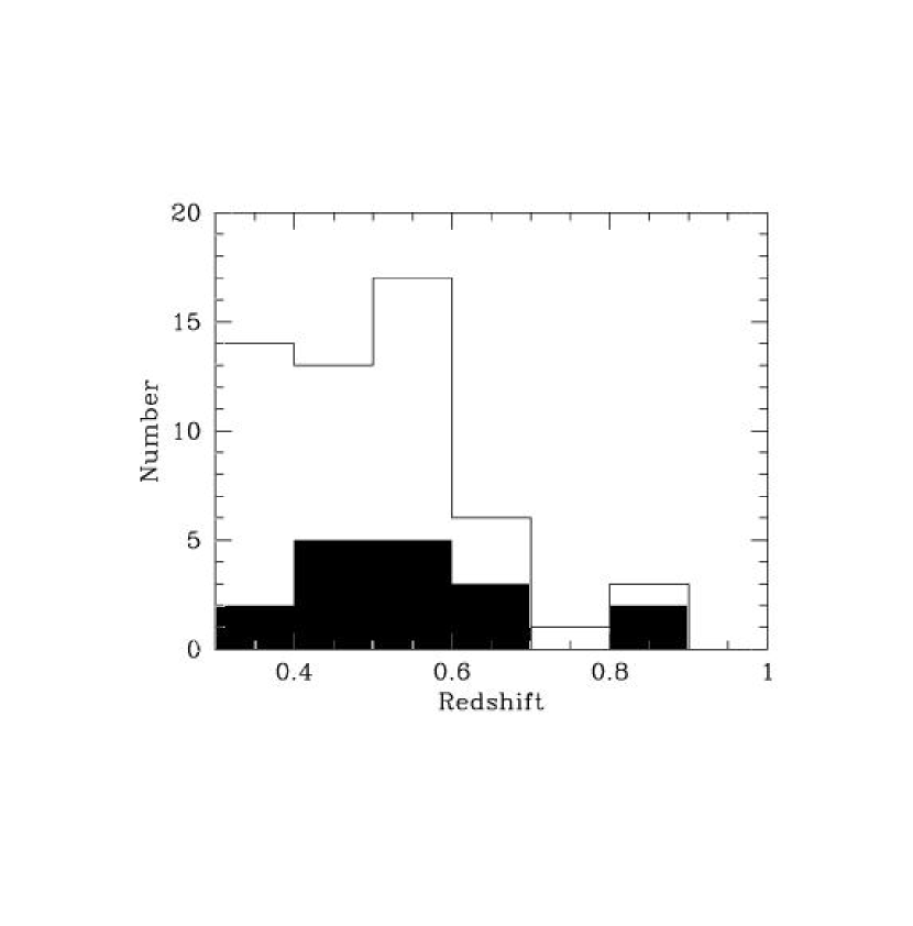
Figure 1.— The redshift distribution of our sample of BCGs with spectroscopic redshifts (filled histogram) and the full sample (open histogram).

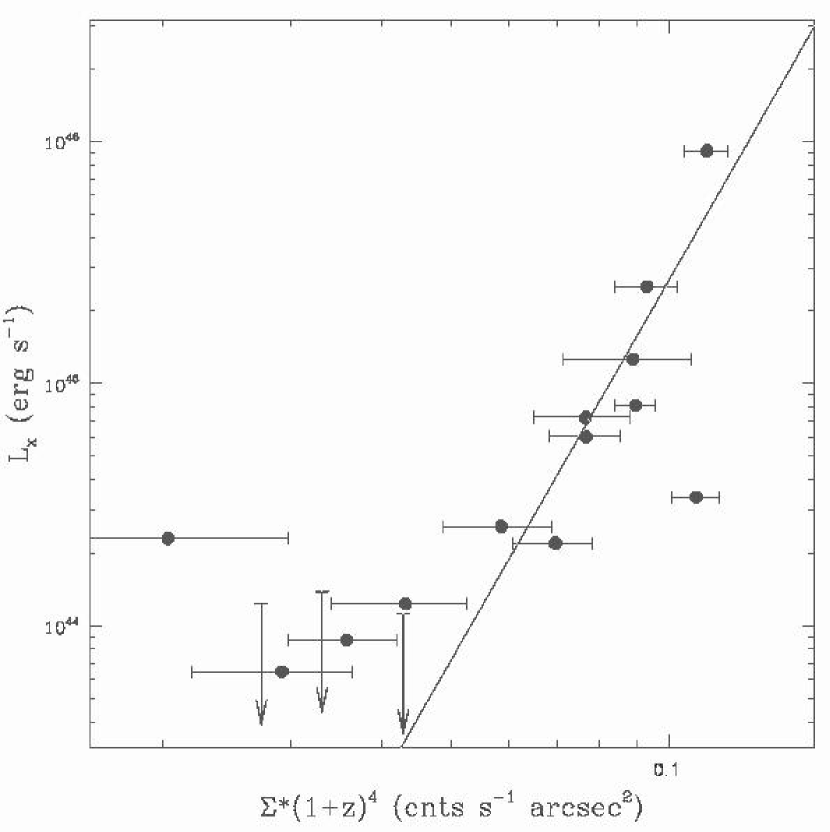
Figure 2.— Comparison of L_x with $\Sigma(1+z)^{5}$ for 17 known x-ray clusters for which we have drift scan data. L_x is the cluster x-ray luminosity in the EMSS band (0.3-3.5 keV) and $\Sigma$ is the peak surface brightness of the detection fluctuation. The line is the least squares fit to the data.

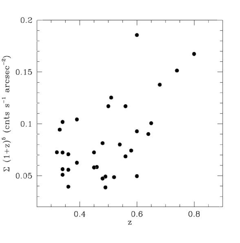
Figure 3.— Comparison of $\Sigma(1+z)^{5}$ with $z$ for clusters used in this work. Because $\Sigma(1+z)^{5}$ correlates with L_x, our sample is biased toward more massive systems at high redshift.

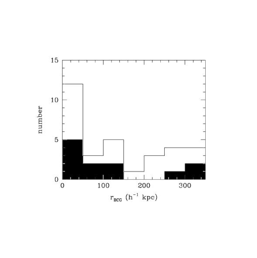
Figure 4.— The distribution of the radial separation of the BCG from the cluster center, $r_{BCG}$, for all color-selected BCGs (open histogram) and for those with $z_{spec}$ only (filled histogram).

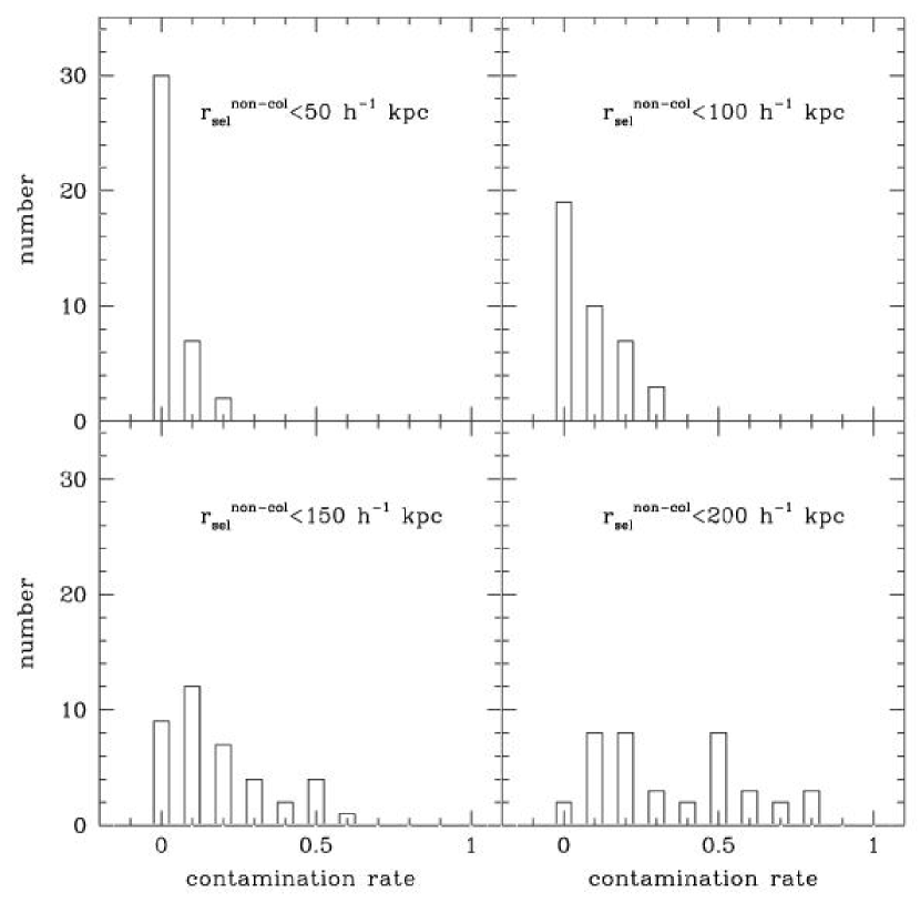
Figure 5.— The distribution of contamination rates for four searching radii: $r^{non-col}_{sel}=50h^{-1}$ kpc (upper left panel), $r^{non-col}_{sel}=100h^{-1}$ kpc (upper right panel), $r^{non-col}_{sel}=150h^{-1}$ kpc (lower left panel), and $r^{non-col}_{sel}=200h^{-1}$ kpc (lower right panel). The contamination rate is defined as the fraction of times that a galaxy within the search radius is brighter than the color-selected BCG (see text for details).

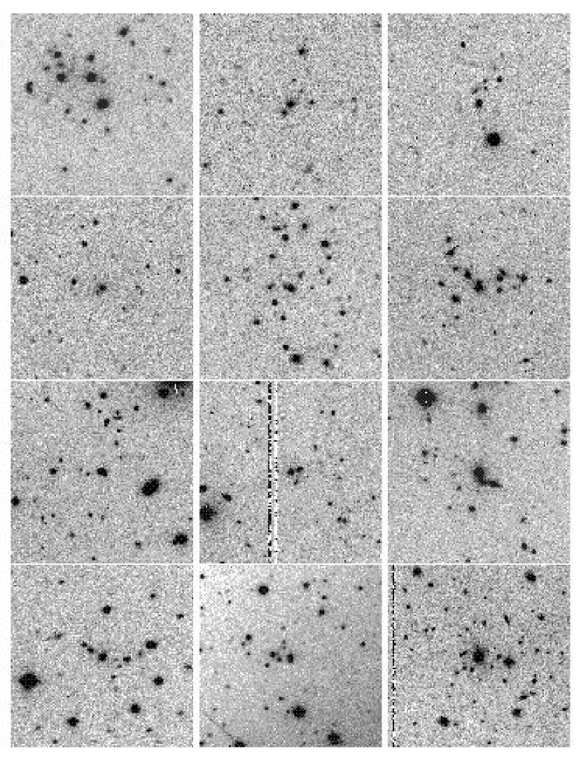
Figure 6.— Postage stamp images of the BCGs used in this work. All images are in the $I$-band except 1100+4620 which is imaged in $K^{\prime}$ . The orientation of the images is such that north points up and east to the right. The images are of (starting at the top, from left to right): 0915+4738, 0936+4620, 1002-1245, 1002-1247, 1005-1209, 1007-1208, 1012-1243, 1012-1245, 1014-1143, 1015-1132, 1017-1128, 1018-1211. (Due to size restrictions the astro-ph version only shows one of the set of five panels. The others are available at ngala.as.arizona.edu:/dennis/clusters.html or the published version)

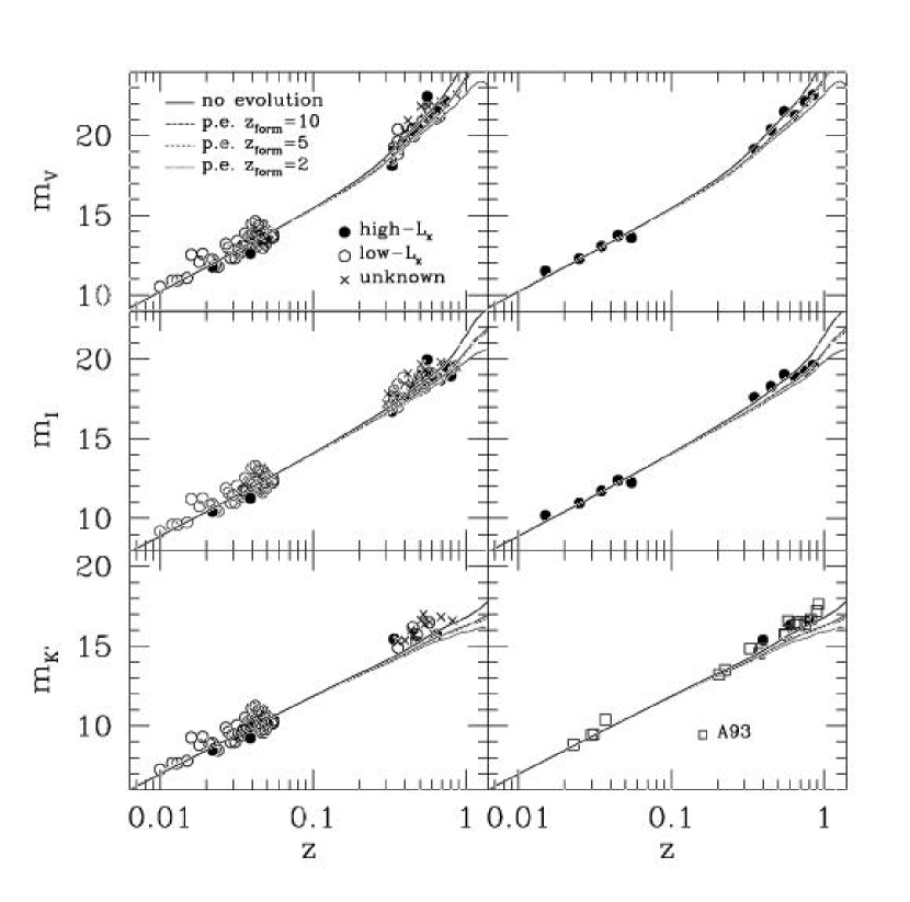
Figure 7.— The $V$-band (upper panels), $I$-band (center panels), and $K^{\prime}$-band (lower panels) Hubble diagrams for BCGs from high-L_x clusters (left panels, filled circles), low-L_x clusters (left panels, open circles), and clusters for which L_x cannot be estimated (left panels, crosses). The threshold between high-L_x and low-L_x is $2\times 10^{44}$ ergs s^-1. The errors in the photometry are negligible, but an error in $z_{phot}$ of 0.07 corresponds to $\Delta m_{I}\sim 0.3$ mag at $z\sim 0.6$. The BCG luminosities are compared to the spectral synthesis model predictions of Bruzual & Charlot (1993) for an elliptical galaxy experiencing passive evolution and no-evolution. The low redshift points are BCGs from PL95 for which the host cluster has x-ray data and are used to normalize the models. In the right panels, our data are binned in $\Delta z=$0.1 for the $V$- and $I$-bands (while $\Delta z=0.01$ for PL95). For the $K^{\prime}$ -band we bin the data in $\Delta z=0.2$ and compare to the $K$-band BCG sample of A93 (open squares), which is not binned. The error bars, which are $\sigma_{mean}$ of the binned data, are smaller than the points and are omitted.

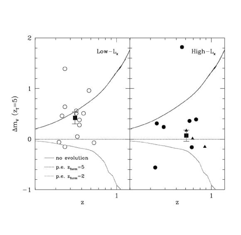
Figure 8.— BCG $V$ magnitude residuals for low-L_x clusters (left panel) and high-L_x clusters (right panel). Because we detect only very massive clusters at high redshift, clusters without measured values of $\Sigma$ at $z\geq 0.6$ are included in the high-L_x sample (filled triangles). Residuals are defined as $\Delta m=m_{BCG}-m_{model}$, for a passive evolution model with $z_{form}=5$. The filled boxes are the mean magnitude residuals and have error bars that are $\sigma_{mean}$. The lines are the same as those in Figure 7.

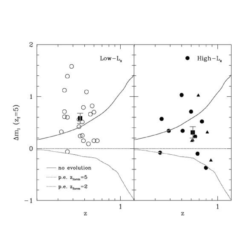
Figure 9.— Same as for Figure 8 but in the $I$-band

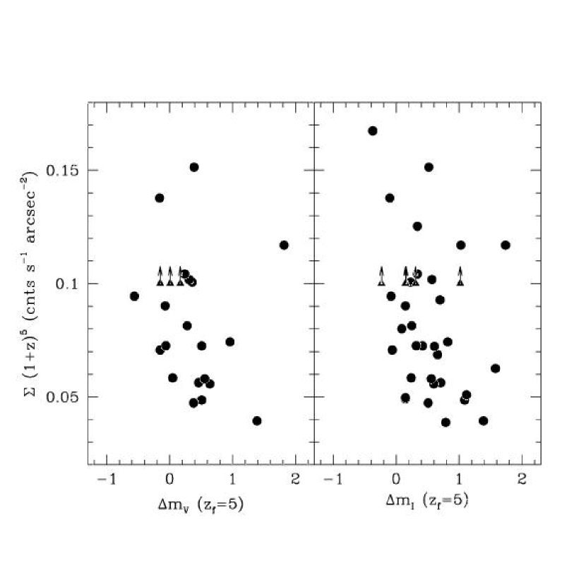
Figure 10.— Comparison of BCG magnitude residuals, $\Delta m=m_{BCG}-m_{model}$, in $V$ (left panel) and $I$ (right panel) with $\Sigma(1+z)^{5}$ for passive evolution with $z_{form}=5$. Filled triangles are BCGs at $z\geq 0.6$ without measured values of $\Sigma$. Because we are only sensitive to massive clusters at high redshift, we assign these BCGs lower limiting values of $\Sigma(1+z)^{5}=0.100$.

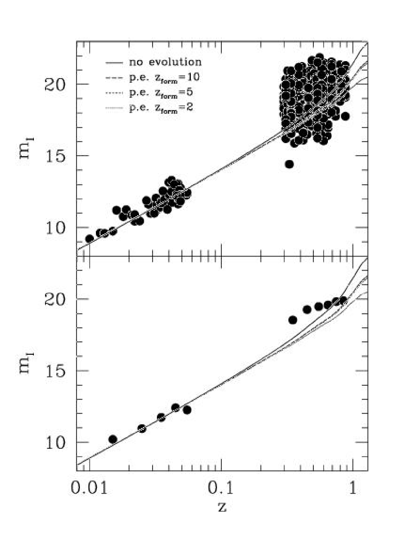
Figure 11.— $I$ Hubble diagram for the brightest field galaxies selected in random areas comparable to that of our clusters (upper panel). In the lower panel, the data are binned in $\Delta z=0.1$. The error bars, which are $\sigma_{mean}$ of the binned data, are smaller than the points and are omitted.

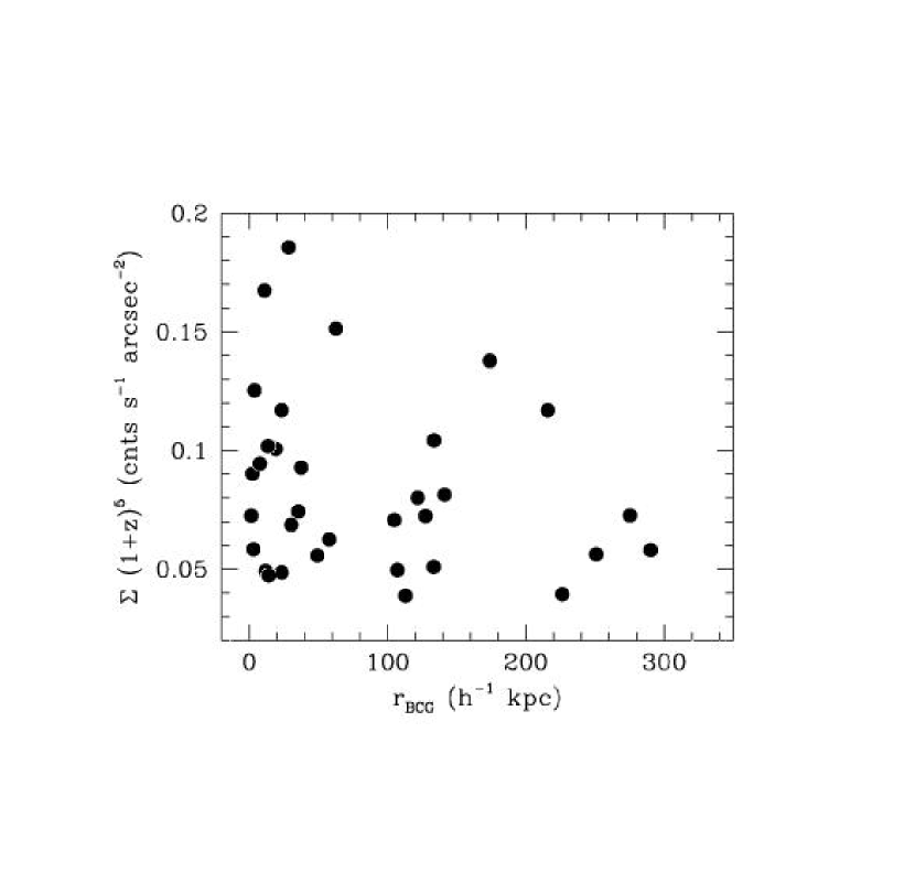
Figure 12.— Comparison of $\Sigma(1+z)^{5}$ with $r_{BCG}$. The lack of a statistically significant correlation between $\Sigma(1+z)^{5}$ and $r_{BCG}$ suggests that the measurements of $\Sigma$ are not biased by contamination from the BCG halo.

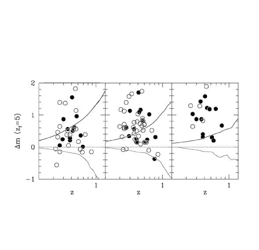
Figure 13.— BCG magnitude residuals in $V$ (left panel), $I$ (center panel), and $K^{\prime}$ (right panel) for clusters with $z_{spec}$ (filled circles) and $z_{phot}$ (open circles). Residuals are defined as $\Delta m=m_{BCG}-m_{model}$, for a passive evolution model with $z_{form}=5$. The lines are the same as those in Figure 7.

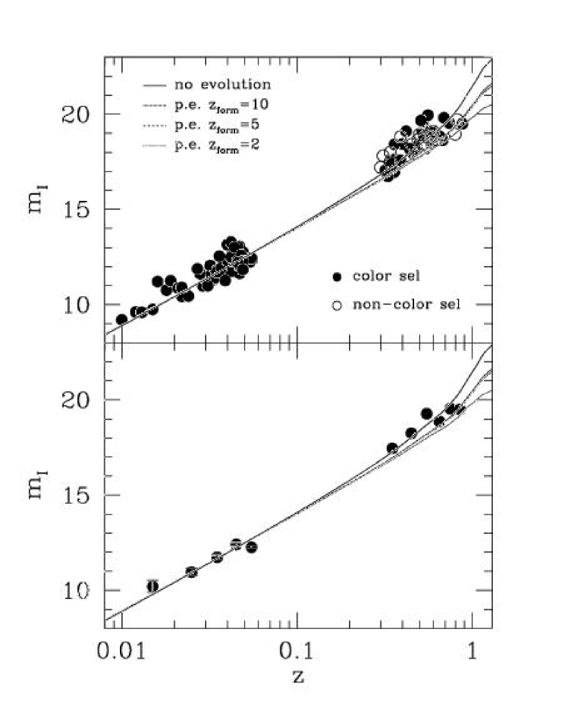
Figure 14.— The $I$-band Hubble diagram from Figure 7, differentiating between color-selected and non-color-selected BCGs. Symbols are the same as for Figure 7.

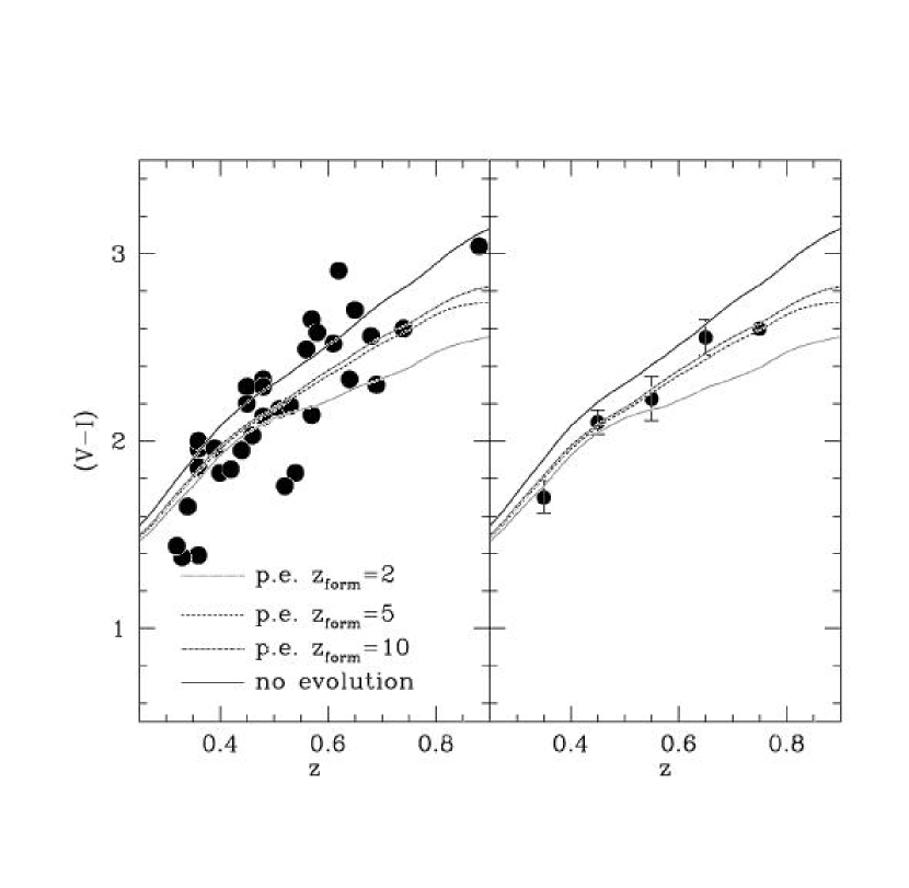
Figure 15.— BCG colors in $V-I$ compared to the spectral synthesis model predictions of Bruzual & Charlot (1993) for an elliptical galaxy experiencing passive evolution and no-evolution (left panel). In the right panel, the data are binned in $\Delta z=0.1$ and have error bars which are $\sigma_{mean}$ of the binned data.

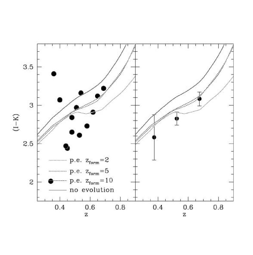
Figure 16.— BCG colors in $I-$$K^{\prime}$ compared to the spectral synthesis model predictions of Bruzual & Charlot (1993) for an elliptical galaxy experiencing passive evolution and no-evolution (left panel). In the right panel, the data are binned in $\Delta z=0.15$ and have error bars which are $\sigma_{mean}$ of the binned data.

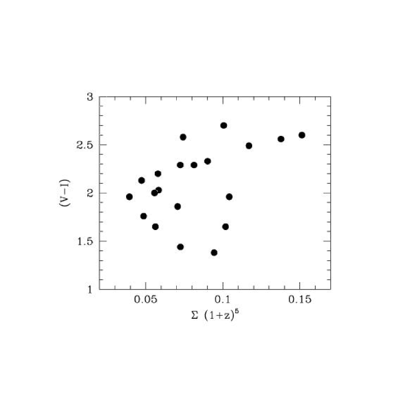
Figure 17.— Comparison of the colors of BCGs in $V-I$ with $\Sigma(1+z)^{5}$. There is no statistically significant correlation between the BCG colors and $\Sigma(1+z)^{5}$.

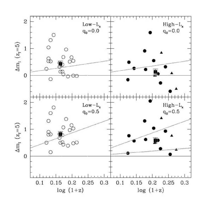
Figure 18.— BCG $I$ magnitude residuals for low-L_x clusters (left panels) and high-L_x clusters (right panels). Residuals are defined as $\Delta m=m_{BCG}-m_{model}$, for a passive evolution model with $z_{form}=5$ (solid line) assuming $\Omega_{m}=0.0,\Omega_{\Lambda}=0.0$ (upper panels) and $\Omega_{m}=1,\Omega_{\Lambda}=0$ (lower panels) and H${}_{0}=$50 km s^-1 Mpc^-1. Symbols are the same as for Figure 8. The filled boxes denote the mean magnitude residuals and have errorbars which are $\sigma_{mean}$ of the data. The dotted lines are the mass accretion rates predicted by ABK for low-L_x BCGs, while the dashed line is the mass accretion rate from BCM for high-L_x BCGs.

Table 1Observations

	RA	DEC	V	Seeing	I	Seeing	K	Seeing
Cluster	(JD2000)	(JD2000)	(min)	(′′)	(min)	(′′)	(min)	(′′)
0915+4738	09:15:51.94	+47:38:19.9	50	1.8	33	1.9	56	2.0
0936+4620	09:36:06.28	+46:20:43.2	80	2.5	80	1.9	64	2.0
0944+4732	09:44:21.83	+47:32:42.6	…	…	…	…	40	2.0
1002$-$1245	10:02:01.47	$-$12:45:35.1	120	1.4	60	1.4	…	…
1002$-$1247	10:02:27.14	$-$12:47:13.1	120	1.4	60	1.4	…	…
1005$-$1147	10:05:43.60	$-$11:47:43.1	…	…	60	1.2	…	…
1005$-$1209	10:05:49.72	$-$12:09:36.5	…	…	45	1.4	…	…
1006$-$1222	10:06:29.25	$-$12:22:13.7	…	…	45	1.4	…	…
1006$-$1258	10:06:18.79	$-$12:58:12.5	…	…	68	1.1	…	…
1007$-$1208	10:07:42.60	$-$12:08:36.0	…	…	40	1.3	…	…
1012$-$1243	10:12:14.58	$-$12:43:10.9	…	…	45	0.8	32	0.8
1012$-$1245	10:12:44.35	$-$12:45:37.9	30	0.9	30	0.7	…	…
1014$-$1143	10:14:56.31	$-$11:43:08.1	…	…	45	1.2	…	…
1015$-$1132	10:15:19.47	$-$11:32:55.5	…	…	60	1.3	…	…
1017$-$1128	10:17:45.31	$-$11:28:07.8	…	…	60	1.1	…	…
1018$-$1211	10:18:46.45	$-$12:11:52.8	40	1.2	40	0.6	…	…
1023$-$1303	10:23:10.11	$-$13:03:52.0	…	…	30	0.6	…	…
1024$-$1239	10:24:44.94	$-$12:39:55.6	40	1.1	40	0.9	…	…
1025$-$1236	10:25:08.83	$-$12:36:20.0	90	1.5	115	2.7	…	…
1027$-$1159	10:27:26.31	$-$11:59:33.6	90	1.5	105	1.8	…	…
1031$-$1244	10:31:50.26	$-$12:44:27.2	40	1.0	60	0.8	…	…
1032$-$1229	10:32:04.91	$-$12:29:43.8	120	1.8	115	1.8	…	…
…	…	…	…	…	15	1.0	…	…
1041+4626	10:41:03.79	+46:26:36.3	40	2.5	60	2.2	118	2.0
1059+4737	10:59:38.03	+47:37:38.6	50	3.3	50	2.0	55	2.0
1100+4620	11:00:57.36	+46:20:38.3	…	…	…	…	88	2.0
1136$-$1136	11:36:31.95	$-$11:36:07.7	30	1.3	30	1.1	…	…
…	…	…	…	…	20	1.1	…	…
1136$-$1145	11:36:47.07	$-$11:45:33.3	13	1.1	20	0.9	44	0.8
…	…	…	40	1.0	40	0.8	…	…
1136$-$1252	11:36:33.54	$-$12:52:03.3	20	0.8	20	0.6	20	2.0
…	…	…	…	…	20	1.4	…	…
1138$-$1142	11:38:06.59	$-$11:42:10.3	20	1.1	30	0.7	32	0.8
…	…	…	60	1.3	60	1.2	…	…
1138$-$1225	11:38:14.24	$-$12:25:53.9	90	1.2	120	2.0	…	…
1138$-$1228	11:38:44.70	$-$12:28:25.4	30	0.7	20	0.8	…	…
1139$-$1154	11:39:30.47	$-$11:54:25.0	30	0.9	30	0.8	10	2.0
1139$-$1217	11:39:56.84	$-$12:17:19.8	20	0.7	20	0.8	32	0.8
1145$-$1155	11:45:22.36	$-$11:55:52.1	20	0.7	20	1.0	50	2.0
…	…	…	40	1.2	30	0.8	…	…
1147$-$1252	11:47:16.98	$-$12:52:04.7	20	1.0	20	0.9	32	0.8
…	…	…	40	1.2	30	0.7	…	…
1149$-$1159	11:49:22.14	$-$11:59:19.3	3	0.9	10	0.9	…	…
1149$-$1246	11:49:06.18	$-$12:46:06.3	20	0.9	20	0.8	32	0.8
…	…	…	40	1.0	40	0.7	…	…
1208$-$1151	12:08:26.67	$-$11:51:25.6	90	1.4	68	1.2	…	…
1210$-$1219	12:10:12.73	$-$12:19:06.9	60	1.4	60	1.4	…	…
1211$-$1220	12:11:04.16	$-$12:20:47.7	…	…	45	0.8	…	…
1215$-$1252	12:15:41.08	$-$12:52:59.7	…	…	68	1.1	…	…
1216$-$1201	12:16:45.10	$-$12:01:17.3	…	…	45	1.3	…	…

Table 1Observations

	RA	DEC	V	Seeing	I	Seeing	K	Seeing
Cluster	(JD2000)	(JD2000)	(min)	(′′)	(min)	(′′)	(min)	(′′)
1219$-$1154	12:19:34.88	$-$11:54:22.9	…	…	60	1.3	…	…
1219$-$1201	12:19:44.49	$-$12:01:35.5	…	…	60	1.3	…	…
1221$-$1206	12:21:46.20	$-$12:06:12.7	…	…	45	1.2	…	…
1230+4621	12:30:16.26	+46:21:17.1	67	3.8	33	2.2	72	2.0
1326$-$1218	13:26:12.66	$-$12:18:22.5	40	0.9	50	0.9	36	0.8
1327$-$1217	13:27:57.33	$-$12:17:16.7	20	1.1	20	1.0	42	0.8
…	…	…	40	1.3	50	0.8	…	…
1329$-$1256	13:29:11.37	$-$12:56:22.0	90	1.6	95	1.4	20	2.0
…	…	…	45	1.1	30	1.0	…	…
1333$-$1237	13:33:01.92	$-$12:37:17.0	20	0.9	30	1.2	…	…
1404$-$1216	14:04:47.20	$-$12:16:21.4	90	1.5	60	1.3	…	…
1405$-$1147	14:05:11.38	$-$11:47:08.6	…	…	60	1.4	…	…
1406$-$1232	14:06:36.54	$-$12:32:39.7	…	…	45	1.4	…	…
1408$-$1209	14:08:17.86	$-$12:09:27.0	…	…	68	1.0	…	…
1408$-$1216	14:08:45.95	$-$12:16:08.8	…	…	68	1.0	…	…
1408$-$1218	14:08:50.62	$-$12:18:14.8	…	…	68	1.0	…	…
1412$-$1150	14:12:32.56	$-$11:50:16.2	…	…	8	1.2	…	…
…	…	…	…	…	30	0.8	…	…
1412$-$1222	14:12:25.92	$-$12:22:53.3	…	…	8	1.3	…	…
…	…	…	…	…	45	0.8	…	…
1412$-$1222.1	14:12:31.26	$-$12:22:15.8	…	…	45	0.8	…	…
1413$-$1244	14:13:08.59	$-$12:44:11.6	…	…	40	1.2	…	…
1416$-$1143	14:16:45.13	$-$11:43:40.0	…	…	40	1.3	…	…
1422+4622	14:22:24.18	+46:22:39.7	80	1.7	83	2.4	35	2.0
1519+4622	15:19:54.27	+46:22:20.4	…	…	15	2.3	45	2.0

Table 2BCG Data

Cluster	$z$	$\Sigma(1+z)^{5}$	mV	mI	m${}_{K^{\prime}}$	$V-I$	$I-$$K^{\prime}$
0915$+$4738	0.40	…	20.26	18.44	15.37	1.83	3.07
0936$+$4620	0.54	…	21.11	19.28	16.37	1.83	3.16
0944$+$4732	0.58	…	…	…	16.49	…	…
1002$-$1245	0.52	0.049	20.87	19.11	…	1.76	…
1002$-$1247	0.64	0.090	21.05	18.72	…	2.33	…
1005$-$1209	0.45	…	…	18.41	…	…	…
1007$-$1208	0.49	0.049	…	18.02	…	…	…
1012$-$1243	0.49	0.039	…	18.66	…	…	…
1012$-$1245	0.57	…	21.82	19.16	…	2.65	…
1014$-$1143	0.30	…	…	17.21	…	…	…
1015$-$1132	0.60	0.050	…	18.54	…	…	…
1017$-$1128	0.50	0.117	…	18.95	…	…	…
1018$-$1211	0.45	0.073	20.35	18.06	…	2.29	…
1023$-$1303	0.51	0.125	…	18.31	…	…	…
1024$-$1239	0.56	0.117	22.44	19.95	…	2.49	…
1025$-$1236	0.36	0.071	18.84	16.97	…	1.86	…
1027$-$1159	0.34	0.056	19.24	17.59	…	1.65	…
1031$-$1244	0.68	0.138	21.20	18.64	…	2.56	…
1032$-$1229	0.46	0.058	19.97	17.94	…	2.03	…
1041$+$4626	0.62	…	…	18.64	15.73	2.91	2.91
1059$+$4737	0.36	…	19.04	17.65	15.30	1.39	3.41
1100$+$4620	0.46	…	…	…	15.69	…	…
1136$-$1136	0.36	0.039	20.38	18.42	…	1.96	…
1136$-$1145	0.65	0.101	21.54	18.84	15.72	2.70	3.12
1136$-$1252	0.36	0.056	19.63	17.63	14.91	2.00	…
1138$-$1142	0.45	0.058	20.40	18.20	16.19	2.20	2.44
1138$-$1225	0.33	0.094	18.11	16.73	…	1.38	…
1138$-$1228	0.57	…	21.24	19.10	…	2.14	…
1139$-$1154	0.42	…	20.95	19.10	…	1.85	…
1139$-$1217	0.48	…	20.29	17.96	15.31	2.33	2.65
1145$-$1155	0.48	0.047	20.46	18.32	15.73	2.13	…
1147$-$1252	0.58	0.074	21.71	19.13	16.48	2.58	2.73
1149$-$1159	0.32	0.073	18.49	17.05	…	1.44	…
1149$-$1246	0.48	0.081	20.36	18.06	15.22	2.29	2.84
1208$-$1151	0.61	…	21.10	18.59	…	2.52	…
1210$-$1219	0.74	0.151	22.14	19.54	…	2.60	…
1215$-$1252	0.39	0.063	…	18.82	…	…	…
1216$-$1201	0.80	0.167	…	18.94	…	…	…
1219$-$1201	0.56	0.069	…	18.87	…	…	…
1221$-$1206	0.34	0.072	…	17.49	…	…	…
1230$+$4621	0.51	…	21.84	19.67	16.62	2.17	2.97
1326$-$1218	0.53	…	20.99	18.80	17.00	2.19	2.61
1327$-$1217	0.44	…	20.14	18.18	16.00	1.95	2.47
1329$-$1256	0.34	0.102	19.09	17.45	15.44	1.65	2.01
1333$-$1237	0.88	…	22.54	19.50	…	3.04	…
1404$-$1216	0.39	0.104	19.53	17.58	…	1.96	…
1408$-$1209	0.34	0.051	…	18.00	…	…	…
1408$-$1216	0.60	0.093	…	19.09	…	…	…
1408$-$1218	0.60	0.186	…	19.10	…	…	…
1412$-$1222	0.31	…	…	17.82	…	…	…
1412$-$1222.1	0.58	…	…	18.83	…	…	…
1416$-$1143	0.54	0.080	…	18.21	…	…	…
1422$+$4622	0.69	…	22.12	19.81	16.82	2.30	3.22
1519$+$4622	0.82	…	…	19.72	16.59	…	…

References

- a (93) Aragon-Salamanca, A., Ellis, R.S., Couch, W.J., & Carter, D. 1993, MNRAS, 262, 764, (A93)
- a (98) Aragon-Salamanca, A., Baugh, C.M., & Kauffmann, G. 1998, MNRAS, 297, 427 (ABK)
- b (96) Bertin, E, & Arnouts, S. 1996, A&AS, 117, 393
- b (92) Bower, R.G., Lucey, J.R., & Ellis, R.S. 1992, MNRAS, 254, 601
- b (00) Burke, D.J., Collins, C.A., & Mann, R.G. 2000, ApJ, 532L, 105 (BCM)
- b (93) Bruzual, G., & Charlot, S. 1993, ApJ, 405, 538
- c (98) Collins, C.A. & Mann, R.G. 1998, MNRAS, 297, 128 (CM)
- d (95) Dalcanton, J.J. 1995, Ph.D. Thesis, Princeton University
- d (97) Dalcanton, J.J., Spergel, D.N., Gunn, J.E., Schmidt, M., & Schneider, D.P. 1997, AJ, 114, 635
- d (96) van Dokkum, P.G. & Franx, M. 1996, MNRAS, 281, 985
- d (96) van Dokkum, P.G. & Franx, M. 2001, ApJ, 553, 90
- d (78) Dressler, A. 1978, ApJ, 223, 765
- g (00) Gonzalez, A., Zaritsky, D., Dalcanton, J., & Nelson, A. 2001a, in press
- g (00) Gonzalez, A., Zaritsky, D., Dalcanton, J., & Nelson, A. 2001b, submitted
- g (96) Graham, A., Lauer, T.R., Colless, M., & Postman, M. 1996 ApJ, 465, 534
- g (87) Gunn, J.E. et al. 1987, Opt.Eng., 26, 779
- h (80) Hoessel, J.G. 1980, ApJ, 241, 493
- h (80) Hoessel, J.G., Gunn, J.E., & Thuan, T.X. 1980, ApJ, 241, 486
- h (97) Hudson, M.J. & Ebeling, H. 1997, ApJ, 479, 621
- h (56) Humason, M.L., Mayall, N.U., & Sandage, A.R. 1956, AJ, 61, 97
- k (92) Kaastra, J.S., Asaoka, I., Koyama, K., & Yamauchi, S. 1992, å, 264, 654
- k (93) Kauffmann, G., White, S.D.M., & Guiderdoni 1993, MNRAS, 264, 201
- k (95) Kauffmann, G. 1995a, MNRAS, 274, 153
- k (95) Kauffmann, G. 1995b, MNRAS, 274, 161
- k (00) Kelson, D.D., Illingworth, G.D., van Dokkum, P.G., & Franx, M. 2000, ApJ, 531, 159
- k (01) Kelson, D.D., Illingworth, G.D., Franx, M., & van Dokkum, P.G., 2001, ApJ, 552, 17
- k (98) Kodama, T., Arimoto, N., Barger, A.J., & Aragon-Salamanca, A. 1998, A&A, 334, 99
- l (83) Landolt, A.U. 1983, AJ, 88, 439
- l (92) Landolt, A.U. 1992, AJ, 104, 340
- l (94) Lauer, T.R., & Postman, M. 1994, ApJ, 425, 418
- l (96) Lubin, L.M. 1996, AJ, 112, 23
- m (85) Mewe, R., Gronenschild, E.H.B.M., & van den Oord, G.H.J. 1985, A&AS, 62, 197
- m (85) Mewe, R., Lemen, J.R., & van den Oord, G.H.J. 1986, A&AS, 65, 511
- m (99) Mulchaey, J.S., & Zabludoff, A.I. 1999, ApJ, 514, 133
- n (00) Nelson, A.E., Gonzalez, A.H., Zaritsky, Z., & Dalcanton, J.J. 2001a, in press
- n (00) Nelson, A.E., Simard, L., Zaritsky, Z., Dalcanton, J.J., & Gonzalez, A.H. 2001b submitted
- o (76) Oemler, A. 1976, ApJ, 209, 693
- o (95) Oke, J., et al. 1995, Proc. SPIE, 2198, 178
- p (98) Persson, S.E., Murphy, D.C., Krzeminski, W., Roth, M., & Riecke, M.J. 1998, AJ, 116, 2475
- p (95) Postman, M, & Lauer, T.R. 1995, ApJ, 440, 28 (PL95)
- s (76) Sandage, A., Kristian, J., & Westphal, J.A. 1976, ApJ, 205, 688
- s (96) Schetman, S.A., Landy, S.D., Oemler, A., Tucker, D.L., Lin, H., Kirshner, R.P., & Schecter, P.L. 1996, ApJ, 470, 172
- s (98) Schlegel, D.L., Finkbeiner, D.P., & Davis, M. 1998, ApJ, 500, 525
- s (94) Schneider, D.P., Schmidt, M., & Gunn, J.E. 1994, AJ, 107, 124
- s (86) Schombert, J.M. 1986 ApJS, 60, 603
- s (97) Smail, I., Dressler, Al, Couch, W.J., Ellis, R.S., Oemler, A., Butcher, H., & Sharples, R.M. 1997, ApJS, 100, 213
- s (98) Standard, S.A., Eisenhardt, P.R., & Dickinson, M. 1998, ApJ, 492, 461
- s (95) Stanford, S.A., Eisenhardt, P.R. & Dickinson, M. 1995, ApJ, 450, 512
- t (77) Tremaine, S.D. & Richstone, D.O. 1977, ApJ, 212 311
- v (99) van Dokkum, P.G., Franx, M., Fabricant, D., Kelson, D.D., & Illingworth, G.D. 1999, ApJ, 520, L95
- z (98) Zabludoff, A.I. & Mulchaey, J.S. 1998, ApJ, 498L, 5
- z (97) Zaritsky, D., Nelson, A.E., Dalcanton, J.J., & Gonzalez, A.H. 1997, ApJ, 480, L91
- z (96) Zaritsky, D., Shectman, S.A., & Bredthauer, G. 1996, PASP, 108, 104