Radio–Optically Selected Clusters of Galaxies

In order to study the status and the possible evolution of clusters of galaxies at intermediate redshifts ($z\sim 0.1-0.3$), as well as their spatial correlation and relationship with the local environment, we built a sample of candidate groups and clusters of galaxies using radiogalaxies as tracers of dense environments. This technique – complementary to purely optical or X-ray cluster selection methods – represents an interesting tool for the selection of clusters in a wide range of richness, so to make it possible to study the global properties of groups and clusters of galaxies, such as their morphological content, dynamical status and number density, as well as the effect of the environment on the radio emission phenomena. In this paper we describe the compilation of a catalogue of $\sim 16\,000$ radio sources in the region of the South Galactic Pole extracted from the publicly available NRAO VLA Sky Survey maps, and the optical identification procedure with galaxies brighter than $b_{\mathrm{J}}=20.0$ in the EDSGC Catalogue. The radiogalaxy sample, valuable for the study of radio source populations down to low flux levels, consists of $1288$ identifications and has been used to detect candidate groups and clusters associated to NVSS radio sources. In a companion paper we will discuss the cluster detection method, the cluster sample as well as first spectroscopic results.

1 Introduction

One of the major topics in modern cosmology concerns the dynamical status and evolution of groups and clusters of galaxies, as well as their abundance and spatial distribution, their morphological content and interactions with the environment. Groups and clusters of galaxies are indeed the largest, gravitationally bound, observable structures, and by studying their properties and the processes underlying their formation much can be understood about the global cosmological properties of the universe.

In recent years, significant efforts have been made in searching for clusters at high redshifts; nevertheless the general properties and the physical processes at work in these large scale structures at moderate $z$ are still unclear. To this aim, it is of fundamental importance to gather cluster samples representative of different dynamical structures – from groups to rich clusters – in a wide range of redshift and covering large areas of the sky.

First attempts to build wide-area cluster samples, like the ACO/Abell catalogue (Abell et al. Abell (1989)), were based on visual inspection of optical plates and only recently the first catalogues obtained through objective algorithms appeared ( EDCC, Lumsden et al. Lumsden (1992); APM, Dalton et al. Dalton (1994)). The selection based on optical plates, however, limits the redshift range to about $z<0.2$ and suffers from misclassifications due to projections effects along the line of sight, resulting on one side in spurious cluster detection and, on the other side, in wrong estimates of the cluster richness, that can affect the reliability of the derived cosmological parameters (van Haarlem et al. van Haarlem (1997)). Alternatively, cluster samples at higher redshift have been built using a matched filter algorithm which makes use of both positional and deep multiband CCD photometric data over selected areas of few square degrees (Postman et al. Postman (1996); Scodeggio et al. Scodeggio (1999)).

Also, to find candidate clusters at intermediate redshift through color diagrams alone could bias the selection against clusters with a high fraction of blue galaxies, whose presence can be due to the occurrence of the Butcher–Oemler effect (Butcher & Oemler Butcher (1984)) or to the fact that the cluster itself can be in the process of formation.

The X-ray emission properties of the hot intracluster medium have been widely used to build distant cluster samples, but this technique suffers from the limited sensitivity of wide-area X-ray surveys and from the possibility of evolutionary effects (Gioia et al. Gioia (1990); Henry et al. Henry (1992); RDCS, Rosati et al. Rosati (1998)).

Even more critical is the selection of groups of galaxies: these structures – which represent a sort of “bridge” between rich clusters and the field – are of major interest for the understanding of galaxy interactions and evolutionary processes, but their detection is particularly difficult even at moderate redshifts due to their very low density contrast with respect to field galaxies distribution.

A different approach – complementary to purely optical or X-ray cluster selection methods – is the use of radiogalaxies as suitable tracers of dense environments. In recent studies (Prestage & Peacock Prestage (1988); Hill & Lilly Hill (1991); Allington–Smith et al. Allington–Smith (1993); Zirbel Zirbel97 (1997); Miller et al. Miller (1999)) it has been shown that Faranoff–Riley I and II radio sources are found in different environments, and differ in the optical properties of their host galaxies as well. FRI sources are found on average in rich groups or clusters at any redshift, and are associated with elliptical galaxies, with the most powerful FRIs often hosted by a cD or double nucleus galaxy (Zirbel Zirbel96 (1996)). FRII radio sources are typically associated with disturbed ellipticals and avoid cD galaxies, and at $z\sim 0.5$ FRIIs are found in a wide range of environments, including many rich clusters which rarely, if ever, host a FRII radio source at low redshift (Zirbel Zirbel96 (1996); Hill & Lilly Hill (1991)).

Radio selection should not impact on the X-ray or optical properties of the cluster found in this way, since there is no significant correlation between the radio properties of galaxies within a cluster with its $L_{\mathrm{X}}$ (Feigelson et al. Feigelson (1982); Burns et al. Burns (1994)), or with richness of the cluster (Zhao et al. Zhao (1989); Ledlow & Owen Ledlow (1996)). Moreover, since no correlation exists between the properties of group members and the radio characteristics of the radiogalaxies, radio-selected groups can be used to study the general evolution of galaxies in groups (Zirbel Zirbel97 (1997)).

Radiogalaxies can thus be used as tracers of dense environments at any epoch, and the evolution of galaxy groups and clusters can be studied lessening those biases that are the main drawbacks of pure optical or X-ray selected cluster samples.

A further point that makes this selection technique interesting is the possibility to investigate the effects of the environment on the radio-emission phenomena. Zirbel (Zirbel97 (1997)) speculates the possibility of two distinct scenarios for the fueling of radio emission in FRI and FRII sources. The difference in the environments of FRII radio sources at low and high redshift suggests that the conditions to form such sources have changed with epoch, and the characteristics of their optical counterparts are consistent with the hypothesis of FRII radio emission being fueled by galaxy encounters. For FRI radio sources, it is suggested the possibility of them being drawn from different galaxy types, and being triggered by different mechanisms, depending on their power. The most powerful FRI sources are typically dominant galaxies and their environments seem to be consistent with the possibility of them being cooling flow galaxies: in this scenario, the cooling flow itself can provide the fuel for the radio source. The less powerful FRI sources do not always correspond to the first ranked galaxy, are not always found in the centre of the potential well, and some reveal signs of galaxy interactions (see e.g. Baum et al. Baum (1988)). It seems thus unlikely that the less powerful FRIs can be cooling flow galaxies, and the radio emission could be triggered by a different mechanism with respect to more powerful FRIs.

This scenario suggests that the radio source morphology is not only a function of the radio power, as suggested by theoretical models (Bridle & Perley Bridle (1984); Bicknell Bicknell84 (1984), Bicknell86 (1986)), but depends also on the epoch of observation, that is the density and evolution of the intracluster medium. In this sense, the study of radio-selected groups and clusters over a wide range in radio power may help in understanding the physics of radio emission and the relationships between different classes of AGN.

To build such a sample of radio-traced clusters, the new radio surveys NRAO VLA Sky Survey (NVSS, Condon et al. Condon (1998)) and Faint Images of the Radio Sky at Twenty–centimeters (FIRST, Becker et al. Becker (1995)) offer an unprecedented possibility to study a wide-area, homogeneous sample of radio sources down to very low flux levels, together with a positional accuracy suitable for optical identifications.

Recently, Blanton et al. (Blanton (2000)) looked for moderate to high redshift clusters associated with a sample of radio sources from the FIRST survey, having a bent-double radio morphology. The presence of a distorted radio structure may be the consequence of the relative motion of the host galaxy in the intracluster medium, or of tidal interactions with other cluster galaxies, and thus can be used as an indicator of the presence of a cluster or group surrounding the radio source. From R-band imaging of the field surrounding bent-double radio sources, Blanton et al. (Blanton (2000)) selected ten candidates for multislit spectroscopy, and for eight of them they found evidence of a cluster associated to the radiogalaxy, with measured richnesses ranging from Abell class 0 to 2. As FRI sources more frequently show a distorted morphology, this sample contains mostly FRI radiogalaxies. Moreover, due to its high resolution, the FIRST survey may resolve out extended sources, making the FRI/FRII classification difficult.

The lower angular resolution of the NVSS survey makes this survey more suitable than the FIRST for the detection of extended regions of low surface brightness. We used the publicly available radio maps in the NVSS to build a sample of radio-optically selected clusters associated to FRI and FRII radio sources over a wide area in the sky. In this paper we describe the compilation of a radio source catalogue and the optical identification procedure with galaxies in the EDSGC Catalogue (Nichol et al. Nichol (2000)) that led to the compilation of the radiogalaxy sample. In a companion paper (Zanichelli et al. Zanichelli (2001), Paper II) we will present the cluster selection method and the sample of candidate clusters we have obtained, as well as first spectroscopic results.

This paper is structured as follows: in Sect. 2 we give a description of the characteristics of NVSS radio data and discuss the need to compile a radio source catalogue in alternative to the NVSS publicly available one. The extraction of the radio source catalogue is presented in Sect. 3, together with a discussion on the classification of double radio sources. The radio source catalogue and its properties are discussed in Sects. 4 and  5. In Sect. 6 and following the optical identification procedure and the obtained radiogalaxy sample are described.

2 The radio data

In this work we make use of data from the NRAO VLA Sky Survey (Condon et al. Condon (1998)). The NVSS started in 1993 with the VLA in D and DnC configurations and has recently been completed. The NVSS covers the whole sky north of $\delta=-40\degr$ at the frequency $1.4$ GHz with resolution $45\arcsec$.

Data products consists of $2326$ $\approx 4\degr\times 4\degr$ maps in Stokes I, Q, and U with pixel size $15\arcsec$ and rms brightness fluctuations $0.45$ mJy beam^-1. The positional rms in Right Ascension and Declination varies from $<1\arcsec$ for relatively strong ($S>15$ mJy) point sources to $7\arcsec$ for the faintest ($S=2.3$ mJy) detectable sources.

The positional accuracy, together with the low flux limit and moderate resolution of the survey makes the NVSS particularly suitable for the detection of low-surface brightness extended structures and for the search of optical counterparts of radio sources.

A list of about $2\times 10^{6}$ discrete sources is available as well, and has been extracted from the survey images by fitting elliptical Gaussians to all significant peaks (Condon et al. Condon (1998)). In the compilation of this list, hereafter NVSS–NRAO catalogue, no attempt is made to classify sources according to their morphology (double or pointlike sources).

Nevertheless, when one wants to make optical identifications, a crucial point is the knowledge of the source structure. If a double source, for which we can expect to find the optical counterpart near the radio barycentre position, is erroneously treated as two single components, the identification procedure can lead to misleading results, thus seriously affecting the completeness and reliability of the identification program.

The blind use of a list of fitted components like the NVSS–NRAO catalogue is thus not optimal if one wants to get a radiogalaxy sample characterized by well defined statistical properties, suitable for further astrophysical applications. For this reason, we developed our own algorithm for the extraction of a radio source catalogue from the radio maps and for the morphological classification of the detected sources, as will be discussed in the next Sections.

3 The radio source extraction algorithm

The operations performed by the extraction algorithm are divided in five modules: the source detection, the 1-Gaussian fit module, the evaluation of fit reliability, the 2-Gaussian fit module and the classification of double sources. More details on the operations performed by the algorithm are given in Appendix A.

3.1 Source detection

The algorithm reads each NVSS FITS map, consisting in a $1024\times 1034$ pixel matrix ($1\mathrm{pixel}=15\arcsec$), and then looks for emission peaks: we adopted a threshold flux of $S_{\mathrm{P}}=2.5$ mJy beam^-1, corresponding to the $5\sigma$ level for the NVSS survey (rms noise on NVSS I images is $\approx 0.45$ mJy beam^-1, Condon et al. Condon (1998)). A different detection threshold has been applied to two sky regions where strong residual diffraction lobes due to the presence of a very bright ($\sim 2.5$ Jy) and extended source are found. To avoid detecting a large number of spurious sources, for these regions we evaluated the local noise and selected only those peaks with $S_{\mathrm{P}}\geq 5\sigma_{\mathrm{local}}$.

A submatrix of $15\times 15$ pixels ($\sim 3.8\arcmin\times 3.8\arcmin$) around each peak is built, defining the region over which the operations described in the next Sects. are executed.

3.2 Fit with one Gaussian component

A fit with a circular Gaussian function of fixed ${\rm FWHM}=45\arcsec$ is performed over each submatrix (see Appendix A); the FWHM of the fitting function has been chosen to reproduce the nominal beam of the NVSS.

The use of a fixed FWHM has the consequence that it is not possible to determine the angular dimension – and thus the integrated flux – of the radio sources. Nevertheless, some tests showed that the use of a Gaussian of variable size is not advantageous when fitting sources at low flux levels ($\mathrel{\hbox to0.0pt{\lower 3.0pt\hbox{$\sim$}\hss}\raise 2.0pt\hbox{$<$}}8\sigma$), whose resulting positions and fluxes were found to be inaccurate. We decided thus to fix the dimensions of the fit function and to perform a fit with two Gaussian components in those cases when the one-component fit was not satisfactory. In Sect. 3.3 the criteria for performing a 2-component fit are described.

Input parameters for the 1-component fit are $x$ and $y$ peak pixel coordinates of the submatrix central point, and the measured flux at that pixel. For each source, the algorithm computes the fit rms $\Sigma_{\mathrm{1fit}}$ (see Appendix A), which is used as a discriminant for the execution of the 2-Gaussians fit.

3.3 Fit reliability

Inspecting the results obtained from the 1-component fit for some test sources, we found that they are not satisfactory in terms of positional and photometric accuracy when the fit rms $\Sigma_{\mathrm{1fit}}>0.6$ mJy pixel^-1. The distribution of $\Sigma_{\mathrm{1fit}}$ values in different flux bins showed that the percentage of sources with $S_{\mathrm{P}}<5.0$ mJy beam^-1  for which $\Sigma_{\mathrm{1fit}}\geq 0.60$ mJy pixel^-1 is reasonably low, of the order of $10\%$. We thus decided to apply a 2-component fit only to those sources with both $\Sigma_{\mathrm{1fit}}>0.60\leavevmode\nobreak\ {\rm mJy\leavevmode\nobreak\ pixel^{-1}}$ and $S_{\mathrm{P}}\geq 5.0\leavevmode\nobreak\ {\rm mJy\leavevmode\nobreak\ beam^{-1}}$. If it happens that $\Sigma_{\mathrm{2fit}}>\Sigma_{\mathrm{1fit}}$ ($\approx 4\%$ of these sources), then the 1-component solution is restored.

There are however two categories of sources for which the above criterion did not guarantee good results with the 1-component fit, and required a different approach: these cases are what we called “extended” and “multiple” sources.

When in presence of “extended” sources, whose flux distribution presents a “plateau” instead of a well defined maximum, the algorithm can detect more than one emission peak, and attempts to perform as many fits: this happens to about the $6\%$ of the sources fitted with 1 Gaussian component, with no dependence on their flux. It has been possible to identify two different situations: if the distance between the fitted positions is less than $4\arcsec$ then is always $\Sigma_{\mathrm{1fit}}<0.60$ mJy pixel^-1. For distances between $4\arcsec$ and $45\arcsec$, on the contrary, at least one fit has $\Sigma_{\mathrm{1fit}}>0.60$ mJy pixel^-1. In the first case we verified that $1$ Gaussian with fixed FWHM reproduces the source correctly: the 1-component fit is considered valid, by assigning to the radio source the position of the barycentre of the multiple fits. In the second case, the effect of the source extension is not negligible and the highest values of $\Sigma_{\mathrm{1fit}}$ and $S_{\mathrm{P}}$ among those fitted are attributed to the source, which is thus forced to the 2-component fit.

A further class of sources, the “multiple” ones, has been identified during the implementation of the 2-component fit module: the dimension of the fit submatrix is such that the number of times it contains two sources is not negligible. We found that the presence of more than one source in the same fit submatrix seriously affects the minimization process and the accuracy of fitted parameters.

We took into consideration these situations by introducing the following criterion: all those sources having a neighbour inside $2.5\arcmin$, with at least one of them having $\Sigma_{\mathrm{1fit}}>0.6$ mJy pixel^-1, are considered “double”. In such a case, a new fit submatrix is defined around the central position between the two components and the source is forced to the 2-component fit. A distance of $2.5\arcmin$ guarantees that the structure of both components is well represented in the region defined by the fit submatrix.

To keep track of the different operations and adopted criteria, multiple and extended sources have been marked with control flags. A further analysis of the classification of double sources has been made as the final step in the construction of the radio source catalogue (see Sect. 3.5).

3.4 Fit with two Gaussian components

The 2-component fit models sources with two Gaussian functions, each having ${\rm FWHM}=45\arcsec$. Input parameters needed to describe the two functions are: $x$ and $y$ peak pixel coordinates of the submatrix central point, peak flux, distance in $x$ and $y$ between the two components (in pixels from the barycentre), logarithmic ratio of fluxes of the two components. Obviously, this amounts to assume that the brightness distribution of the source is modelled as the sum of two pointlike sources.

Even if for true double radio sources it is seldom found a flux ratio $S_{\mathrm{1}}/S_{\mathrm{2}}>4$, we allowed this parameter to be as high as $10$, with a lower limit for the flux of a single component $S_{\mathrm{P}}=1.5$ mJy beam^-1. This choice proved to be useful to correctly fit the flux of those “extended” sources discussed in Sect. 3.3. In fact, due to our choice of fixed–size Gaussian functions, when dealing with “extended” sources for which a second peak is not detected, the extraction algorithm may need a second component to correctly fit the source flux.

For each double source the algorithm evaluates total flux and barycentre position, as well as flux, coordinates and separation of the two components. The fit rms $\Sigma_{\mathrm{2fit}}$ is computed similarly to what is done for the 1-component fit; if $\Sigma_{\mathrm{2fit}}\geq\Sigma_{\mathrm{1fit}}$, and depending on the source control flags (if there are any), the 1-component fit may have been considered valid.

Figure 1: Distribution of the separation between components, $D$, for $660$ double catalogue radio sources (solid line) and $409$ random doubles (dashed line), belonging to the $6$ maps we examined (see text).

3.5 Classification of double radio sources

The distinction made by the algorithm between single or double sources is strongly influenced by the sky distribution of radio sources and by the characteristics of the fit procedure, so that a certain number of spurious associations classified as double on the basis of a positional coincidence of single, non interacting components is expected. A further step in the compilation of the radio source catalogue is thus the estimate of the fraction of double radio sources that could have been so classified on the basis of the chance coincidence of two unrelated sources.

Figure 2: Histogram of fluxes for pointlike (a) and double (b) radio sources in the catalogue. There are $4$ pointlike sources with $LogS_{\mathrm{P}}>3.0$ and $1$ double source with $LogS_{\mathrm{P}}>3.4$ not shown in these plots.

Given the observed surface density of NVSS radio sources, and under the hypothesis that all of them are single sources, we looked at the probability that a source has by chance a neighbour assuming a completely random sky distribution. We considered regions of $4\degr\times 4\degr$ belonging to $6$ NVSS maps we analyzed. For each region we generated $5$ random samples each containing as many positions as the detected NVSS sources (i.e. $1\times n_{\mathrm{single}}+2\times n_{\mathrm{doubles}}$), associating to them values of the flux randomly chosen among the measured ones. We then looked for pairs in the random samples, i.e. sources having a neighbour inside $2.5\arcmin$, that is the maximum distance we allowed for the classification of a double source.

We detected an average of $409$ spurious doubles over the $6$ maps we took into consideration for this analysis. Over the same sky region, there are $660$ double radio sources in the catalog. In Fig. 1 the distributions of the distance between components for catalogue double sources and random double sources are shown.

We distinguish three different contamination situations depending on the separation $D$ between the radio components. When $D\leq 50\arcsec$ the mean contamination is about $13\%$ and we decided to keep as valid the algorithm classification: hereafter we will call these “close” double radio sources. For separations larger than $100\arcsec$ the probability of chance coincidence is such that we can consider all of them as spurious doubles: the $709$ radio sources belonging to this interval have thus been included as two single components among the list of single sources. In the interval between $50\arcsec$ and $100\arcsec$ a decision can hardly be made: the contamination rate for these radio sources is high ($\sim 61\%$) but the number of expected true doubles is not negligible. In order not to miss the corresponding optical identifications, we kept these sources (hereafter “wide” doubles) among the double ones, but for this group we followed a more careful procedure during the search of optical counterparts (see Sect. 7).

Our estimate of the number of random doubles, derived under the assumption of a uniform sky distribution of radio sources, does not take into account any effect due to clustering properties of radio sources. However, there is indication that the clustering of radio sources on angular scales greater than the NVSS resolution is weak (Magliocchetti et al. Magliocchetti98 (1998)), and thus it should not significantly alter our results.

Due to our choice of a maximum separation between radio source components of $100\arcsec$, our catalogue of double radio sources does not include the class of “giant” doubles. For a reliable detection of such sources, additional radio data with a better angular resolution than that provided by the NVSS survey alone would be needed, to allow the determination of the morphological type and of the compact core component necessary for the identification of the optical counterpart. Samples of giant radio sources have been selected on the basis of many different criteria on their angular size, radio power and optical magnitude (see e.g. Cotter et al Cotter (1996); Machalski et al. Machalski (2001)) so that it is not straightforward to give an estimate of the expected number of missed giants in our catalogue.

4 The radio source catalogue

The extraction algorithm has been applied to $31$ NVSS maps in the region of the South Galactic Pole. The algorithm classified as double $3371$ radio sources: among these, $709$ have distance between components $\geq 100\arcsec$ and have been included in the list of pointlike radio sources.

The resultant catalogue consists of $13\,340$ single sources and $2662$ double radio sources over $\approx 550$ sq. degrees of sky. The distribution of peak fluxes is shown in Fig. 2. The flux do not include any correction for the “CLEAN bias” ($\approx-0.3$ mJy beam^-1  for the NVSS): this has been taken into account when comparing our catalogue with the list of NVSS source components distributed by the NRAO (see Sect. 5).

The catalogue is complete down to the NVSS flux limit $2.5$ mJy beam^-1  and, as can be seen in Fig. 3, positional uncertainties estimated by the algorithm are in good agreement with those expected for NVSS sources (Condon et al. Condon (1998)).

The electronic version of the radio source catalogue is available at the Centre de Donnees de Strasbourg (CDS).

5 Tests on the catalogue

As the accuracy in positions and fluxes can influence the photometric completeness of the radio source catalogue as well as reliability and completeness of the optical identifications, before looking for radio source counterparts some tests to verify the algorithm stability and reliability in computing positions and fluxes have been performed on the catalogue.

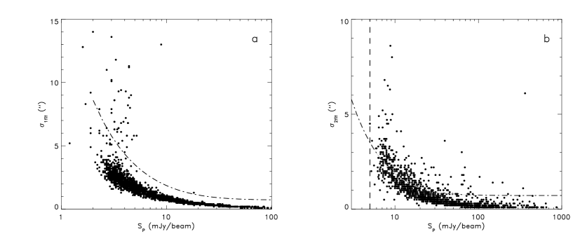
Figure 3: Positional uncertainties estimated by the radio source extraction algorithm for single (a) and double (b) radio sources as a function of peak flux. The dot-dashed line represent the errors derived from the formulae in Condon et al. Condon (1998). In (b) the dashed vertical line represents the flux limit for the $2$ components fit (see Sect. 3.4).

Figure 4: a Distribution of differences in Right Ascension for $323$ pointlike radio sources in our catalogue with respect to NVSS–NRAO catalogue positions. b NVSS–NRAO fluxes vs. radio source catalogue ones for the same set of sources. There are $4$ off-plot sources brighter than $160$ mJy beam^-1.

5.1 Comparison with the NVSS–NRAO catalogue

A first test to asses the accuracy of fluxes and positions computed by the radio source extraction algorithm described in the previous Sects. has been made with comparison to the NVSS–NRAO catalogue (Condon et al. Condon (1998)). The NVSS–NRAO catalogue does not provide any classification in single or double radio sources, and simply gives a list of components fitted with an elliptical Gaussian of variable size: for this reason, we restricted this quantitative analysis only to the single radio sources in our catalogue. A qualitative analysis of double radio sources has been made by visual inspection and described below.

We extracted from our catalogue a set of $323$ pointlike radio sources belonging to the central $3\times 3$ square degrees of the NVSS map I0016M24, and compared their positions and fluxes with those found in the NVSS–NRAO catalogue. To take into account the dependence of positional accuracy on the source flux, this analysis has been made in the three flux intervals $S_{\mathrm{P}}\leq 4$ mJy beam^-1, $4<S_{\mathrm{P}}\leq 8$ mJy beam^-1  and $S_{\mathrm{P}}>8$ mJy beam^-1. The modules of the mean differences in Right Ascension and Declination were found to vary from $\approx 0.5$ to $\approx 0.02\arcsec$ with a dependence on flux, with rms varying from $\sim 2\arcsec$ for the lowest fluxes to $\sim 0.3\arcsec$ for sources brighter than $8$ mJy beam^-1.

Photometric accuracy has been tested by comparing peak fluxes in the NVSS–NRAO catalogue with those determined by our extraction algorithm: these last result to be on average slightly underestimated, the median of the differences being $\Delta S_{\mathrm{P}}=-0.3$ mJy beam^-1, of the order of the “CLEAN bias” term for which the published NVSS–NRAO flux values have been corrected.

In Fig. 4 the offset distribution in Right Ascension, similar to the one in Declination, and the difference in fluxes between our catalogue and the NVSS–NRAO one are shown for the $323$ considered sources.

During this analysis we found that in some cases a bright pointlike radio source is split in more than one component by the NVSS–NRAO extraction algorithm. This fact can be ascribed to the use of a totally automatic extraction procedure, needed when managing such a huge amount of data. Nevertheless, it points out that the “blind” use of a component catalogue like the NVSS–NRAO one for optical identifications of radio sources can introduce contamination and incompleteness effects in the sample of of optical counterparts.

As the NVSS–NRAO catalogue does not make any attempt in classifying double radio sources, a similar quantitative comparison has not been possible for double systems and we limited our analysis to the visual inspection of $68$ cases of “close” and “wide” doubles in the catalogue. “Close” pairs are generally fitted with $1$ component in the NVSS–NRAO catalogue and we found a good agreement between the NVSS–NRAO component position and the barycentre in the radio source catalogue. A different situation exists for “wide” pairs in the radio source catalogue: their radio structure, as seen on the radio maps, is typical of classical double radio sources. In such cases, for which the NVSS–NRAO catalogue lists only the positions of the two components, the optical counterpart is clearly to be searched near the radio barycentre position and thus would be missed if one makes a blind use of the NVSS–NRAO catalogue.

5.2 Stability and reliability of the algorithm

A further test has been made on the radio source catalogue by using sources in the overlapping regions between adjacent maps to check the stability of the extraction algorithm in reproducing fluxes and positions.

We compared catalogue data relative to $120$ single sources (half of them with fluxes larger than $10$ mJy beam^-1) and $53$ double sources with those obtained by fitting the same sources with the AIPS task JMFIT. We again found consistency with what predicted for NVSS sources: errors on the positions of single sources vary from $\approx 3\arcsec$ at fluxes lower than $5$ mJy beam^-1, to $0.2\arcsec$ for $S_{\mathrm{P}}\geq 15$ mJy beam^-1. For the double sources we find slightly larger values, $\sim 2\arcsec$ for $S_{\mathrm{P}}\geq 15$ mJy beam^-1. We can conclude that both for pointlike and double radio sources in our catalogue, the positional accuracy is good enough to allow optical identifications with galaxies brighter than $b_{\mathrm{J}}=20.0$ down to the NVSS flux limit.

The variation of catalogue peak fluxes and peak fluxes obtained with JMFIT is $\mathrel{\hbox to0.0pt{\lower 3.0pt\hbox{$\sim$}\hss}\raise 2.0pt\hbox{$<$}}1\%$ for single sources, similar to the values found examining radio sources in the overlapping regions; for double sources the fractional variation reaches the $\mathrel{\hbox to0.0pt{\lower 3.0pt\hbox{$\sim$}\hss}\raise 2.0pt\hbox{$>$}}5\%$ for fluxes larger than $15$ mJy beam^-1. This higher value can be ascribed to a difficulty in representing the source with two Gaussians of fixed FWHM as the source flux increases. However, these results can be considered satisfactory as the uncertainties are not such to compromise the reliability of the optical identifications.

6 The optical identification procedure

The optical identification procedure has been applied separately to the three classes of NVSS radio sources in our catalogue: pointlike, “close” doubles and “wide” doubles. “Wide” doubles are in fact affected by a non-negligible probability of being erroneously classified as double systems by our extraction algorithm, that is, we do not know a priori when the optical counterpart is to be expected near the radio barycentre, which we assume as the most likely position if the classification is correct (Venturi et al. Venturi (1997); Prandoni et al. Prandoni (2001)) or near the components. We thus have followed a careful approach in the identification of these sources, as will be detailed in Sect. 7.

Figure 5: Radio-optical offsets in Right Ascension (a) and Declination (b) for $218$ barycentres of NVSS radio sources in the catalogue (empty areas) and $62$ contaminants from random samples (shaded regions), optically identified with galaxies inside a box of size $40\arcsec$.

“Close” doubles have a low probability of being spurious associations of single components, so that in principle they could be treated as the pointlike sources during the identification phase, by looking for counterparts near their barycentres. Nevertheless, pointlike and “close” doubles have been kept distinct in the identification phase, since we verified (see Sect. 6.2) that for “close” doubles it is not possible to fulfil the requirements of the Likelihood Ratio method (De Ruiter et al. DeRuiter (1977)). This method – to be applied in order to keep the contamination from radio-optical chance coincidence sufficiently low in the radiogalaxy sample – has been used only for the list of optical counterparts of pointlike radio sources.

In the next Subsections we discuss the properties of the optical data used for the compilation of the radiogalaxy sample and the determination of radio-optical positional uncertainties, necessary to define the optimal radius for the search of optical counterparts. More details on the Likelihood Ratio method and on results from simulated samples are given in Appendix B.

6.1 Optical data

Optical identifications of radio sources in the NVSS catalog have been made with galaxies in the Edinburgh–Durham Southern Galaxy Catalogue (EDSGC, Nichol et al. Nichol (2000)). The EDSGC lists photographic $b_{\mathrm{J}}$ magnitudes for $\approx 1.5\times 10^{6}$ galaxies over a contiguous area of $\sim 1200$ sq. degrees at the South Galactic Pole. For the construction of the catalogue glass copies of $60$ plates IIIa–J of the ESO/SERC Sky Survey at galactic latitude $|b_{\mathrm{II}}|\geq 20\degr$ have been digitalized with the microdensitometer COSMOS (MacGillivray & Stobie, MacGillivray (1984)). The automatic algorithm for star/galaxy classification implemented in COSMOS has been optimized so to achieve a completeness greater than $95\%$ and stellar contamination less than $12\%$ for magnitudes $b_{\mathrm{J}}\leq 20.0$. Magnitudes have been calibrated via CCD sequences, providing a plate-to-plate accuracy of $\Delta b_{\mathrm{J}}\simeq 0.1$ and an rms plate zero-point offset of $0.05$ magnitudes.

The EDSGC catalogue becomes rapidly incomplete above $b_{\mathrm{J}}\simeq 20.5$, thus we decided to consider only those galaxies with $b_{\mathrm{J}}\leq 20.0$. With this conservative choice, the properties of the final identification sample (in terms of optical completeness and contamination) are well consistent with the global ones of the EDSGC.

6.2 Positional uncertainties and search radius

The search radius for optical identifications must be carefully chosen as it affects the completeness and reliability of the obtained radiogalaxy sample (see Appendix B). The optimal search radius is usually chosen on the basis of the total positional uncertainties, i.e. the combination of the radio error (comprehensive of the uncertainty introduced by the fit) which depends on source flux, and the accuracy on optical positions.

To avoid any kind of assumption on this term, we empirically determined the radio-optical positional accuracies from the distribution of the measured radio-optical offsets. Given the uncertainty in the classification of “wide” double radio sources, we made this analysis only for pointlike and “close” double sources.

We have first identified the $13\,340$ pointlike radio sources in the catalogue with EDSGC galaxies brighter than magnitude $b_{\mathrm{J}}=20.0$, looking for the nearest object inside a large square region of size $40\arcsec$, centered on each radio position. The distributions of the observed radio-optical offsets in $\alpha$ and $\delta$ have been analyzed in different bins of radio flux, selected in order to contain approximately the same number of counterparts.

Table 1: Gaussian estimates of the total errors on coordinates, $\sigma_{\mathrm{\alpha}}$ and $\sigma_{\mathrm{\delta}}$, obtained from a fit on the $\Delta\alpha$ and $\Delta\delta$ distributions of optical identifications for catalogue pointlike radio sources. For each one of the $5$ considered flux intervals it is also given the mean number of contaminants per distance bin $C_{\mathrm{med}}/\mathrm{bin}$, estimated by means of the $4$ control samples, which represent the “pedestal function” over which the Gaussian distribution of the true identifications lies.

$S_{\mathrm{P}}$( mJy beam-1)		$C_{\mathrm{med}}/\mathrm{bin}$		$\sigma_{\mathrm{\alpha}}\leavevmode\nobreak\ {\rm(\arcsec)}$	$\sigma_{\mathrm{\delta}}\leavevmode\nobreak\ {\rm(\arcsec)}$
$S_{\mathrm{P}}\leq 3.5$		3		5.17	5.28
$3.5<S_{\mathrm{P}}\leq 4.6$		2		4.11	5.76
$4.6<S_{\mathrm{P}}\leq 7.5$		3		3.16	3.33
$7.5<S_{\mathrm{P}}\leq 15.0$		3		2.04	2.27
$S_{\mathrm{P}}>15.0$		3		2.21	1.88

Each offset distribution is the sum of two distinct distributions: a flat one due to the uniform distribution of spurious counterparts, plus a Gaussian one due to the true radio-optical associations. To estimate the rms of this Gaussian, which is the desired positional uncertainty, we first obtained an accurate measure of the mean level of contaminants by making optical identifications of randomly generated samples. We built $4$ control samples, each containing $13\,340$ random positions, and looked for spurious optical counterparts in the same way as for catalogue sources.

By fitting the offset distributions with a Gaussian function plus a constant pedestal, given by the the contamination level in that flux range obtained from the control samples, we evaluated the total positional uncertainties shown in Table 1.

Similar values have been obtained repeating this analysis for the $1530$ “close” double radio sources, i.e. looking for optical counterparts inside a box of size $40\arcsec$ centered on the radio barycentre, and using again random samples to evaluate the contamination level.

On the basis of the estimated positional uncertainties, for the optical identification procedure of NVSS radio sources we thus adopted a search radius of $15\arcsec$.

The Likelihood Ratio method has subsequently been applied to the list of counterparts of pointlike sources, to discard those cases that are statistically unlikely to be true radio-optical associations. The same method proved to be inapplicable to the counterparts of “close” doubles, as in this case the hypothesis of Gaussian-distributed positional uncertainty, required by the Likelihood Ratio method, is not satisfied. As can be seen from Fig. 5, in fact, an excess of true identifications is found in the “tails” of the offset distributions. These could correspond to identifications of distorted radio sources, like Head–Tails, whose morphology is not completely resolved at the low NVSS resolution.

7 The radiogalaxy sample

The list of NVSS pointlike radio sources identified with EDSGC galaxies brighter than $b_{\mathrm{J}}=20.0$ inside a circle of radius $15\arcsec$ consists of $1061$ candidate counterparts, with an average of $254$ contaminants from the control samples: the initial contamination is thus $24\%\pm 2\%$. To this list of optical counterparts and to the counterparts found in the control samples we applied the modified Likelihood Ratio method described in Appendix B, evaluating $LR$ for each source using the positional uncertainty relative to its flux (see Table 1).

The Likelihood Ratio cutoff value for rejecting a counterpart as unlikely to be true was found to be $LR=LR_{\ast}=1.9$. Out of the initial list of $1061$ candidates, the final sample of optical identifications of pointlike NVSS radio sources thus consists of $926$ counterparts satisfying the condition $LR_{\ast}\geq 1.9$, while the number of contaminants in this sample, given by the mean number of spurious identifications in the control samples which have $LR\geq 1.9$, is $C_{\mathrm{med}}(LR_{\ast}\geq 1.9)\approx 145$.

The contamination percentage in the final sample of $926$ optical counterparts of NVSS pointlike radio sources is thus $\sim 16\%\pm 1\%$, while due to the choice of the cutoff value for $LR$ we expect to lose $\sim 24$ true identifications. This corresponds to a completeness of $\simeq 97\pm 1\%$ and to a reliability of $\simeq 84\%\pm 1\%$: we conclude that, with respect to the initial list of $1061$ candidate counterparts, the use of the modified Likelihood Ratio has sensibly lowered the contamination level without discarding a large number of real radio-optical associations. The identification percentage, expressed as the ratio between the number of true identifications and the total number of sources for which we looked for an optical counterpart, is about $\theta_{\mathrm{pointlike}}=(926-145)/13340=6\%\pm 0.2\%$.

Figure 6: Optical identifications of double radio sources in the interval $50\arcsec<D<100\arcsec$: images are taken from the Digitized Sky Survey and contours represent radio emission in the NVSS. From left to right and from top to bottom: B00025, B01640, B01094, B02230, B02322, B02348, B00532, B00065, for which we identify the barycentre and one component with two different galaxies; B00258, B00698, B01631 for which we identify the barycentre and $1$ component with the same galaxy and the second component with a different galaxy, and finally B01471 for which the barycentre and the two components are identified with $3$ different galaxies (see text).

For the $1530$ “close” doubles we looked for an optical counterpart brighter than $b_{\mathrm{J}}=20.0$ at a distance $\leq 15\arcsec$ from the radio barycentre, finding $169$ identifications. The number of spurious identifications obtained from the control samples is $28\pm 5$: the contamination percentage in the sample of optically identified “close” double radio sources is then $16\%\pm 3\%$, while the identification percentage is $\theta_{\mathrm{bar}}=9\%\pm 1\%$, consistent at the $3\sigma$ level with the value found for pointlike sources.

The identification procedure of the $1132$ “wide” double radio sources has been made as follows: we first looked for an optical counterpart inside a radius of $15\arcsec$ both from the barycentre position and from the positions of the two components, and then inspected those cases where more than one identification is found for the same radio source.

We initially identified $232$ positions; in $156$ cases we identify either the barycentre or one (or both) the components: in such cases, we consider valid the identification even if this does not mean that we are keeping the true optical counterpart.

In the remaining cases, a puzzling situation emerges as we find a counterpart for both the barycentre and one component, or even for the barycentre and the two components, so that a decision on the most reliable identification is difficult to make. To discard or retain an identification, we decided to proceed as follows: when we identify the barycentre and $1$ component with the same galaxy ($25$ cases), we assume that this happens because in the extraction algorithm we allowed high flux ratios. In fact, when a common identification is found for the barycentre and for one of the components (normally the strongest) we consider valid the association with the barycentre, even if this is somewhat arbitrary. Large values of $S_{\mathrm{1}}/S_{\mathrm{2}}$, up to $10$, are a feature introduced by our extraction algorithm and are not representative of the true distribution of flux ratios for double radio sources (see discussion in Sect. 3.4). To perform an analysis of flux ratios and arm–length ratios, and to compare it with other samples, we would need radio maps with much better resolution.

In the $12$ cases when we identify the barycentre and one component with two different galaxies, or the barycentre and one component with the same galaxy but at the same time we find a different identification for the second component, or finally we identify separately both the barycentre and the two components, we decided which is the most likely identification by visually inspecting the field. These few cases are shown in Fig. 6.

When the radio source structure is similar to a “head–tail” morphology, we considered the counterpart associated to the component corresponding to the radio source “head”. In the presence of extended but symmetric radio morphologies we retain the identification in the barycentre. An example of spurious double can be represented by B1471 in Fig. 6, the only case where we identify at the same time the barycentre and the two components with different galaxies. In this case we considered valid the two counterparts associated to the components of the double source.

By applying these criteria, we obtained a list of $193$ optical counterparts of “wide” double radio sources. Because of the presence of an “intrinsic” radio contamination, and given the subjective method adopted in the selection of true counterparts, it is possible to give only a lower limit to the contamination present in this list of identifications. The number of spurious identifications is $A\times N\times\rho_{\mathrm{opt}}=\pi\times(15)^{2}\times(1132\times 3)\times 2.7\times 10^{-5}=65$, that is a contamination percentage of $\sim 28\%$.

A summary of the different contamination levels as well as the number of optical counterparts found for each radio morphology we are considering is given in Table 2.

The final radiogalaxy sample thus consists of $1288$ sources optically identified with galaxies brighter than $b_{\mathrm{J}}=20$ in the EDSGC: in Fig. 7 the magnitude and flux distributions for the radiogalaxy sample are shown. The overall contamination in the radiogalaxy sample is $\sim 18\%$. The identification percentage we find for NVSS sources is in agreement with what found by Magliocchetti & Maddox (Magliocchetti (2001)) for optical identifications of higher–resolution FIRST radio sources with APM galaxies in the equatorial region, once scaled to our radio flux and optical magnitude limits. In Paper II we will use a subset of our radiogalaxy sample, characterized by a higher reliability, to look for intermediate redshifts cluster candidates associated to NVSS radio sources.

8 Summary

Aim of this work is to build a sample of radio-optically selected clusters of galaxies at intermediate redshift in order to study the evolution and general properties of groups and clusters as well as the effect of the environment on the radio emission phenomenon. In this paper we have discussed the compilation of a radio source catalogue from $31$ NVSS radio maps covering the South Galactic Pole region, and the search of optical counterparts of these radio sources. The main reason to build a radio source catalogue alternative to the NVSS–NRAO publicly available one has been the need to classify radio sources according to their morphology – unresolved or double – so to properly search for their optical counterparts.

Our radio source catalogue has been built by detecting emission peaks above the detection threshold $S_{\mathrm{P}}\sim 2.5$ mJy beam^-1  and fitting Gaussian components with FWHM equal to the NVSS beam size to the selected peaks. The source detection algorithm first attempts a one-component fit to each peak and, depending on the root mean square of the fit and on the distance between two neighbour peaks, if necessary a two-components fit is performed.

Classification of double radio sources has been done by first allowing the separation between components to be as large as $2.5\arcmin$ and compiling a first list of “tentative” double sources. Then, given the NVSS low resolution, a detailed analysis to discriminate between pointlike and double sources has been done by studying the probability of classifying two single, non interacting components as a double system on the basis of their separation. From this analysis we found that the probability of two sources being a physically bound system is negligible when their distance is greater than $100\arcsec$. These doubles have been removed from the “tentative” list and included as single components among the unresolved sources while, on the opposite, the classification of double sources is correct for those systems having $D\leq 50\arcsec$ (“close” doubles). In the intermediate range $50\arcsec<D<100\arcsec$ the number of expected spurious and true double sources are equivalent. These cases (“wide” doubles) have been included among double sources but for them a more careful optical identification procedure has been performed.

Figure 7: Peak flux (a) and magnitude (b) distributions for the $1288$ NVSS radio sources optically identified with EDSGC galaxies. There are $67$ radiogalaxies brighter than $80$ mJy beam^-1  not shown in the flux histogram.

Table 2: The radiogalaxy sample: for each radio morphology class the number of optical identifications and the contamination level are shown. The last row gives these quantities for the whole sample.

Radio			N			Contamination
Morphology
Pointlike			926			16 $\pm$ 1$\%$
“Close” double			169			16% $\pm$ 3$\%$
“Wide” double			193			28$\%$
Total			1288			18 $\%$

The final radio source catalogue consists of $13\,340$ single and $2662$ double radio sources over $\approx 550$ sq. degrees of sky, and is complete down to $S_{\mathrm{P}}=2.5$ mJy beam^-1.

A quantitative test to assess the accuracy of the radio source extraction algorithm has been made comparing fluxes and positions of a set of radio sources in our catalogue with the correspondent values in the NVSS–NRAO catalogue. Since the NVSS–NRAO catalogue does not classify double radio sources this analysis has been possible for pointlike sources only. We found that our results are in agreement with the ones in the NVSS–NRAO catalogue, well inside the predicted errors for the NVSS (Condon et al. Condon (1998)). For what concerns double radio sources, we made a qualitative analysis by visually inspecting a set of “close” and “wide” doubles and looking at their characteristics in the NVSS–NRAO catalogue. We found a good agreement in flux and positions for “close” doubles, while in most cases “wide” ones clearly show a classical double radio morphology on the maps. In such cases, where the optical counterpart should be looked near the radio barycentre, the use of the NVSS–NRAO catalogue without a re-processing to detect double sources, would result in a loss of optical identifications and thus in a less complete radiogalaxy sample.

Optical identifications of radio sources in our catalogue have been made with EDSGC galaxies (Nichol et al. Nichol (2000)) down to a limiting magnitude of $b_{\mathrm{J}}=20.0$ and adopting a search radius of $15\arcsec$.

Different strategies have been applied for the search of optical counterparts of pointlike or double radio sources. For the latter, the probability of having classified as a double system two physically disjointed sources on the basis of their superposition in the sky is in fact dependent on the distance between the two components. The optical identification of the $13\,340$ pointlike radio sources led to a sample of $926$ radiogalaxies. The statistical completeness and reliability of this sample have been evaluated by means of the modified Likelihood Ratio method proposed by De Ruiter et al. (DeRuiter (1977)) (see Appendix B), to properly take into account the true optical surface distribution of galaxies in the sky. This sample is complete to $97\%\pm 1\%$ and reliable to $84\%\pm 1\%$, with an identification percentage of $6\%\pm 0.2\%$.

The optical identification of $1530$ “close” double radio sources (distance between components $D\leq 50\arcsec$) has been made looking for a counterpart near the barycentre position. For these sources, the probability of being a spurious double is low, $\mathrel{\hbox to0.0pt{\lower 3.0pt\hbox{$\sim$}\hss}\raise 2.0pt\hbox{$<$}}13\%$. We optically identified $169$ barycentres of “close” doubles; in this case it was not possible to apply the modified Likelihood Ratio method to evaluate the reliability and completeness of the sample. An estimate of the contamination level has been computed as the probability of chance radio-optical superposition on the basis of the average observed optical surface galaxy density. We found a contamination of $16\%\pm 3\%$ for optical identifications of “close” double radio sources.

Optical identifications of “wide” doubles (distance between components $50\arcsec<D<100\arcsec$) are made difficult by the high percentage of expected radio misclassification: the number of true radio associations is in fact comparable with the number of radio contaminants. We thus looked for optical counterparts both near the radio barycentre and near the radio components positions, visually inspecting those cases where more than one optical identification is found for the same radio source. We found a list of $193$ optical counterparts of “wide” double radio sources, with a contamination of the order of $\sim 28\%$: this contamination level must be seen as a lower limit, as it does not take into account the joint probability of having a optical spurious identification near the barycentre of a spurious double radio source.

The final sample thus lists $1288$ radiogalaxies and represents a valuable opportunity for the study of the multi-wavelength properties of the radiogalaxy populations down to a low flux level.

This sample has been used to look for galaxy clusters associated to NVSS radiogalaxies: in a following paper (Zanichelli et al. Zanichelli (2001)) we discuss the cluster selection strategy and the first observational results, that prove this technique to be a powerful tool for the selection of galaxy groups and clusters at intermediate redshift.

Appendix A the Gaussian Fitting Algorithm

To define flux and accurate positions of radio sources from NVSS maps, we developed a code which performs a Gaussian bidimensional fit by means of a minimization process. Starting from $M$ functions in $N$ variables, $f_{k}(x_{\mathrm{1}},x_{\mathrm{2}},...,x_{\mathrm{N}})$, the routine MINSQ (Pomentale, Pomentale (1968)) minimizes the sum:

$$\phi^{2}(x_{\mathrm{1}},x_{\mathrm{2}},...,x_{\mathrm{N}})=\sum_{k=1}^{M}\biggl{\{}f_{k}(x_{\mathrm{1}},x_{\mathrm{2}},...,x_{\mathrm{N}})\biggr{\}}^{2}$$ (1)

where $M\geq N\geq 2$. The minimization process is iterated until the difference between the function before and after the minimization is lower than a user-selected value (“stopping rule”), or until a pre-defined maximum number of iteration is reached. Each source to be fitted is represented with a circular Gaussian of ${\rm FWHM}=\sigma$ and peak amplitude $A$:

$$G(x,y)=A\leavevmode\nobreak\ e^{-{x^{2}+y^{2}\over 2\sigma^{2}}}$$ (2)

If the source image is composed of $M$ independent measures of the amplitude $a_{k}$, each one with a known associated error $\sigma$, the $f_{k}$ can be defined as:

$$f_{k}={[a_{k}-G(x_{k},y_{k})]^{2}\over\sigma^{2}}$$ (3)

Inserting this expression for the $f_{k}$ in the (1), the maximum-likelihood fit would be the one which minimizes the $\phi^{2}$. In our case, the errors on the individual measurements are not a priori known: as a first approximation we could assume that they are constant over the image and equal to the mean survey rms ($\approx 0.45$ mJy beam^-1), but this assumption fails in presence of bright sources. We thus expressed the $f_{k}$ functions simply as the unweighted quadratic differences between the data and the fit at each pixel:

$$\phi^{2}={\sum\limits_{k=1}^{M}f_{k}}={\sum\limits_{k=1}^{M}(a_{k}-G(x_{k},y_{k}))^{2}}$$ (4)

The value of $\phi^{2}_{\mathrm{min}}$ obtained from the minimization procedure and normalized to the number of functions $M$ is the estimated error associated to the fit procedure. This uncertainty can be expressed as the sum in quadrature of a constant term, dependent on the map noise, plus a term proportional to the source flux through an a priori unknown constant:

$$FF=\sqrt{\epsilon^{2}+(c\times S_{\mathrm{P}})^{2}}$$ (5)

Thus, FF is not a good indicator of fit reliability due to its dependence on source flux. To correct for this dependence, we determined $c$ as follows: first, we evaluated $\epsilon$ by analysing the distribution of FF for faint sources, for which the flux term in (5) is negligible and the median value of the distribution of FF is a good approximation for $\epsilon$. Second, introducing this value of $\epsilon$ in (5) and considering bright sources, the value for the constant $c$ can be determined.

The fit uncertainty associated to each source is thus writable as:

$$\Sigma=\sqrt{FF^{2}-(c\times S_{\mathrm{P}})^{2}}$$ (6)

and is evaluated both for 1-component and for 2-components fit.

Starting from source pixel coordinates, Right Ascension and Declination have been computed by means of the conversion formulae for the sine projection used in the NVSS:

$$\alpha=\alpha_{\mathrm{0}}+\arctan\left(x\over\cos\delta_{\mathrm{0}}\sqrt{1-x^{2}-y^{2}}-y\sin\delta_{\mathrm{0}}\right)$$ (7)

$$\delta=\arcsin\left(y\cos\delta_{\mathrm{0}}+\sin\delta_{\mathrm{0}}\sqrt{1-x^{2}-y^{2}}\right)$$ (8)

where ($\alpha_{\mathrm{0}},\delta_{\mathrm{0}}$) are the central Right Ascension and Declination of the map, and ($\alpha,\delta$) are those of a source with known pixel coordinates ($x,y$).

Appendix B The modified likelihood ratio – using control samples

The sample resulting from an optical identification program is characterized by a contamination level, which depends on the number of spurious identifications, and a completeness level, which is the percentage of true radio-optical associations we were able to correctly identify on the basis of the chosen search radius.

We have a “correct” identification when the combined radio and optical positional uncertainties are such that the true counterpart of the radio source, if it exists, does not lie outside the area defined by the search radius and, at the same time, the first (nearest) contaminant is not closer to the radio source than the identification itself.

In the case when a correct identification does not exist (empty field), we will misidentify as true a contaminant each time a galaxy is found inside the search region. The percentage of identification is defined as the fraction of correct identifications with respect to the total number of radio sources for which an optical counterpart has been looked for.

The completeness of an optical identification program represents the fraction of correct identifications among the radio sources having an optical counterpart, while the reliability is defined as the fraction of counterparts that are true radio-optical associations, i.e. it is the complement to the contamination level in the sample.

Under the hypothesis that the positions of a radio source and its optical counterpart are intrinsically coincident, it is possible to define the a priori probability $p(r\mid id)$ that the radio-optical offset is found in the distance interval ($r,r+dr$) due to the positional uncertainties. Similarly, under the hypothesis that the counterpart is a contaminant, it is possible to define the a priori probability $p(r\mid c)$ that the contaminant is found inside ($r,r+dr$).

For each radio source it is then possible to define the Likelihood Ratio $LR$ as the ratio between these two probabilities: an optical counterpart is considered as the true radio-optical association if $p(r\mid id)$ is greater than $p(r\mid c)$ by a factor $LR_{\ast}$ to be determined.

Nevertheless, what is actually computable from an identification program are the a posteriori probabilities $p(id\mid r)$ and $p(c\mid r)$ that, having found a counterpart at a given distance $r$ from the radio source, we are dealing with the true identification or with a contaminant.

The Likelihood Ratio method (De Ruiter et al. DeRuiter (1977)) makes use of the Bayes theorem to express $p(id\mid r)$ and $p(c\mid r)$ in terms of $LR$, that is by means of the correspondent a priori probabilities $p(r\mid id)$ and $p(r\mid c)$:

$$p(id|r)=p(id)\times p(r|id)/p(r)$$ (9)

$$p(c|r)=p(c)\times p(r|c)/p(r)$$ (10)

where $p(r)$ is the probability to find an object (irrespective if a contaminant or the true identification) at a distance between $r$ and $r+dr$ from the radio source; $p(id)$ is the a priori probability to find the optical counterpart of a radio source and $p(c)=1-p(id)$ the probability to find a spurious identification.

By applying the Bayes theorem and under the assumption that the true identification is always the nearest object to the radio source, $p(id\mid r)$ and $p(c\mid r)$ can be written as:

$$p(id|r)={\vartheta LR(r)\over{\vartheta LR(r)+1}}$$ (11)

$$p(c|r)={{1}\over{\vartheta LR(r)+1}}$$ (12)

where $\vartheta=\theta/(1-\theta)$ and $\theta$ is the a priori unknown percentage of expected true identifications. The latter can be estimated as the sum of the probabilities for each individual identification to be real, normalized to the total number of counterparts found. The quantities $\theta$ and $p(id\mid r)$ are not independent and the solution for $\theta$ is found iteratively. The total number of expected true identifications, $N_{\mathrm{id}}$, is given by $N_{\mathrm{id}}=\theta N_{\mathrm{tot}}$, where $N_{\mathrm{tot}}$ is the total number of radio sources for which an optical counterpart is searched. Once $\theta$ is determined, the reliability and completeness of the final identification sample can be defined as a function of the cutoff value $LR_{\ast}$:

$$C=1-\sum\limits_{LR_{i}<L}p_{i}(id|r)/N_{\mathrm{id}}$$ (13)

$$R=1-\sum\limits_{LR_{i}\geq L}p_{i}(c|r)/N(LR>L)$$ (14)

Where $N(LR>L)$ is the total number of identifications having $LR>L$. The value for $LR_{\ast}$ is determined by studying the behaviour of $C$ and $R$ as a function of $LR$, finding the value of $LR$ that maximizes $(C+R)/2$.

In general, the value of $LR_{\ast}$ is close to $\sim 2.0$, that means to consider true all those identifications for which the a priori probability of having correctly identified the radio source is twice the a priori probability of having a contaminant.

One critical factor in the Likelihood Ratio method proposed by De Ruiter et al. (DeRuiter (1977)) is the assumption of a constant optical surface density of galaxies. This does not allow to keep into account the real galaxy clustering and thus can heavily affect the estimates of $C$ and $R$. To avoid this limitation, we applied a modified version of this method, which makes use of control samples to properly evaluate the contamination level in the optical identification samples.

Control samples of the same size as the radio source catalogue are built by assigning to each entry a random position and, once defined the radius of the search region, optically identified with galaxies as is done for the radiogalaxy sample. We can write the expected number of contaminants in the final identification sample as the average of the spurious identifications found in each control sample: $C_{\mathrm{med}}$. The expected number of true identifications will thus be given by the difference between the total number of counterparts found, $N$, and the mean number of contaminants: $N_{\mathrm{id}}=N-C_{\mathrm{med}}$. We can obtain also the identification percentage $\theta=N_{\mathrm{id}}/N_{\mathrm{tot}}$, where $N_{\mathrm{tot}}$ is the total number of radio sources for which we have searched an optical counterpart.

According to the Likelihood Ratio method, the completeness expresses the fraction of real identifications for which $LR\geq L$, so we can write:

$$C=1-(N(LR<L)-C_{\mathrm{med}}(LR<L))/N_{\mathrm{id}}$$ (15)

The term in parenthesis is the number of true identifications (i.e. excluding the contaminants) that are lost due to the choice of the cutoff value $LR_{\ast}$.

Similarly, we can write for the reliability:

$$R=1-(C_{\mathrm{med}}(LR\geq L))/N(LR\geq L)$$ (16)

That is, $R$ is defined in terms of the fraction of contaminants that are included in the sample due to the choice of the cutoff value $LR_{\ast}$.

References

- (1) Abell G.O., Corwin H.G., Olowin R.P., 1989, ApJS 70, 1
- (2) Allington–Smith J.R., Ellis R.S., Zirbel E.L., Oemler A., 1993, ApJ 404, 521
- (3) Baum S.A., Heckman T., Bridle A., van Breugel W., Miley G., 1988, ApJS 68, 643
- (4) Becker R.H., White R.L., Helfand D.J., 1995, ApJ 450, 559
- (5) Bicknell G.V., 1984, ApJ 286, 68
- (6) Bicknell G.V., 1986, ApJ 300, 591
- (7) Blanton E.L., Gregg M.D., Helfand D.J., Becker R.H., White R.L., 2000, ApJ 531, 118
- (8) Bridle A.H., Perley R.A., 1984, ARA&A 22, 319
- (9) Burns J.O., Rhee G., Owen F.N., Pinkney J., 1994, ApJ 423, 94
- (10) Butcher H.R., Oemler A., 1984, ApJ 285, 426
- (11) Condon J.J., Cotton W.D., Greisen E.W., et al., 1998, AJ 115, 1693
- (12) Cotter G., Rawlings S., Saunders R., 1996, MNRAS 281, 1081
- (13) Dalton G.B., Efstathiou G., Maddox S.J., Sutherland W.I., 1994, MNRAS 269, 151
- (14) De Ruiter H.R., Willis A.G., Arp H.C., 1977, A&AS 28, 211
- (15) Feigelson E.D., Maccacaro T., Zamorani G., 1982, ApJ 255, 392
- (16) Gioia I.M., Henry J.P., Maccacaro T., et al., 1990, ApJ 356, L35
- (17) Henry J.P., Gioia I.M., Maccacaro T., Morris S.L., Stocke J.T., 1992, ApJ 386, 408
- (18) Hill G.J., Lilly S.J., 1991, ApJ 367, 1
- (19) Ledlow M.J., Owen F.N., 1996, AJ 112, 9
- (20) Lumsden S.L., Nichol R.C., Collins C.A., Guzzo L., 1992, MNRAS 258, 1
- (21) MacGillivray H.T., Stobie R.S., 1984, Vistas Astr. 27, 433
- (22) Machalski J., Jamrozy M., Zola S., 2001 A&A 371, 445
- (23) Magliocchetti M., Maddox S.J., Lahav O., Wall J.W., 1998, MNRAS 300, 257
- (24) Magliocchetti M., Maddox S.J. 2001 astro-ph/0106429
- (25) Miller N.A., Owen F.N., Burns J.O., Ledlow M.J., Voges W., 1999, AJ 118, 1988
- (26) Nichol R.C., Collins C.A., Lumsden S.L., 2000, submitted to ApJS
- (27) Pomentale T., 1968, CERN Computer Centre, Program Library
- (28) Postman M., Lubin L.M., Gunn J.E., et al., 1996, AJ 111, 615
- (29) Prandoni I., Gregorini L., Parma P., et al., 2001, A&A 369, 787
- (30) Prestage R.M., Peacock J.A., 1988, MNRAS 230, 131
- (31) Rosati P., della Ceca R., Norman C., Giacconi R., 1998, ApJ 492, L21
- (32) Scodeggio M., Olsen L.F., da Costa L., et al., 1999, A&A 137, 83
- (33) van Haarlem M.P., Frenk C.S., White S.D.M., 1997, MNRAS 287, 817
- (34) Venturi T., Bardelli S., Morganti R., Hunstead R.W., 1997, MNRAS 285, 898
- (35) Zanichelli A., Scaramella R., Vettolani G., et al., 2001, A&A in press, Paper II
- (36) Zhao J.H., Burns J.O., Owen F.N., 1989, AJ 98, 64
- (37) Zirbel E.L., 1996, ApJ 473, 713
- (38) Zirbel E.L., 1997, ApJ 476, 489