X-ray Properties of Young Stellar Objects in OMC-2 and OMC-3 from the Chandra X-ray Observatory

Abstract

We report X-ray results of the Chandra observation of Orion Molecular Cloud 2 and 3. A deep exposure of $\sim$ 100 ksec detects $\sim$ 400 X-ray sources in the field of view of the ACIS array, providing one of the largest X-ray catalogs in a star forming region. Coherent studies of the source detection, time variability, and energy spectra are performed. We classify the X-ray sources into class I, class II, and class III $+$ MS based on the J, H, and K-band colors of their near infrared counterparts and discuss the X-ray properties (temperature, absorption, and time variability) along these evolutionary phases.

1 INTRODUCTION

Stars are known to possess high energy phenomena well before they reach the main sequence (MS). The Einstein observatory discovered that PMS stars (class III and class II stage with ages of $\sim$ 10⁷ and $\sim$ 10⁶ years after the on-set of gravitational collapse, respectively) are strong X-ray emitters (Feigelson & DeCampli, 1981; Montmerle et al., 1983). Successive observations with ASCA and ROSAT detected hundreds of X-ray samples of PMS stars with better spectral or spatial resolution. They revealed that the X-ray activities in these objects are quite common. Koyama et al. (1996) and Kamata et al. (1997) moved the start of X-ray activity forward to protostars. They detected hard X-rays from class I ($\sim$ 10⁵ years) protostars with ASCA. Recently, Tsuboi et al. (2001) reported hard X-ray emission from two class 0 candidates in the Orion Molecular Cloud (OMC) using the Chandra X-ray Observatory (CXO). Now YSOs at virtually all the evolutionary phases — from class 0 to class III — are known to emit X-rays.

However, the X-ray emission mechanism has not been well understood. Imanishi, Koyama, & Tsuboi (2001) observed the $\rho$-Ophiuchi dark cloud with the CXO and found that the X-ray emitting regions of several sources are well beyond their stellar surface. This may be explained if the X-rays are due to star-disk magnetic interaction. Grosso et al. (2000) reported, on the other hand, that the X-ray emission does not depend on the existence of disks; no significant difference of the X-ray luminosity function is seen between ROSAT-detected class III objects (no disk) and class II objects (with disks). Montmerle et al. (2000) advocated that the reconnection of magnetic loops between stellar surface and disk is responsible for quasi-periodic flares and extremely high luminosity X-rays found in a protostar (YLW16) with ASCA (Tsuboi et al., 2000). Schulz et al. (2001) detected high temperature plasma with moderate luminosity and no rapid variability from YSOs in the Orion Nebula Cluster with the CXO. Hence they argued that the stellar surface-disk arcade model is unlikely but magnetically confined stellar plasma is a more likely origin for the X-ray activities, as was suggested by Skinner & Walter (1998) based on the ASCA observation of a CTTS (SU Aur). These arguments from previous studies may not be disagreements with each other, but are far from a unified picture of X-ray emission from YSOs.

Orion Molecular Cloud 2 and 3 (OMC-2 and OMC-3), located at a distance of $\sim$ 450 pc from us, are the best sites to study X-ray properties of YSOs at various evolutionary phases from class 0 through class III. X-rays from class 0 candidates have only been reported in OMC-3 (Tsuboi et al., 2001). Therefore, this cloud is the unique site where we actually provide X-ray samples from class 0 to class III. Moreover, the moderate angular size allows us to fully cover the clouds in the CXO/ACIS field of view (FOV).

Here, we report results of the CXO observation of the OMC-2 and OMC-3 star forming regions, with one of the deepest exposures of star forming regions. The purposes of this paper are 1) to conduct a coherent study of the X-ray source detection, time variability, and energy spectra, and to provide a catalog of one of the largest samples of X-ray sources in a star forming region, and 2) to investigate the X-ray properties of YSOs as a function of evolutionary phase inferred from the near infrared (NIR) data, and to compare them with the results of other star forming regions.

For the second purpose we use the 2MASS data, which is the deepest currently available in these regions. We conducted deeper infrared surveys on these clouds down to $\sim$ 18 mag in the J, H, and K-band. Those results will be presented in a separate paper.

2 OBSERVATION

The observation of OMC-2 and OMC-3 was carried out on 2000 January 1–2 using the CXO with a nominal exposure time of 89.2 ksec. We used four ACIS-I chips (I0, I1, I2, and I3) and one ACIS-S chip (S2) on the focal plane of the mirror system. All these detector chips utilize front-illuminated CCDs, which have sensitivity over a wide energy range (0.2–10.0 keV) with moderate energy resolution ($\Delta E\sim$ 200 eV at $E=$ 6 keV). Together with the optics, ACIS achieves sub-arcsec spatial resolution for on-axis sources, and a $8\farcm 4\times 8\farcm 4$ FOV for each CCD chip. Details on the satellite and the detectors are found in Weisskopf, O’dell, & van Speybroeck (1996) and Garmire et al. (2001), respectively.

Its spectroscopic capability in the hard energy band, together with the sub-arcsec spatial resolution, makes the CXO/ACIS an ideal instrument for the observation of star forming regions, where sources are heavily absorbed and crowded.

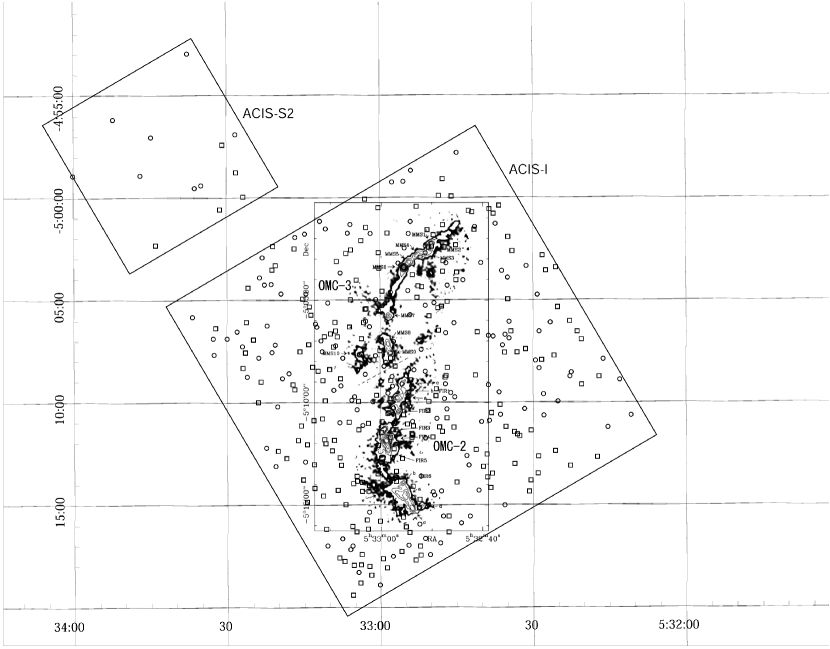
Figure 1: FOVs of ACIS-I (large square region) and ACIS-S2 (small square region at the top left) are overlaid on the 1300mm intensity map (Chini et al., 1997). ACIS-I covers the whole OMC-2 and OMC-3 star forming regions. Squares and circles are X-ray sources with and without a 2MASS counterpart, respectively. The coordinate is in the equinox 1950B.

Figure 1 shows the FOV of our observation overlaid on the 1300mm intensity contour map (Chini et al., 1997). OMC-2 and OMC-3 are separated into south and north by the dotted line. Our observation fully covers both star forming clouds.

3 DATA REDUCTION AND ANALYSIS

3.1 Data Reduction

For the data reduction, we use the level 2 data “reprocessed” at the Chandra X-ray Center (CXC). This version improves the aspect solution and restores the degradation of energy gain and resolution due to the increase of the charge transfer inefficiency (CTI) of the ACIS. For data manipulation, we use the Chandra Interactive Analysis of Observations (CIAO) version 2.1 and FTOOLS version 4.2.

In order to avoid the “spiking” problem reported by the CXC, we manually randomize the values of ENERGY and PI columns in the event file. After this procedure, we conduct the analysis in the following sections separately for the ACIS-I and ACIS-S data. Throughout this paper, we use X-ray photons in the 0.5–8.0 keV energy band. The photons of each source are accumulated from an elliptical region. The major and minor axes, and the rotation angles are derived from the wavdetect command.

3.2 Source Finding

We use wavdetect command with the significance criterion of $1\times 10^{-5}$ and the wavelet scales ranging from 1 to 16 pixels in multiples of $\sqrt{2}$. We remove a few spurious sources through careful inspection by eye. We then detect 365 sources in the 0.5–8.0 keV band image. In order to pick up either soft (less absorbed) or hard (highly absorbed) sources more effectively, we also apply the same detection algorithm to the 0.5–2.0 keV (soft) and 2.0–8.0 keV (hard) band image. Then 17 and 16 new sources are found in the hard band and the soft band image, respectively. In total, we detect 398 X-ray sources in the ACIS-I and ACIS-S FOV. For each detected source, we calculate the X-ray photon count (0.5–8.0 keV) and the hardness ratio (Table 1).

For a systematic study, we divide all the X-ray sources into two groups, “bright” ($>$ 200 counts) and “faint” ($\leq$ 200 counts) sources, according to the photon counts inside the accumulation region. Out of 398 sources, 136 sources are “bright”, and 262 are “faint”. If the X-ray counts of the “bright” sources are less than 3 times the background counts in the photon accumulation region, we remove these sources and define the remaining 123 sources to be “bright2”. This screening is practically necessary to comprise a good sample for spectral and timing analyses. In particular, those at large off-axis angles have the background counts comparable to 200 due to a rather large accumulation area, hence the background has a large impact on the quality of the source spectrum and light curve.

3.3 Correlation with 2MASS Sources

For all the detected X-ray sources, we search for a NIR counterpart using the Point Source Catalog in the 2MASS Second Incremental Data Release. It covers the whole ACIS-I and ACIS-S FOVs, and provides us with the NIR source positions and their photometric data in the J, H, and K_s-band down to 15.8, 15.1, and 14.3 mag, respectively.

In the ACIS-I and ACIS-S FOVs, we find 638 2MASS sources. First, we search for the 2MASS sources nearest to each CXO source within 3^′′ radius. Second, we conversely search for the CXO source nearest to each 2MASS source within 3^′′ radius. Thus we pick up the nearest CXO-2MASS pairs. The systematic position off-sets of the CXO sources from their 2MASS counterparts is found to be $-0\farcs 186$ and $0\farcs 200$ in the direction of right ascension and declination. After correcting these systematic off-sets of the X-ray position, we re-apply the same procedure for the 2MASS counterpart search. Finally we find that 238 out of 398 ($\sim$ 60%) X-ray sources have a 2MASS counterpart. The distance between X-ray sources and their counterparts is found to be $\sim$ 0$\farcs$5.

Together with the X-ray properties, the J–H and H–K colors of their 2MASS counterparts are given in Table 1. About 80% of the “bright” sources have a 2MASS counterpart (111 out of 136), while for the “faint” sources, the ratio is about 50% (127 out of 262).

3.4 Timing Analysis

We make the X-ray light curve (background is not subtracted) for the “bright2” sources and perform $\chi^{2}$ fit with a constant flux assumption. We discriminate the time-variable sources by the significance criteria of 0.01, which are marked with $\dagger$ in Table 2. About 40% (47 out of 123) of the sample sources are found to be time-variable. Most of them show flare-like variability, a fast rise and slow decay of the flux. Some light curves show multiple flares during the observation. A variety of features are seen in the light curves, and it is difficult to separate X-ray photons during the flare and at quiescence in a coherent manner. We therefore deal with them in the same way.

3.5 Spectral Analysis

We next perform spectral analysis of the “bright2” sources, the same data set for the timing analysis. We combine each energy bin so as to have more than 20 photons, then subtract a background spectrum. We use the sherpa program for the spectral fitting.

First we fit the spectrum of all the sample sources with a thin thermal plasma and a power-law model, both with absorption of hydrogen column density ($N_{\rm H}$). The free parameters of the former model are temperature ($k_{B}T$), metallicity ($Z$), and normalization, while the latter’s are photon index ($\Gamma$) and normalization. The former model is accepted for 90 out of 123 sources with the upper probability of larger than 0.01 (99% confidence). The latter model is accepted for 64 sources, of which all except two are also accepted in the former model. On the contrary, both the models are rejected for the other 31 sources. Therefore, here and after, we use the results of the thin-thermal plasma model fittings (Table 2).

Second, for the 31 sources which reject both models, we try 2-component models, 1) a thin-thermal plasma $+$ power-law and 2) 2-temperature thin-thermal plasma model. Additional free parameters are $k_{B}T$ (or $\Gamma$) and normalization. Both models are acceptable for 8 and rejected for 6 sources out of 31 samples, while the latter model are accepted by other 15 sources. We therefore use the results of the two temperature thin-thermal plasma model fittings (Table 3).

4 DISCUSSION

4.1 The Nature of X-ray and NIR Sources

4.1.1 The Nature of NIR Sources

Since some fraction of the 2MASS sources may be background or foreground sources, we first estimate the contribution of background galaxies in the following way. The number counts of galaxies per square degree per magnitude at a certain K-band (2.2µm) magnitude is given by

$$\frac{dN}{dK}=4000\times 10^{\alpha(K-17)}$$ (1)

where $\alpha=0.67$ for 10 mag$<K<$ 17 mag (Tokunaga, 2000). Therefore, the number in the range of $K_{min}$ mag$<K<$ $K_{max}$ mag is

$$\int_{K_{min}}^{K_{max}}\frac{dN}{dK}\ dK=\frac{4000}{\alpha\log{10}}\{10^{\alpha(K_{max}-17)}-10^{\alpha(K_{min}-17)}\}.$$ (2)

The NIR counterparts of the CXO sources have a K-band flux of 6 mag $<K_{s}<$ 15 mag. We substitute $K_{min}=6$ and $K_{max}=15$ for simplicity, though equation (2) is valid only for $K_{min}>$10 mag. Still, this gives us a good estimate, because the second term of the right hand side of equation (2) is negligible compared to the first term in this case. Considering our FOV ($8\farcm 4\times 8\farcm 4$ for each chip), the estimated number of galaxies with 6 mag$<K_{s}<$ 15 mag is $\sim$12. This is only 1.9% of the 2MASS source number in our FOV. In addition, the background galaxies in this direction may suffer significant extinction due to molecular clouds, hence the contribution of extragalactic sources to our 2MASS sources should be even smaller than that estimated above.

We can also neglect the contribution of foreground sources to our 2MASS sample, because OMC-2 and OMC-3 lie off the galactic plane by $\sim$ 20 degrees. Thus, we can safely assume most of the NIR sources to be cloud members (YSOs and MS stars).

4.1.2 The Nature of X-ray Sources

Krishnamurthi et al. (2001) observed the core of the Pleiades star cluster with the CXO for 36 ksec, and found that a significant fraction of X-ray sources are likely to be AGNs. We therefore try to discriminate cloud members from extragalactic sources using the X-ray hardness ratio.

In Figure 2, the histogram of the hardness ratio is given separately for X-ray sources with and without a NIR counterpart. The hardness ratio of the X-ray sources with a NIR counterpart has the peak at $-1.0\sim-0.8$, while those without a NIR counterpart has its peak at $0.2\sim 0.4$. A power-law spectrum of $\Gamma=$1.7 has the hardness ratio of $0.1\sim 0.4$ when absorbed with the column density of $N_{\rm H}$$=$1–2$\times 10^{22}$cm^-2, a typical value of the cloud column density. This corresponds to the peak of X-ray sources without a NIR counterpart. On the contrary, a thin-thermal spectrum with $k_{B}T$$=1.2$ keV, $Z$$=$0.20, and $N_{\rm H}$$=10^{21}$cm^-2, typical values for class III and MS stars (see the following section), has the hardness ratio of $\sim-$0.8. This corresponds to the peak of the histogram of X-ray sources with a NIR counterpart.

Therefore, X-ray sources with a NIR counterpart are mostly cloud members, consistent with the conclusion of the previous subsection. We thus focus on the X-ray sources with a NIR counterpart. X-ray sources without a NIR counterpart, on the other hand, are probably AGNs, which are not the main subject of this paper.

4.2 Classification

YSOs are observationally classified into class 0 through class III based on their spectral energy distribution (SED) from optical, NIR, mid infrared (MIR), and sub-mm bands (André & Montmerle, 1994). Since no systematic catalog for wavelengths longer than MIR is published in both of these clouds, we use the J–H/H–K color-color diagram of the 2MASS counterparts for the classification (Lada & Adams, 1992; Strom, Kepner, & Strom, 1995).

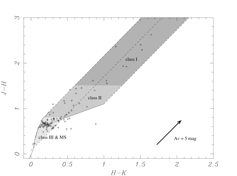
Figure 3: The J–H/H–K color-color diagram in CIT color system. “Bright2” sources with the 2MASS J, H, and K_s-band detection are plotted (crosses). The typical error is $\pm$0.05 mag. The evolution tracks of giants and dwarfs, and CTTS locus are given by solid lines, while the dotted lines represent the extinction vector. X-ray sources are classified into class I, class II, and class III $+$ MS sources based on their position on the diagram.

Out of the 123 “bright2” sources, 108 are detected either in the J, H, or K_s-band, and the remaining 15 are found in none of these bands. Figure 3 shows the J–H vs H–K plots of the detected X-ray sources.

Intrinsic colors for giants and dwarfs are taken from Tokunaga (2000) with colors transformed into the CIT system (Bessel & Brett, 1988), while CTTS locus is taken from Meyer, Calvet, & Hillenbrand (1997). We assume the slope of the reddening lines to be $E(\textit{J--H})/E(\textit{H--K})=1.63$ (Martin & Whittet, 1990). All the 2MASS colors are also translated into CIT color system with the transformation formula established by Carpenter (2001).

Based on the position in this diagram, we classify the sources into three groups — class I, class II, and class III $+$ MS — in the following way. Class I and class II sources are characterized by H–K color excess over J–H color, originating from their disk emission, while class III and MS sources are not. Therefore, sources between the second and the third leftmost reddening lines, and above the CTTS locus are either class I or class II sources. Class I and class II sources in this region can be distinguished from each other by the amount of extinction, where class Is generally have higher extinction (typically J–H$>$1.5) than class IIs (Lada & Adams, 1992; Strom, Kepner, & Strom, 1995). Therefore, sources with J–H$>$1.5 are classified to be class I and J–H$\leq$ 1.5 are class II. Sources between the leftmost and the second leftmost reddening lines can be either class I, class II, class III or MS stars. In this region again, we classify sources based on their amount of extinction; sources with J–H$>$1.5 are class I, J–H$>$0.8 are class II, and J–H$\leq$0.8 are class III $+$ MS. These criteria are based on the fact that, in the Taurus-Auriga dark cloud complex, class II sources rarely have larger extinction than J–H$>$1.5 and class III sources rarely have larger extinction than J–H$>$0.8 (Strom, Kepner, & Strom, 1995). In addition, sources which lack 2MASS J and/or H-band detection (the upper limit of the H-band magnitude is given) are classified as class I, because all of them have larger extinction of H–K$>$1.2 mag.

Then, out of the 108 sources, we find 19 class I, 18 class II, and 61 class III $+$ MS sources. The other 10 are outside of the classification regions. The results are summarized in Table 2.

4.3 X-ray Properties of Different Classes

Based on the classification described in the previous section, we list the X-ray properties (absorption, metallicity, luminosity, and temperature) of each class in Table 4 and compare them with each other.

4.3.1 Absorption

The X-ray absorption decreases as a YSO evolves from class I through class III $+$ MS. This is basically consistent with the fact that we classify these sources using their NIR extinction. J–H derived from the NIR photometry is a good indicator for the amount of material in solid-state, while $N_{\rm H}$ derived from X-ray spectroscopy represents the amount of gas. Therefore, $N_{\rm H}$ should go in proportion to J–H, and the ratio gives us the information of the dust-to-gas ratio in a star forming cloud.

For all the “bright2” sources with NIR data, we plot the relation between $N_{\rm H}$ and J–H (Figure 4). A clear correlation is found. The best-fit linear function is

$$N_{\rm H}/10^{22}~{}\rm{cm}^{-2}=(1.35\pm 0.18)\{(\textit{J--H})-(0.63\pm 0.05)\}\ mag.$$ (3)

The J–H offset of 0.63$\pm$0.05 mag should be the averaged intrinsic color after removing the reddening, which corresponds to the spectral type K5–K7 in MS stars (Tokunaga, 2000). This indicates that low mass YSOs and MS stars are dominant in these clouds. The slope of 1.35$\pm$0.18 gives us information on the dust-to-gas ratio. Together with the relation between $A_{V}$ and J–H given in Meyer et al. (1997),

$$N_{\rm H}/10^{21}~{}\rm{cm}^{-2}=(1.49\pm 0.20)\times A_{V}\ mag$$ (4)

is derived. The slope of 1.49$\pm$0.20 is smaller than those of the Galactic interstellar medium and the $\rho$-Ophiuchi dark cloud, and is similar to that of another star forming region, the Mon R2 cloud (Predehl & Schmitt, 1995; Imanishi et al., 2001; Kohno, Koyama, & Hamaguchi, 2001). Thus the dust-to-gas ratio may scatter from cloud to cloud, possibly with more massive star forming regions having larger dust-to-gas ratio.

4.3.2 Metallicity

We determine the metallicity for many sample stars in a star forming region for the first time. A hint of a decreasing trend toward evolved classes is seen, although this depends on the way the samples are broken into class I, class II, and class III $+$ MS. The metallicity, when all classes are combined, is 0.45 (0.37–0.52) solar.

Padgett (1996) observed 30 G and K pre-main-sequence stars in the nearby star forming regions including Orion, and studied their photospheric abundances using the iron absorption lines in the optical band. All star forming regions are found to have the solar abundance.

The discrepancy between the coronal abundance and the photospheric abundance, which are derived from the X-ray observations and the optical observations respectively, is often seen in other samples Yamauchi et al. (1996); Imanishi et al. (2001).

4.3.3 Luminosity and Temperature

The temperature ($k_{B}T$) and the luminosity ($L_{X}$) are plotted on Figure 5, separately for class I, class II, and class III $+$ MS. The temperatures of class I to class III $+$ MS sources are randomly distributed over a wide range of luminosity, but the mean temperatures of class I and class II sources are significantly higher ($k_{B}T$ $\sim$ 3.0 keV) than that of class III $+$ MS ($k_{B}T$ $\sim$ 1.2 keV). We may argue that there are two types of X-ray emission mechanisms; one exhibits higher temperature, and the other has lower temperature. The former dominates in less evolved YSOs, like class I and class II sources, while the latter gradually appears as YSOs evolve to class III $+$ MS. In this context, it is suggestive that most sources with two temperature components (Table 4) belong to class III $+$ MS. The higher temperature component of these sources has $\sim$ 2.3 keV on average similar to the 1-temperature sources of class I and class II, while the mean of the lower temperature component is $\sim$ 0.8 keV similar to the 1-temperature sources of class III $+$ MS. We hence suspect that the two component class III $+$ MS sources may be in the transition phase between higher-temperature-dominant and the lower-temperature-dominant stage.

4.3.4 Time Variation

Class II sources have a slightly higher fraction of time-variable sources than other classes, though it is not statistically significant. When class I and class II are combined and are compared with class III $+$ MS, we see no significant difference in time-variation rate (in both groups, $\sim$ 40% are time-variable). Imanishi et al. (2001) also argues that no significant difference of the flare rate is seen among three classes in the $\rho$-Ophiuchi dark cloud. Whether time-variable activity is related to the higher-temperature or the lower-temperature-component is not clear in our data set.

5 SUMMARY

We observed OMC-2 and OMC-3 with the CXO/ACIS for $\sim$ 100 ksec. This is one of the deepest observations ever performed in star forming regions in the X-ray band. We detected $\sim$ 400 X-ray sources in our FOV. Coherent analyses on these sources derived the following results.

1. Imaging analysis is performed for all the detected sources, and their position, photon counts, and hardness ratio are derived. This is one of the largest catalogs of X-ray sources in a star forming region.

2. Correlations with the 2MASS sources are found using the 2MASS database. About 60% of the X-ray sources have a NIR counterpart.

3. Spectral and timing analysis are performed for “bright2” X-ray sources. A one temperature thin-thermal plasma model can explain most of the spectra. About 40% of the “bright2” sources are found to be time-variable.

4. Most of the X-ray sources with a NIR counterpart are likely cloud members, while those with no NIR counterpart are probably background AGNs.

5. We classify the cloud members to be class I, class II, and class III $+$ MS based on the J–H/H–K color-color diagram and conduct a systematic comparison on the X-ray properties, such as absorption, luminosity, temperature, and time-variation.

6. Class I and class II sources are found to have higher temperatures than class III $+$ MS. We thus propose that two types of X-ray emission mechanisms exist (higher temperature and lower temperature component). The higher temperature plasma appears in the earlier phase and lower temperature plasma appears as YSOs evolve. In the transition phase, possibly early class III, plasma emissions with different temperatures coexist.

7. The ratio of time-variable sources is nearly the same among different classes. Whether the time-variability is related to higher-temperature- or lower-temperature-plasma is still an open question.

Figure 2: The histogram of the hardness ratio (from –1 to 1 with a step of 0.2) is shown by the dashed and dotted line for the X-ray sources with and without a NIR counterpart, respectively. The total is given by the solid line.

Figure 4: The NIR extinction (J–H mag) and the X-ray absorption ($N_{\rm H}$ 10²²cm^-2) are plotted. The best-fit linear function is expressed with the dashed line.

Figure 5: Luminosity (10²⁹ erg s^-1) in logarithmic scale and temperature (keV) of each source are plotted separately for class I (squares), class II (triangles), and class III $+$ MS (crosses) sources.

Table 1: Results of Imaging Analysis and NIR Identification

ID	Name	X-ray	Hardness	J–H	H–K
		Counts	Ratio	(mag)	(mag)
I1	053438.60-050844.6	255	0.31	$\cdots$	$\cdots$
I2	053440.86-050700.0	63	-0.02	$\cdots$	$\cdots$
I3	053443.10-050919.8	368	0.62	$\cdots$	$\cdots$
I4	053444.89-050650.9	403	-0.54	0.725	0.379
I5	053445.19-051046.9	176	-0.25	0.748	0.517
I6	053448.29-050714.9	535	-0.66	0.658	0.223
I7	053448.37-050502.9	549	-0.77	0.675	0.188
I8	053449.18-050440.0	127	-0.97	0.695	0.227
I9	053450.33-050639.9	70	-0.29	$\cdots$	$\cdots$
I10	053450.43-051113.0	773	-0.75	0.663	0.172
I11	053450.59-050651.6	110	0.40	$\cdots$	$\cdots$
I12	053450.64-050409.4	361	-0.70	0.720	0.289
I13	053453.03-050328.7	1747	-0.73	0.751	0.451
I14	053453.42-051030.0	579	-0.70	0.628	0.232
I15	053453.45-050132.0	49	0.10	0.625	0.210
I16	053453.71-050550.7	145	-0.75	0.644	0.247
I17	053455.38-050141.1	534	-0.83	0.731	0.146
I18	053455.66-050846.1	39	0.38	$\cdots$	$\cdots$
I19	053455.76-050744.3	103	0.24	$\cdots$	$\cdots$
I20	053456.07-050057.4	359	-0.69	0.639	0.213
I21	053456.13-050603.3	276	-0.82	0.613	0.238
I22	053456.64-050627.9	55	0.20	$\cdots$	$\cdots$
I23	053456.67-050439.7	98	0.47	$\cdots$	$\cdots$
I24	053456.71-051045.4	48	-0.33	0.733	0.301
I25	053456.82-051135.3	2286	-0.82	0.713	0.467
I26	053457.35-050605.8	19	0.58	$\cdots$	$\cdots$
I27	053458.19-050929.7	558	-0.71	0.762	0.283
I28	053458.21-051156.4	258	-0.64	0.604	0.219
I29	053458.52-051228.8	135	0.04	0.552	0.236
I30	053459.22-050128.0	28	0.43	$\cdots$	$\cdots$
I31	053459.32-050531.8	740	-0.75	0.767	0.313
I32	053459.47-050827.4	30	0.27	$\cdots$	$\cdots$
I33	053500.40-050946.6	213	0.13	0.567	0.310
I34	053500.87-050941.2	135	-0.72	0.559	0.318
I35	053501.37-051107.9	60	0.33	0.962	0.575
I36	053501.43-050934.6	670	-0.85	0.668	0.180
I37	053501.98-050045.0	63	-0.46	0.631	0.219
I38	053502.16-050440.3	83	-0.76	0.757	0.374
I39	053502.52-050411.8	11	0.82	$\cdots$	$\cdots$
I40	053502.56-050500.3	9	1.00	$\cdots$	$\cdots$
I41	053502.79-050305.7	20	-0.40	0.576	-0.065
I42	053502.79-050003.7	1023	-0.57	1.166	0.453
I43	053502.85-050202.4	20	0.50	$\cdots$	$\cdots$
I44	053503.12-050919.1	90	-0.76	0.718	0.335
I45	053503.30-050449.9	26	0.69	$\cdots$	$\cdots$
I46	053503.33-051308.9	159	0.17	$\cdots$	$\cdots$
I47	053503.41-050542.2	1771	-0.62	0.216	0.027
I48	053503.81-050520.9	17	0.53	$\cdots$	$\cdots$
I49	053503.99-050142.9	20	0.70	$\cdots$	$\cdots$
I50	053504.23-050844.3	54	0.26	$\cdots$	$\cdots$
I51	053504.30-050814.7	25402	-0.55	0.656	0.153
I52	053504.45-050738.3	14	-0.43	$\cdots$	$\cdots$
I53	053504.55-045831.7	109	-0.21	1.055	0.743
I54	053504.64-050957.9	437	-0.78	0.647	0.257
I55	053505.24-045925.0	26	0.54	$\cdots$	$\cdots$
I56	053505.65-045855.4	334	-0.83	0.649	0.236
I57	053505.66-050455.2	7	0.43	$\cdots$	$\cdots$
I58	053505.76-051136.3	92	-0.28	1.394	0.658
I59	053505.95-050839.3	18	-0.67	1.084	0.496
I60	053506.09-051218.8	43	-0.30	-0.077	-0.023
I61	053506.36-050901.8	10	0.20	$\cdots$	$\cdots$
I62	053506.49-045842.2	58	-0.45	0.556	0.301
I63	053506.58-050717.8	15	0.60	$\cdots$	$\cdots$
I64	053506.61-050453.0	42	0.43	$\cdots$	$\cdots$
I65	053506.71-051147.2	257	-0.19	1.439	0.618
I66	053506.83-051040.9	200	-0.76	0.671	0.236
I67	053507.54-051116.5	1232	-0.21	1.066	0.584
I68	053508.04-050120.0	14	0.14	$\cdots$	$\cdots$
I69	053508.75-050442.3	26	-0.85	0.742	0.356
I70	053508.96-051027.4	12	-0.67	0.615	0.095
I71	053509.15-050648.9	1192	-0.83	0.672	0.206
I72	053509.32-045934.0	56	0.39	$\cdots$	$\cdots$
I73	053509.42-045943.0	72	-0.56	0.680	0.348
I74	053509.85-045850.9	442	0.24	$\cdots$	1.612
I75	053510.14-051342.4	86	0.00	$\cdots$	$\cdots$
I76	053510.32-051112.9	13	0.54	$\cdots$	$\cdots$
I77	053510.51-045847.3	835	0.52	$\cdots$	3.286
I78	053511.56-050210.0	16	0.75	$\cdots$	$\cdots$
I79	053511.81-051401.8	237	-0.09	$\cdots$	$\cdots$
I80	053512.72-051202.6	59	-0.46	0.524	0.250
I81	053512.80-050147.9	79	-0.95	0.590	0.279
I82	053512.92-045557.4	325	0.48	$\cdots$	$\cdots$
I83	053512.95-050210.3	109	-0.83	0.558	0.328
I84	053513.00-050028.0	29	0.38	$\cdots$	$\cdots$
I85	053513.34-050921.7	1088	-0.74	0.683	0.189
I86	053513.35-050416.3	7	0.71	$\cdots$	$\cdots$
I87	053513.88-045805.0	207	0.11	2.364	1.164
I88	053513.99-050740.6	21	0.81	$\cdots$	$\cdots$
I89	053514.28-051428.1	268	0.01	2.401	1.504
I90	053514.29-051342.1	116	0.00	1.941	1.264
I91	053514.63-050627.1	34	-0.65	1.156	0.653
I92	053514.64-050226.5	312	-0.82	$\cdots$	$\cdots$
I93	053514.66-050314.2	574	-0.85	0.676	0.183
I94	053514.67-050854.1	33	-0.76	0.572	0.282
I95	053514.70-050828.0	4	1.00	$\cdots$	$\cdots$
I96	053514.87-050650.6	333	0.16	$\cdots$	1.216
I97	053514.94-050120.1	24	0.58	$\cdots$	$\cdots$
I98	053514.99-050715.0	62	0.71	$\cdots$	$\cdots$
I99	053515.08-050655.4	112	0.21	2.294	1.198
I100	053515.18-050758.2	4	0.50	$\cdots$	$\cdots$
I101	053515.27-050034.4	29	-0.86	0.631	0.256
I102	053515.36-051342.0	68	-0.53	$\cdots$	$\cdots$
I103	053515.49-050114.0	26	-0.31	0.677	0.337
I104	053515.55-050145.3	34	-0.53	1.093	0.525
I105	053515.59-050934.0	21	-0.33	0.590	0.277
I106	053515.61-045929.1	151	-0.30	1.899	1.092
I107	053515.65-045714.5	159	-0.47	0.767	0.315
I108	053515.76-051229.2	72	0.06	$\cdots$	$\cdots$
I109	053515.80-050327.8	177	-0.92	0.579	0.339
I110	053515.93-051501.3	3013	0.20	$\cdots$	$\cdots$
I111	053516.14-050921.1	88	-0.91	0.622	0.234
I112	053516.35-050438.1	17	-0.76	0.561	0.329
I113	053516.40-045803.7	264	-0.79	0.605	0.161
I114	053516.49-050332.0	294	-0.80	0.655	0.197
I115	053516.66-050856.2	4	0.50	$\cdots$	$\cdots$
I116	053516.80-050729.2	45	-0.91	0.490	0.341
I117	053516.86-050749.5	16	-0.62	0.995	0.540
I118	053517.12-051240.9	74	-0.54	$\cdots$	$\cdots$
I119	053517.25-050317.7	10	0.80	$\cdots$	$\cdots$
I120	053517.36-051231.1	65	-0.66	$\cdots$	$\cdots$
I121	053517.41-045958.4	259	0.20	$\cdots$	1.775
I122	053517.46-050950.9	44	-1.00	0.578	0.299
I123	053517.72-050032.1	29	-0.17	2.217	1.373
I124	053517.92-051535.0	830	-0.14	$\cdots$	$\cdots$
I125	053518.24-051308.9	561	-0.40	$\cdots$	$\cdots$
I126	053518.24-050355.9	92	-1.00	0.041	0.013
I127	053518.26-050806.9	7	-0.14	$\cdots$	1.263
I128	053518.31-050034.8	60	0.93	$\cdots$	$\cdots$
I129	053518.45-050832.7	15	-0.73	0.595	0.235
I130	053518.61-045944.0	165	-0.71	0.583	0.201
I131	053518.84-051448.1	661	-0.48	$\cdots$	$\cdots$
I132	053518.93-050051.9	23	0.65	$\cdots$	$\cdots$
I133	053518.94-050638.1	26	0.85	$\cdots$	$\cdots$
I134	053518.96-050324.9	7	1.00	$\cdots$	$\cdots$
I135	053518.98-050031.0	24	0.83	$\cdots$	$\cdots$
I136	053519.65-050230.4	11	-0.82	0.647	0.307
I137	053519.75-050533.4	6	0.67	$\cdots$	$\cdots$
I138	053519.75-051536.7	359	0.67	$\cdots$	$\cdots$
I139	053519.86-051510.2	309	0.25	1.610	1.034
I140	053519.97-050104.1	259	0.83	$\cdots$	$\cdots$
I141	053519.98-051405.6	202	0.03	$\cdots$	$\cdots$
I142	053519.99-051252.9	97	0.86	2.063	1.310
I143	053520.08-051318.8	1099	0.06	$\cdots$	$\cdots$
I144	053520.14-051317.3	953	0.05	1.923	1.308
I145	053520.37-050228.2	73	-0.86	0.765	0.203
I146	053520.59-050302.0	7	0.43	$\cdots$	2.444
I147	053520.74-051551.3	2276	-0.12	1.177	0.558
I148	053520.76-045835.6	673	-0.37	1.118	0.463
I149	053521.13-050634.2	109	0.63	$\cdots$	$\cdots$
I150	053521.26-050918.2	2202	-0.81	0.547	0.489
I151	053521.31-051214.9	14667	-0.63	0.604	0.176
I152	053521.39-050944.2	29	-0.79	0.686	0.490
I153	053521.44-050905.6	142	-0.62	$\cdots$	$\cdots$
I154	053521.50-050155.3	97	0.13	$\cdots$	2.056
I155	053521.56-050941.0	76	0.84	0.837	0.715
I156	053521.57-050951.7	260	-0.64	0.784	0.528
I157	053521.86-045650.5	93	0.08	$\cdots$	$\cdots$
I158	053521.87-050703.7	838	-0.71	0.950	0.558
I159	053521.91-045919.5	15	-0.20	$\cdots$	$\cdots$
I160	053521.92-050352.4	8	0.25	$\cdots$	$\cdots$
I161	053521.94-051430.1	345	-0.69	0.747	0.226
I162	053522.11-051507.7	479	-0.32	$\cdots$	$\cdots$
I163	053522.34-045954.7	23	0.65	$\cdots$	$\cdots$
I164	053522.35-050741.0	507	0.02	2.624	1.649
I165	053522.40-050807.0	833	0.21	1.396	0.873
I166	053522.45-050913.0	415	-0.92	0.583	0.124
I167	053522.55-050802.6	921	-0.34	1.412	0.531
I168	053522.67-051413.8	206	-0.69	0.903	0.519
I169	053523.13-050037.7	13	-0.08	$\cdots$	$\cdots$
I170	053523.20-051345.6	164	0.04	1.756	0.742
I171	053523.22-050845.8	13	-0.38	$\cdots$	1.935
I172	053523.33-045722.3	182	-0.63	$\cdots$	$\cdots$
I173	053523.33-050823.5	59	0.19	$\cdots$	2.256
I174	053523.44-051053.9	1909	-0.82	0.628	0.250
I175	053523.51-050715.6	33	0.76	$\cdots$	$\cdots$
I176	053523.53-051525.9	96	-0.25	$\cdots$	$\cdots$
I177	053524.34-050122.2	277	0.58	$\cdots$	$\cdots$
I178	053524.58-051131.5	83	-0.25	1.231	0.672
I179	053524.61-051200.7	363	-0.81	0.767	0.505
I180	053524.66-050929.4	9	0.56	$\cdots$	1.670
I181	053524.87-050623.1	144	0.68	2.994	1.855
I182	053525.03-050911.4	26	-0.85	0.629	0.321
I183	053525.07-051025.3	22	0.82	1.963	1.867
I184	053525.17-050510.9	12	0.00	$\cdots$	$\cdots$
I185	053525.17-051540.6	162	-0.06	$\cdots$	$\cdots$
I186	053525.22-050825.6	66	0.94	$\cdots$	$\cdots$
I187	053525.24-050929.4	544	-0.86	0.689	0.227
I188	053525.36-050722.1	4	0.50	$\cdots$	$\cdots$
I189	053525.40-051050.1	762	-0.83	0.600	0.128
I190	053525.44-050654.1	6	1.00	$\cdots$	$\cdots$
I191	053525.53-045724.6	145	0.10	$\cdots$	$\cdots$
I192	053525.64-050759.2	324	-0.64	0.659	0.888
I193	053525.72-050705.2	5	-1.00	0.646	0.283
I194	053525.73-050951.5	1411	-0.68	0.615	0.335
I195	053525.77-050559.7	9	0.11	$\cdots$	$\cdots$
I196	053525.85-050247.0	5	1.00	$\cdots$	$\cdots$
I197	053525.86-050758.3	878	-0.79	1.027	$\cdots$
I198	053526.05-050839.7	83	-0.76	0.586	$\cdots$
I199	053526.27-050742.9	8	1.00	$\cdots$	$\cdots$
I200	053526.29-050841.9	3840	-0.84	0.504	0.224
I201	053526.34-051613.8	231	-0.06	1.455	0.764
I202	053526.47-045953.8	88	0.20	$\cdots$	1.206
I203	053526.66-050611.9	11	1.00	$\cdots$	$\cdots$
I204	053526.85-051109.7	289	0.13	1.039	0.766
I205	053527.07-050623.5	12	0.67	$\cdots$	$\cdots$
I206	053527.15-051547.1	196	-0.08	0.887	0.512
I207	053527.41-050905.8	18	-0.89	0.768	0.453
I208	053527.45-050243.9	270	0.16	$\cdots$	2.101
I209	053527.63-050938.6	24	0.42	2.435	1.499
I210	053527.73-051357.4	55	0.60	1.285	0.657
I211	053527.79-051704.7	711	-0.46	$\cdots$	$\cdots$
I212	053527.83-050537.9	345	0.57	$\cdots$	$\cdots$
I213	053528.06-050136.6	326	0.42	$\cdots$	2.365
I214	053528.14-051015.3	37	-0.41	0.997	0.662
I215	053528.18-050342.7	41	0.41	$\cdots$	$\cdots$
I216	053528.19-050051.0	172	-0.79	0.651	0.221
I217	053528.21-051139.0	50	-0.28	1.059	0.515
I218	053528.27-045839.8	1228	0.61	$\cdots$	2.812
I219	053528.50-050748.6	89	0.03	$\cdots$	2.158
I220	053528.60-050546.0	28	0.29	2.581	1.501
I221	053528.67-050307.9	8	0.50	$\cdots$	$\cdots$
I222	053528.71-050553.0	11	0.82	$\cdots$	$\cdots$
I223	053529.02-050605.6	1424	-0.82	0.582	0.171
I224	053529.25-050807.1	6	0.67	$\cdots$	$\cdots$
I225	053529.45-051635.3	1189	-0.53	0.864	0.257
I226	053529.81-051609.4	476	-0.63	0.780	0.311
I227	053529.89-051212.4	136	-0.78	0.646	0.200
I228	053529.90-050428.5	8	1.00	$\cdots$	$\cdots$
I229	053530.00-051229.5	157	-0.61	0.705	0.487
I230	053530.11-050911.3	23	-0.74	0.602	0.266
I231	053530.13-051420.8	148	-0.27	1.180	0.607
I232	053530.32-051353.8	213	-0.10	1.612	0.849
I233	053530.55-050335.7	13	-0.08	$\cdots$	$\cdots$
I234	053530.64-045937.4	222	-0.34	2.291	1.522
I235	053530.72-050647.1	6	0.33	$\cdots$	$\cdots$
I236	053530.86-045814.2	67	0.25	$\cdots$	1.693
I237	053531.06-050416.0	91	-0.93	0.571	0.115
I238	053531.22-051230.1	311	-0.80	0.660	0.231
I239	053531.27-051203.6	82	-0.41	0.620	0.299
I240	053531.31-051535.1	2773	-0.64	0.777	0.315
I241	053531.46-050547.3	22	0.91	$\cdots$	$\cdots$
I242	053531.48-051605.0	660	-0.78	0.226	0.050
I243	053531.49-050503.2	187	-0.80	0.688	0.477
I244	053531.57-050548.9	13	0.85	2.003	1.424
I245	053531.58-051658.2	181	-0.28	1.168	0.504
I246	053531.61-050015.8	63	0.49	2.628	1.639
I247	053531.91-050551.1	33	0.39	$\cdots$	$\cdots$
I248	053531.96-050929.7	2062	-0.65	0.812	0.414
I249	053532.02-050807.0	7	-0.14	1.046	0.618
I250	053532.24-051200.1	38	-0.53	0.746	0.484
I251	053532.31-051145.8	175	0.29	2.176	1.141
I252	053532.35-051428.1	150	-0.45	0.982	0.356
I253	053532.35-050831.6	25	0.76	$\cdots$	$\cdots$
I254	053532.51-050211.7	14	-0.71	0.599	0.193
I255	053532.80-050753.4	23	0.65	$\cdots$	$\cdots$
I256	053532.86-051606.4	1143	-0.39	1.093	0.302
I257	053532.97-051207.7	25	0.12	2.036	1.154
I258	053533.00-051734.1	406	-0.63	0.619	0.271
I259	053533.16-051412.9	974	-0.14	0.783	0.399
I260	053533.38-050803.8	11	0.82	$\cdots$	$\cdots$
I261	053533.52-051521.1	646	-0.11	$\cdots$	$\cdots$
I262	053533.61-050043.5	128	-0.83	0.652	0.200
I263	053533.64-050309.5	223	-0.35	1.451	0.693
I264	053533.83-050429.0	346	0.88	1.934	1.264
I265	053533.86-050907.4	20	-0.80	0.586	0.264
I266	053534.26-045954.5	53	0.89	$\cdots$	$\cdots$
I267	053534.48-051309.1	76	-0.61	0.583	0.161
I268	053534.52-050053.6	27	0.48	2.309	2.173
I269	053534.68-051555.1	330	-0.67	0.556	0.550
I270	053535.11-051449.0	99	0.33	$\cdots$	$\cdots$
I271	053535.12-050600.0	13	1.00	$\cdots$	$\cdots$
I272	053535.36-051113.6	506	-0.72	0.577	0.217
I273	053535.48-050722.0	27	0.93	$\cdots$	$\cdots$
I274	053535.55-050700.3	210	-0.90	0.628	0.208
I275	053535.63-050150.3	66	0.91	$\cdots$	$\cdots$
I276	053535.64-051051.8	22	-0.55	0.517	0.351
I277	053535.71-051545.1	204	-0.26	0.678	0.284
I278	053536.02-051226.9	270	-0.61	1.551	1.042
I279	053536.19-050457.6	114	0.60	1.349	0.722
I280	053536.40-050117.0	943	-0.46	0.836	0.467
I281	053536.51-050524.1	9	0.33	$\cdots$	$\cdots$
I282	053536.56-050440.9	909	-0.92	0.654	0.193
I283	053536.69-050415.8	2221	-0.67	0.746	0.315
I284	053536.77-051000.9	11	-0.45	0.796	0.557
I285	053536.86-050734.2	10	0.60	$\cdots$	$\cdots$
I286	053536.95-050527.6	24	-0.33	0.508	0.432
I287	053537.17-051031.4	312	-0.88	0.677	0.268
I288	053537.57-050449.2	16	0.12	$\cdots$	1.505
I289	053537.70-050633.6	298	-0.64	0.668	0.283
I290	053538.04-051510.1	122	0.48	$\cdots$	$\cdots$
I291	053538.07-050318.9	13	0.38	$\cdots$	$\cdots$
I292	053538.30-051420.9	246	-0.42	0.750	0.223
I293	053538.52-045942.0	518	-0.31	$\cdots$	$\cdots$
I294	053538.57-050805.2	75	0.12	2.532	1.365
I295	053538.65-050958.6	320	-0.72	0.578	0.303
I296	053538.75-050457.1	40	-0.55	1.936	1.035
I297	053538.88-051244.0	1047	-0.26	1.110	0.661
I298	053539.04-050705.8	279	-0.84	0.559	0.291
I299	053539.08-050858.2	198	-0.80	0.664	0.163
I300	053539.17-050541.8	7	0.14	$\cdots$	$\cdots$
I301	053539.39-050509.5	113	0.59	$\cdots$	$\cdots$
I302	053539.72-045920.2	65	0.35	$\cdots$	$\cdots$
I303	053539.97-050638.3	75	-0.68	1.134	0.606
I304	053540.19-050429.1	9	0.33	$\cdots$	$\cdots$
I305	053540.47-050420.5	19	0.58	$\cdots$	$\cdots$
I306	053540.59-051221.6	85	-0.13	0.690	0.270
I307	053540.66-051111.8	76	0.11	0.654	0.289
I308	053540.80-050902.9	825	-0.61	0.903	0.305
I309	053541.04-050626.7	119	-0.76	0.619	0.302
I310	053541.38-050354.4	38	-0.58	1.173	0.491
I311	053541.72-050330.1	61	-0.74	0.612	0.198
I312	053541.81-050520.9	15	-0.33	1.702	0.827
I313	053542.04-051013.8	660	-0.32	1.329	0.617
I314	053542.04-051301.8	617	-0.73	0.559	0.288
I315	053542.40-051104.3	56	0.32	$\cdots$	$\cdots$
I316	053542.64-045957.2	79	0.34	$\cdots$	$\cdots$
I317	053542.78-051156.9	658	-0.79	0.704	0.158
I318	053542.98-050307.1	42	-0.33	0.644	0.274
I319	053543.27-050918.6	2262	-0.79	0.682	0.169
I320	053543.54-050542.0	48	-0.08	0.874	0.689
I321	053543.82-051001.6	174	-0.67	0.597	0.268
I322	053544.52-050733.2	288	-0.87	0.705	0.200
I323	053544.54-050006.7	45	0.24	$\cdots$	$\cdots$
I324	053544.88-050718.5	5273	-0.70	0.630	0.247
I325	053545.70-050646.5	74	0.51	$\cdots$	$\cdots$
I326	053546.10-051054.2	695	-0.76	0.776	0.407
I327	053547.25-050251.9	64	0.41	$\cdots$	$\cdots$
I328	053547.77-051033.0	3604	-0.81	0.542	0.212
I329	053548.26-051117.3	60	0.07	$\cdots$	$\cdots$
I330	053548.39-050522.4	67	0.55	$\cdots$	$\cdots$
I331	053548.40-050129.7	193	-0.60	0.928	0.680
I332	053548.88-050033.4	88	-0.45	0.968	0.271
I333	053549.00-050544.0	31	0.10	$\cdots$	$\cdots$
I334	053549.04-050142.4	288	-0.49	0.771	0.355
I335	053549.21-050225.0	49	0.55	$\cdots$	$\cdots$
I336	053549.96-050426.2	88	0.39	$\cdots$	$\cdots$
I337	053550.07-051024.0	63	-0.33	$\cdots$	$\cdots$
I338	053550.51-050226.5	63	0.27	$\cdots$	$\cdots$
I339	053551.12-050710.5	1348	-0.78	0.736	0.372
I340	053551.46-050205.5	167	0.46	$\cdots$	$\cdots$
I341	053551.61-050600.5	48	0.25	$\cdots$	$\cdots$
I342	053551.66-050810.8	7972	-0.73	0.625	0.143
I343	053552.66-050507.0	4600	-0.75	0.579	0.373
I344	053553.71-050235.6	164	-0.07	1.037	0.347
I345	053553.86-050656.1	258	0.34	$\cdots$	$\cdots$
I346	053554.05-050416.3	1398	-0.81	0.867	0.489
I347	053554.22-050545.0	74	-0.03	0.654	0.204
I348	053554.67-050630.3	168	-0.56	0.554	0.301
I349	053555.86-050444.3	87	0.24	$\cdots$	$\cdots$
I350	053557.79-050504.6	169	0.14	$\cdots$	$\cdots$
I351	053600.05-050434.0	134	-0.27	0.574	0.406
I352	053600.36-050552.3	68	0.06	$\cdots$	$\cdots$
I353	053600.55-050505.3	413	-0.27	$\cdots$	$\cdots$
I354	053604.60-050402.3	250	0.10	$\cdots$	$\cdots$
I355	053454.47-050414.3	18	0.67	$\cdots$	$\cdots$
I356	053457.03-050252.0	6	1.00	$\cdots$	$\cdots$
I357	053508.43-051226.3	34	0.47	$\cdots$	$\cdots$
I358	053513.13-050753.3	4	1.00	$\cdots$	$\cdots$
I359	053518.87-050953.2	5	1.00	$\cdots$	$\cdots$
I360	053521.33-051248.1	15	0.47	$\cdots$	$\cdots$
I361	053521.50-050727.8	4	1.00	$\cdots$	$\cdots$
I362	053522.42-050242.4	4	1.00	$\cdots$	$\cdots$
I363	053522.67-050651.3	3	1.00	$\cdots$	$\cdots$
I364	053529.78-045955.7	27	0.63	$\cdots$	$\cdots$
I365	053530.67-050411.7	4	1.00	$\cdots$	$\cdots$
I366	053531.19-050917.5	8	1.00	$\cdots$	$\cdots$
I367	053533.14-051510.5	268	0.26	$\cdots$	$\cdots$
I368	053547.84-050823.3	28	0.57	$\cdots$	$\cdots$
I369	053550.91-050106.7	91	0.45	$\cdots$	$\cdots$
I370	053444.08-050600.1	57	0.30	$\cdots$	$\cdots$
I371	053452.91-050805.0	18	0.00	$\cdots$	$\cdots$
I372	053500.97-050541.4	8	-0.75	0.410	0.346
I373	053507.89-050905.3	3	-1.00	$\cdots$	$\cdots$
I374	053510.79-051045.3	3	-1.00	$\cdots$	$\cdots$
I375	053514.97-050444.9	3	-1.00	$\cdots$	$\cdots$
I376	053519.73-051145.3	34	0.00	$\cdots$	$\cdots$
I377	053529.82-051330.9	49	0.18	$\cdots$	$\cdots$
I378	053530.76-050337.3	5	-1.00	$\cdots$	$\cdots$
I379	053533.75-045928.7	15	-0.07	$\cdots$	$\cdots$
I380	053535.70-050909.1	6	-0.33	$\cdots$	$\cdots$
I381	053538.44-051010.5	28	-0.50	0.608	0.314
I382	053542.37-050252.1	15	-0.60	$\cdots$	$\cdots$
I383	053544.67-050040.4	31	-0.55	0.754	0.347
I384	053546.94-050700.7	14	-0.29	$\cdots$	$\cdots$
I385	053554.84-050527.6	23	-0.30	$\cdots$	$\cdots$
S1	053554.73-045808.9	2987	-0.87	0.483	0.168
S2	053556.14-045657.7	1681	-0.75	0.616	0.189
S3	053556.28-045505.9	510	0.13	$\cdots$	$\cdots$
S4	053558.84-045537.0	799	0.03	$\cdots$	0.808
S5	053559.31-045846.1	743	-0.64	0.695	0.162
S6	053602.99-045736.2	304	-0.30	$\cdots$	$\cdots$
S7	053604.24-045744.3	285	-0.25	$\cdots$	$\cdots$
S8	053605.75-045110.3	832	-0.39	$\cdots$	$\cdots$
S9	053611.84-050032.2	567	-0.47	0.690	0.168
S10	053612.81-045515.5	462	-0.29	$\cdots$	$\cdots$
S11	053628.11-045709.3	185	0.43	$\cdots$	$\cdots$
S12	053614.94-045707.7	72	0.47	$\cdots$	$\cdots$
S13	053620.26-045424.0	164	0.34	$\cdots$	$\cdots$

Table 2: Results of Timing and Spectroscopic Analysis

ID	Upper	$N_{\rm H}$	$k_{B}T$	Metallicity	$L_{X}$	Class
	Probability	($10^{22}$ cm-2)	(keV)	(solar)	(1029 erg s-1)
I4†	0.005	0.14 (0.12–0.16)	1.40 (1.29–1.60)	0.10 (0.07–0.12)	6.90 (6.50–7.31)	III$+$MS
I6†	0.000	0.07 (0.05–0.08)	0.99 (0.94–1.04)	0.10 (0.09–0.12)	7.64 (7.28–8.01)	III$+$MS
I7	0.014	0.14 (0.13–0.16)	0.85 (0.81–0.88)	0.07 (0.06–0.08)	9.95 (9.50–10.41)	III$+$MS
I10	0.008	0.07 (0.05–0.08)	0.98 (0.94–1.02)	0.13 (0.12–0.14)	11.51 (11.07–11.96)	III$+$MS
I12	0.196	0.14 (0.12–0.16)	1.25 (1.16–1.34)	0.13 (0.11–0.15)	6.62 (6.24–6.99)	III$+$MS
I13†	0.000	0.07 (0.06–0.07)	1.09 (1.06–1.13)	0.03 (0.02–0.03)	27.49 (26.78–28.19)	other
I14	0.079	0.02 (0.01–0.04)	1.11 (1.06–1.34)	0.08 (0.07–0.10)	8.14 (7.78–8.50)	III$+$MS
I17	0.245	0.05 (0.04–0.07)	1.02 (0.96–1.07)	0.07 (0.06–0.08)	8.28 (7.91–8.66)	III$+$MS
I20†	0.000	0.12 (0.10–0.14)	0.80 (0.76–0.84)	0.12 (0.10–0.13)	5.37 (5.04–5.69)	III$+$MS
I21	0.226	0.00 (0.00–0.01)	1.06 (1.00–1.12)	0.14 (0.12–0.16)	3.56 (3.34–3.78)	III$+$MS
I25†	0.013	0.05 (0.05–0.06)	1.05 (1.02–1.07)	0.14 (0.13–0.15)	35.16 (34.41–35.92)	other
I27	0.266	0.17 (0.16–0.19)	1.31 (1.25–1.37)	0.26 (0.24–0.29)	10.69 (10.22–11.17)	III$+$MS
I28	0.015	0.00 (0.00–0.02)	1.26 (1.14–1.38)	0.16 (0.13–0.19)	3.10 (2.88–3.32)	III$+$MS
I31	0.110	0.32 (0.30–0.34)	1.03 (1.00–1.07)	0.12 (0.11–0.14)	18.72 (18.01–19.43)	III$+$MS
I33	0.000	0.14 (0.11–0.18)	0.85 (0.76–0.96)	0.07 (0.05–0.09)	1.90 (1.70–2.10)	III$+$MS
I36	0.124	0.03 (0.02–0.05)	1.21 (1.16–1.26)	0.36 (0.34–0.39)	9.15 (8.79–9.51)	III$+$MS
I42†	0.006	0.34 (0.33–0.36)	1.63 (1.55–1.71)	0.16 (0.14–0.18)	28.50 (27.57–29.43)	II
I47†	0.001	0.29 (0.28–0.31)	1.65 (1.59–1.71)	0.19 (0.17–0.21)	43.22 (42.16–44.28)	III$+$MS
I51	0.000	0.19 (0.18–0.19)	2.56 (2.52–2.59)	0.38 (0.37–0.39)	612.99 (609.09–616.87)	III$+$MS
I54	0.603	0.10 (0.08–0.12)	1.22 (1.14–1.29)	0.23 (0.21–0.26)	7.16 (6.81–7.51)	III$+$MS
I56	0.058	0.06 (0.05–0.08)	0.74 (0.69–0.79)	0.11 (0.10–0.12)	4.97 (4.68–5.26)	III$+$MS
I65†	0.665	0.53 (0.48–0.59)	3.35 (2.91–3.83)	0.00 (-0.16–0.14)	10.13 (9.44–10.81)	II
I67†	0.813	0.88 (0.85–0.91)	2.95 (2.83–3.14)	1.60 (1.50–1.71)	64.39 (62.53–66.26)	II
I71	0.001	0.00 (0.00–0.03)	1.04 (1.02–1.07)	0.20 (0.19–0.21)	14.26 (13.84–14.69)	III$+$MS
I74	0.691	2.16 (2.07–2.25)	2.31 (2.19–2.46)	0.28 (0.18–0.37)	45.76 (43.47–48.02)	I
I77	0.240	3.31 (3.21–3.41)	2.91 (2.79–3.07)	0.74 (0.65–0.85)	116.03 (111.84–120.22)	I
I82	0.177	3.92 (3.70–4.16)	2.24 (2.01–2.56)	4.03 (3.60–4.46)	49.90 (46.16–53.67)	$\cdots$
I85†	0.026	0.01 (0.00–0.03)	1.63 (1.55–1.70)	0.35 (0.32–0.38)	33.26 (32.23–34.31)	III$+$MS
I87	0.788	2.57 (2.44–2.72)	1.68 (1.53–1.83)	2.44 (2.17–2.71)	32.89 (30.30–35.48)	I
I89	0.000	1.01 (0.89–1.15)	7.05 (4.97–12.32)	0.26 (-0.20–0.72)	11.65 (10.59–12.71)	I
I92	0.193	0.07 (0.05–0.09)	0.98 (0.92–1.05)	0.15 (0.13–0.17)	4.48 (4.22–4.75)	$\cdots$
I93†	0.856	0.07 (0.05–0.08)	0.84 (0.81–0.88)	0.07 (0.07–0.08)	8.54 (8.17–8.90)	III$+$MS
I96	0.262	1.90 (1.81–2.00)	2.46 (2.31–2.61)	0.01 (-0.09–0.11)	28.04 (26.46–29.62)	I
I110†	0.849	1.21 (1.18–1.24)	7.61 (7.13–8.37)	0.11 (0.03–0.19)	209.63 (205.71–213.57)	$\cdots$
I113	0.512	0.00 (0.00–0.03)	0.82 (0.77–0.87)	0.12 (0.11–0.14)	3.28 (3.06–3.50)	III$+$MS
I114	0.124	0.08 (0.06–0.10)	0.82 (0.78–0.87)	0.23 (0.21–0.25)	4.09 (3.84–4.33)	III$+$MS
I121	0.981	2.47 (2.36–2.60)	1.93 (1.77–2.10)	1.06 (0.92–1.21)	34.47 (32.28–36.66)	I
I124†	0.930	0.74 (0.71–0.79)	3.52 (3.23–3.70)	0.00 (-0.16–0.04)	41.27 (39.16–42.37)	$\cdots$
I125	0.430	0.54 (0.51–0.58)	2.56 (2.33–2.79)	0.62 (0.53–0.72)	20.92 (19.99–21.85)	$\cdots$
I131†	0.461	0.23 (0.21–0.25)	2.83 (2.56–3.18)	0.25 (0.17–0.33)	17.72 (16.98–18.48)	$\cdots$
I138†	0.441	3.60 (3.41–3.82)	5.23 (4.65–5.84)	0.00 (-0.25–0.24)	48.11 (45.34–50.89)	I
I139	0.000	0.00 (0.00–0.00)	3.56 (3.45–3.56)	0.32 (-0.40–0.44)	2.06 (1.82–2.30)	I
I140	0.400	5.88 (5.56–6.23)	3.22 (2.92–3.52)	1.20 (0.95–1.45)	60.02 (56.14–63.90)	I
I141	0.041	0.33 (0.26–0.42)	5.55 (3.71–9.64)	0.55 (0.07–1.03)	4.78 (4.27–5.29)	$\cdots$
I143	0.352	1.68 (1.63–1.73)	2.62 (2.50–2.74)	0.44 (0.37–0.51)	89.11 (86.28–91.92)	$\cdots$
I144	0.363	1.51 (1.46–1.56)	2.73 (2.62–2.84)	0.00 (-0.06–0.07)	70.64 (68.28–73.04)	I
I147†	0.051	1.07 (1.05–1.10)	2.66 (2.57–2.75)	0.26 (0.22–0.30)	138.00 (134.98–141.05)	II
I148†	0.083	0.59 (0.56–0.62)	2.39 (2.23–2.56)	0.09 (0.04–0.15)	26.85 (25.76–27.94)	II
I150†	0.000	0.21 (0.20–0.22)	0.95 (0.93–0.97)	0.23 (0.22–0.24)	42.64 (41.71–43.58)	other
I151	0.000	0.32 (0.32–0.32)	1.67 (1.65–1.69)	0.33 (0.32–0.34)	395.08 (391.75–398.37)	III$+$MS
I156	0.005	0.08 (0.05–0.11)	3.17 (2.74–3.67)	1.63 (1.39–1.88)	5.55 (5.18–5.91)	other
I158	0.256	0.27 (0.25–0.29)	1.33 (1.28–1.39)	0.22 (0.20–0.24)	18.63 (17.97–19.28)	II
I161	0.195	0.12 (0.10–0.15)	0.94 (0.88–1.00)	0.14 (0.13–0.16)	5.54 (5.20–5.87)	III$+$MS
I162	0.031	0.30 (0.26–0.33)	2.01 (1.73–2.26)	0.26 (0.19–0.33)	9.63 (9.03–10.22)	$\cdots$
I164†	0.248	2.01 (1.94–2.08)	2.00 (1.87–2.12)	1.77 (1.64–1.91)	48.96 (46.73–51.20)	I
I165†	0.062	1.25 (1.20–1.31)	5.76 (5.18–6.59)	0.36 (0.18–0.53)	51.96 (50.10–53.84)	II
I166	0.624	0.02 (0.00–0.04)	0.94 (0.90–0.98)	0.43 (0.40–0.46)	5.36 (5.09–5.63)	III$+$MS
I167	0.295	0.69 (0.66–0.72)	2.48 (2.32–2.63)	0.65 (0.58–0.72)	37.13 (35.89–38.38)	II
I168	0.803	0.26 (0.23–0.29)	1.00 (0.93–1.07)	0.17 (0.14–0.20)	4.47 (4.12–4.82)	II
I174†	0.009	0.00 (0.00–0.02)	1.22 (1.19–1.26)	0.22 (0.21–0.24)	25.16 (24.56–25.75)	III$+$MS
I177†	0.035	3.26 (3.09–3.46)	3.49 (3.01–4.11)	4.71 (4.22–5.20)	40.79 (38.19–43.41)	$\cdots$
I179	0.210	0.14 (0.12–0.16)	0.75 (0.71–0.79)	0.10 (0.09–0.11)	7.46 (7.05–7.87)	other
I187	0.874	0.04 (0.03–0.06)	1.03 (0.99–1.08)	0.12 (0.11–0.14)	8.21 (7.85–8.57)	III$+$MS
I189†	0.002	0.00 (0.00–0.01)	1.21 (1.15–1.27)	0.16 (0.14–0.17)	10.02 (9.64–10.40)	III$+$MS
I192	0.038	0.16 (0.13–0.18)	2.02 (1.66–2.26)	0.41 (0.33–0.48)	6.54 (6.16–6.91)	other
I194†	0.016	0.22 (0.21–0.24)	1.59 (1.53–1.65)	0.33 (0.31–0.36)	30.58 (29.74–31.42)	III$+$MS
I197†	0.532	0.07 (0.06–0.08)	1.22 (1.16–1.28)	0.16 (0.15–0.18)	13.41 (12.95–13.87)	other
I200†	0.000	0.08 (0.08–0.09)	0.96 (0.94–0.97)	0.14 (0.14–0.15)	58.62 (57.65–59.59)	III$+$MS
I204	0.371	1.83 (1.74–1.93)	2.81 (2.58–3.12)	4.67 (4.25–5.08)	25.09 (23.53–26.63)	II
I208	0.688	1.74 (1.64–1.86)	3.38 (3.02–3.74)	0.00 (-0.17–0.16)	22.07 (20.66–23.49)	I
I211	0.166	0.27 (0.25–0.30)	1.99 (1.83–2.15)	0.15 (0.11–0.20)	25.29 (24.22–26.37)	$\cdots$
I212†	0.812	3.92 (3.77–4.11)	2.07 (1.98–2.15)	0.00 (-0.10–0.07)	58.90 (55.25–61.84)	I
I213†	0.243	3.04 (2.92–3.19)	2.04 (1.93–2.13)	0.00 (-0.09–0.07)	46.47 (43.63–49.06)	I
I218†	0.138	3.80 (3.71–3.90)	2.71 (2.61–2.81)	0.84 (0.76–0.92)	212.30 (206.01–218.57)	I
I223†	0.007	0.16 (0.15–0.17)	1.03 (1.01–1.06)	0.18 (0.17–0.20)	24.54 (23.87–25.20)	III$+$MS
I225†	0.002	0.19 (0.17–0.21)	2.55 (2.37–2.74)	0.23 (0.18–0.27)	34.11 (33.03–35.19)	II
I226	0.198	0.24 (0.22–0.27)	1.30 (1.23–1.36)	0.19 (0.16–0.21)	10.64 (10.10–11.18)	III$+$MS
I232	0.532	1.61 (1.51–1.71)	1.79 (1.67–1.96)	5.00 (4.51–5.50)	16.06 (14.74–17.38)	I
I234	0.353	0.93 (0.87–1.01)	1.47 (1.36–1.57)	0.00 (-0.05–0.03)	11.87 (10.93–12.66)	I
I238	0.267	0.04 (0.02–0.06)	0.79 (0.75–0.84)	0.10 (0.09–0.11)	4.33 (4.06–4.59)	III$+$MS
I240	0.005	0.46 (0.45–0.47)	1.27 (1.25–1.30)	0.16 (0.15–0.17)	94.24 (92.37–96.09)	III$+$MS
I242	0.004	0.23 (0.22–0.25)	0.69 (0.67–0.71)	0.18 (0.17–0.19)	15.22 (14.57–15.87)	III$+$MS
I248†	0.000	0.22 (0.21–0.23)	1.60 (1.54–1.66)	0.15 (0.13–0.16)	44.82 (43.78–45.85)	III$+$MS
I256	0.545	0.37 (0.35–0.39)	2.53 (2.38–2.67)	0.02 (-0.02–0.06)	36.72 (35.52–37.91)	other
I258	0.984	0.14 (0.11–0.16)	0.94 (0.88–1.00)	0.12 (0.10–0.13)	6.46 (6.05–6.86)	III$+$MS
I259†	0.147	0.29 (0.27–0.32)	11.50 (9.17–14.33)	0.28 (0.04–0.52)	37.15 (35.88–38.41)	II
I261†	0.318	0.59 (0.55–0.64)	5.64 (4.87–6.63)	0.00 (-0.23–0.12)	27.28 (26.06–28.51)	$\cdots$
I263	0.761	0.96 (0.90–1.03)	1.50 (1.40–1.61)	0.00 (-0.04–0.04)	12.87 (11.97–13.76)	II
I264†	0.160	5.74 (5.42–6.11)	7.54 (6.11–10.43)	1.64 (1.27–2.00)	62.79 (59.27–66.33)	I
I269	0.892	0.15 (0.12–0.17)	1.17 (1.06–1.26)	0.14 (0.12–0.17)	7.02 (6.58–7.45)	other
I272†	0.041	0.08 (0.06–0.10)	1.33 (1.26–1.41)	0.13 (0.11–0.15)	8.43 (8.04–8.83)	III$+$MS
I274	0.671	0.06 (0.04–0.08)	0.95 (0.87–1.04)	0.10 (0.08–0.12)	3.13 (2.90–3.36)	III$+$MS
I277	0.040	0.19 (0.15–0.24)	3.04 (2.63–4.01)	1.57 (1.30–1.92)	5.05 (4.61–5.49)	III$+$MS
I278	0.002	0.12 (0.10–0.15)	0.79 (0.74–0.84)	0.04 (0.03–0.05)	4.30 (4.00–4.60)	I
I280†	0.918	0.52 (0.49–0.54)	2.50 (2.34–2.66)	1.22 (1.13–1.31)	36.72 (35.49–37.93)	II
I282	0.843	0.07 (0.06–0.08)	0.93 (0.90–0.97)	0.18 (0.17–0.20)	13.49 (13.04–13.95)	III$+$MS
I283†	0.000	0.10 (0.09–0.11)	1.97 (1.88–2.06)	0.46 (0.43–0.49)	41.61 (40.70–42.53)	III$+$MS
I287	0.160	0.00 (0.00–0.04)	0.82 (0.77–0.86)	0.10 (0.09–0.11)	4.00 (3.77–4.24)	III$+$MS
I289†	0.410	0.08 (0.06–0.11)	2.84 (2.44–3.42)	0.41 (0.28–0.53)	6.37 (5.99–6.75)	III$+$MS
I292	0.997	0.02 (0.00–0.05)	1.25 (1.14–1.37)	0.24 (0.19–0.28)	2.55 (2.32–2.77)	III$+$MS
I293	0.894	0.54 (0.51–0.58)	2.84 (2.60–3.14)	0.12 (0.03–0.21)	20.92 (19.95–21.90)	$\cdots$
I295†	0.179	0.18 (0.16–0.21)	0.82 (0.78–0.87)	0.08 (0.07–0.10)	6.35 (5.97–6.72)	III$+$MS
I297†	0.066	0.59 (0.56–0.62)	3.20 (2.98–3.42)	0.45 (0.37–0.53)	43.61 (42.19–45.01)	II
I298	0.121	0.09 (0.07–0.11)	0.77 (0.72–0.82)	0.07 (0.06–0.07)	4.35 (4.08–4.63)	III$+$MS
I308	0.081	0.38 (0.36–0.40)	1.56 (1.48–1.64)	0.18 (0.15–0.20)	33.49 (32.28–34.71)	II
I313	0.239	0.61 (0.58–0.64)	2.30 (2.18–2.45)	0.04 (-0.01–0.09)	26.76 (25.67–27.85)	II
I314	0.061	0.17 (0.15–0.19)	1.00 (0.96–1.04)	0.14 (0.13–0.15)	11.75 (11.24–12.27)	III$+$MS
I317	0.504	0.10 (0.09–0.12)	1.03 (0.99–1.06)	0.13 (0.12–0.14)	12.34 (11.83–12.85)	III$+$MS
I319†	0.001	0.06 (0.06–0.07)	1.23 (1.19–1.26)	0.11 (0.10–0.12)	36.51 (35.71–37.30)	III$+$MS
I322	0.566	0.04 (0.02–0.06)	0.92 (0.84–0.98)	0.17 (0.15–0.19)	4.01 (3.76–4.25)	III$+$MS
I324†	0.000	0.12 (0.11–0.12)	1.61 (1.57–1.64)	0.15 (0.14–0.16)	105.68 (104.17–107.17)	III$+$MS
I326†	0.003	0.10 (0.09–0.11)	1.00 (0.96–1.05)	0.09 (0.08–0.10)	11.73 (11.25–12.20)	III$+$MS
I328	0.000	0.08 (0.07–0.09)	1.17 (1.14–1.20)	0.12 (0.11–0.13)	63.15 (62.08–64.24)	III$+$MS
I334	0.028	0.04 (0.02–0.07)	1.57 (1.28–1.77)	0.26 (0.20–0.31)	3.82 (3.54–4.09)	III$+$MS
I339†	0.010	0.08 (0.07–0.09)	1.23 (1.18–1.28)	0.10 (0.09–0.11)	23.32 (22.66–23.98)	III$+$MS
I342	0.000	0.13 (0.13–0.14)	1.33 (1.31–1.35)	0.09 (0.08–0.09)	170.53 (168.58–172.51)	III$+$MS
I343†	0.000	0.16 (0.15–0.16)	1.27 (1.25–1.30)	0.12 (0.12–0.13)	94.26 (92.82–95.68)	other
I345	0.103	1.47 (1.29–1.68)	10.10 (7.56–38.89)	1.25 (0.74–2.07)	14.26 (13.01–15.51)	$\cdots$
I346	0.000	0.10 (0.09–0.11)	0.98 (0.95–1.01)	0.13 (0.12–0.13)	23.55 (22.89–24.22)	II
I368	0.313	1.36 (1.24–1.52)	9.85 (7.29–23.02)	0.00 (-0.54–0.32)	16.62 (15.30–17.76)	$\cdots$
S1†	0.360	0.08 (0.08–0.09)	0.91 (0.89–0.93)	0.34 (0.34–0.35)	59.24 (58.12–60.38)	III$+$MS
S2	0.005	0.03 (0.02–0.04)	0.95 (0.92–0.98)	0.14 (0.13–0.15)	21.79 (21.20–22.39)	III$+$MS
S5	0.391	0.32 (0.30–0.34)	0.75 (0.72–0.79)	0.19 (0.18–0.20)	17.52 (16.75–18.29)	III$+$MS

Table 3: Best-fit Values of Two-Temperature Thin-Thermal Plasma Model

ID	$N_{\rm H}$	$k_{B}T$1	$k_{B}T$2	Metallicity	$L_{X}$1	$L_{X}$2	Class
	($10^{22}$ cm-2)	(keV)	(keV)	(solar)	(1029 erg s-1)	(1029 erg s-1)
I10	0.42(0.41–0.44)	0.22(0.21–0.22)	1.07(1.02–1.12)	0.43(0.41–0.45)	33.08(30.39–35.88)	12.31(11.62–13.00)	III$+$MS
I42	0.36(0.34–0.38)	1.14(1.11–1.23)	2.41(2.20–2.65)	0.18(0.16–0.21)	12.43(11.55–13.29)	17.62(16.61–18.64)	II
I47	0.36(0.35–0.38)	0.79(0.75–0.83)	2.46(2.31–2.62)	0.47(0.45–0.50)	15.30(14.28–16.32)	36.59(35.36–37.82)	III$+$MS
I71	0.00(0.00–0.02)	0.80(0.77–0.83)	2.08(1.92–2.25)	0.78(0.75–0.82)	6.64(6.28–7.00)	9.18(8.68–9.69)	III$+$MS
I150	0.24(0.23–0.25)	0.83(0.81–0.85)	10.51(6.34–26.52)	0.33(0.32–0.34)	39.42(38.43–40.41)	12.26(11.11–13.43)	other
I156	0.22(0.19–0.25)	0.84(0.72–0.98)	2.53(2.26–9.32)	0.61(0.52–0.70)	1.39(1.11–1.67)	4.62(4.21–5.02)	other
I174	0.00(0.00–0.01)	1.06(1.04–1.09)	3.71(3.01–4.69)	0.29(0.27–0.30)	17.93(17.37–18.48)	9.80(8.99–10.62)	III$+$MS
I189	0.00(0.00–0.01)	0.59(0.52–0.65)	1.70(1.61–1.79)	0.55(0.51–0.59)	2.51(2.23–2.79)	8.04(7.64–8.44)	III$+$MS
I200	0.04(0.03–0.04)	0.83(0.81–0.84)	2.27(2.14–2.43)	0.51(0.49–0.52)	28.99(28.22–29.75)	28.45(27.43–29.47)	III$+$MS
I223	0.13(0.12–0.14)	0.79(0.75–0.82)	1.75(1.67–1.82)	0.64(0.61–0.67)	9.72(9.17–10.28)	14.57(13.90–15.23)	III$+$MS
I225	0.28(0.27–0.30)	1.00(0.95–1.06)	10.09(7.13–16.98)	0.11(0.10–0.12)	20.03(19.02–21.05)	22.15(20.68–23.64)	II
I240	0.51(0.50–0.52)	0.86(0.83–0.89)	2.02(1.92–2.11)	0.32(0.30–0.33)	47.06(45.07–49.08)	61.20(59.25–63.18)	III$+$MS
I242	0.15(0.13–0.16)	0.70(0.67–0.73)	2.44(1.95–3.28)	0.69(0.65–0.72)	8.76(8.28–9.25)	3.99(3.46–4.52)	III$+$MS
I248	0.27(0.26–0.28)	0.84(0.81–0.87)	2.93(2.75–3.16)	0.28(0.27–0.30)	20.34(19.38–21.30)	33.04(31.81–34.28)	III$+$MS
I278	0.01(0.00–0.04)	0.71(0.65–0.79)	3.17(2.67–12.51)	0.40(0.34–0.47)	1.15(0.97–1.32)	3.03(2.71–3.36)	I
I283	0.11(0.10–0.12)	0.89(0.85–0.94)	2.89(2.75–3.11)	0.96(0.92–1.00)	7.99(7.39–8.59)	37.90(36.84–38.97)	III$+$MS
I319	0.04(0.03–0.05)	0.84(0.81–0.86)	2.12(2.00–2.24)	0.33(0.31–0.35)	11.27(10.68–11.87)	26.54(25.68–27.41)	III$+$MS
I324	0.12(0.12–0.13)	1.01(0.99–1.04)	3.28(3.11–3.45)	0.20(0.19–0.21)	46.24(44.97–47.49)	69.48(67.68–71.25)	III$+$MS
I326	0.07(0.06–0.09)	0.81(0.77–0.85)	2.75(2.27–3.40)	0.29(0.26–0.31)	5.53(5.14–5.91)	7.12(6.55–7.68)	III$+$MS
I328	0.11(0.11–0.12)	0.65(0.62–0.68)	1.36(1.33–1.40)	0.19(0.18–0.20)	18.43(17.43–19.45)	50.93(49.76–52.11)	III$+$MS
I343	0.19(0.18–0.19)	0.68(0.66–0.70)	1.77(1.73–1.81)	0.31(0.30–0.32)	29.90(28.63–31.18)	75.64(74.08–77.22)	other
I346	0.06(0.05–0.07)	0.78(0.75–0.81)	1.97(1.81–2.15)	0.49(0.47–0.52)	10.17(9.65–10.69)	13.13(12.45–13.81)	II
S2	0.00(0.00–0.01)	0.64(0.60–0.68)	1.64(1.57–1.72)	0.73(0.70–0.76)	7.42(6.97–7.86)	14.14(13.52–14.76)	III$+$MS

Table 4: X-ray Properties of Each Class

	Class I	Class II	Class III$+$MS
Frequency	19	18	61
Sources with time-variation	6 (32%)	10 (56%)	21 (34%)
Source with two temperature	1 ( 5%)	3 (17%)	15 (25%)
Absorption(1022cm-2)	2.49(2.37–2.62)	0.63(0.60–0.67)	0.11(0.10–0.13)
Metallicity (solar)	0.82(0.61–0.99)	0.60(0.50–0.69)	0.20(0.18–0.22)
Temperature (keV)	2.99(2.66–3.57)	2.91(2.63–3.26)	1.20(1.13–1.28)
Luminosity (1029erg s-1)	49.1(46.7–51.5)	36.3(35.1–37.5)	36.4(35.7–37.0)

References

- André & Montmerle (1994) André, P. & Montmerle, T. 1994, ApJ, 420, 837
- Bessel & Brett (1988) Bessel, M. S. & Brett, J. M. 1988, PASP, 100, 1134
- Bontemps et al. (2001) Bontemps, S. et al. 2001, A&A, 372, 173
- Carpenter (2001) Carpenter, J. M. 2001, AJ, 121, 2851
- Chini et al. (1997) Chini, R., Reipurth, B., Ward-Thompson, D., Bally, J., Nyman, L-Å, Sievers, A., & Billawala, Y. 1997, ApJ, 474, L135
- Feigelson & DeCampli (1981) Feigelson, E. D. & DeCampli 1981, ApJ, 243, L89
- Garmire et al. (2001) Garmire, G. P., et al., 2001, in preparation
- Grosso et al. (2000) Grosso, N., Montmerle, T., Bontempts, S., André, P., & Feigelson, E. D. A&A, 359, 113
- Imanishi et al. (2001) Imanishi, K., Koyama, K., & Tsuboi, Y. 2001, ApJ, in press
- Kamata et al. (1997) Kamata, Y., Koyama, K., Tsuboi, Y., & Yamauchi, S. 1997, PASJ, 49, 461
- Kohno, Koyama, & Hamaguchi (2001) Kohno, M., Koyama, K., & Hamaguchi, K. 2001, in preparation
- Koyama et al. (1996) Koyama, K., Hamaguchi, K., Ueno, S., & Kobayashi, N. 1996, PASJ, 48, L87