On the Role of Massive Stars in the Support and Destruction of Giant Molecular Clouds

Abstract

We argue that massive stars are the dominant sources of energy for the turbulent motions within giant molecular clouds, and that the primary agent of feedback is the expansion of H II regions within the cloud volume. This conclusion is suggested by the low efficiency of star formation and corroborated by dynamical models of H II regions. We evaluate the turbulent energy input rate in clouds more massive than $3.7\times 10^{5}$ solar masses, for which gravity does not significantly affect the expansion of H II regions. Such clouds achieve a balance between the decay of turbulent energy and its regeneration in H II regions; summed over clouds, the implied ionizing luminosity and star formation rate are roughly consistent with the Galactic total. H II regions also photoevaporate their clouds: we derive cloud destruction times somewhat shorter than those estimated by Williams and McKee. The upper mass limit for molecular clouds in the Milky Way may derive from the fact that larger clouds would destroy themselves in less than one crossing time. The conditions within starburst galaxies do not permit giant molecular clouds to be supported or destroyed by H II regions. This should lead to rapid cloud collapse and the efficient formation of massive star clusters, which may explain some aspects of the starburst phenomenon.

1. Introduction

Giant molecular clouds (GMCs) are the sites of most star formation in the Milky Way, and the evolution of the Galaxy and its stellar population are controlled in large part by the physics of GMCs. Despite several decades of observations, the clouds’ physical nature, longevity, and modes of formation and destruction are still matters of debate. If clouds survive for more than a single dynamical time, it is plausible that their observed properties are (like stars’) the product of internal sources and sinks of energy (for a recent review, see McKee 1999). If instead they disappear after one crossing time (Elmegreen 2000) then their properties will be more affected by the mechanism of their formation (Vázquez-Semadeni et al. 1997; Ballesteros-Paredes et al. 1999a, b). However, rapid destruction also implies that the means of cloud destruction may play an equally important role. This paper considers what consequences the mechanisms of cloud destruction – primarily H II regions – imply for the internal motions, energy budgets, star formation rates, and lifetimes of GMCs.

1.1. Cloud Scaling Laws and Their Origins

Molecular clouds are observed to obey a set of scaling relations known collectively as Larson’s (1981) laws. As updated by Solomon et al. (1987), these can be summarized: a constant mean column density $\Sigma\simeq 170M_{\odot}/{\rm pc}^{2}$, corresponding to a visual extinction $A_{V}\simeq 7.5$ mag; and virial balance, with a virial parameter $\alpha\equiv 10v_{\rm rms}^{2}/(3v_{\rm esc}^{2})$ (Bertoldi & McKee 1992) of order unity (Myers & Goodman 1988). Solomon et al. adopt the value $\alpha=1.11$, yielding the relation $v_{\rm rms}\simeq v_{\rm esc}/\sqrt{3}$ between the r.m.s. and escape velocities. A third but not independent property is the scaling of line width ($\sigma$) with cloud radius ($R_{\rm cl}=R_{\rm pc}$ pc): $\sigma\equiv v_{\rm rms}/\sqrt{3}=0.72R_{\rm pc}^{1/2}$ km/s. As they do not represent infall, these motions are considered turbulence. The molecular gas is cold ($\sim 10-30$ K) and highly magnetized ($\sim 30\mu{\rm G}$), so its motions are supersonic but roughly Alfvénic.

Vázquez-Semadeni et al. (1997) advance a model in which these properties derive from motions within the interstellar medium (ISM) from which GMCs form. In two-dimensional simulations of turbulence within the Galactic disk, they identify a population of overdensities that could be considered clouds. Because of the turbulent spectrum, all of the objects formed in their simulations obey the line width-size relation noted above. However, all but the few most massive of these are transient compressions rather than self-gravitating objects; hence their escape velocities and surface densities do not follow the virial relation. Vázquez-Semadeni et al. suggest that selection effects restrict observed clouds to a narrow range of inferred column densities. Specifically, they note that the IRAS survey of Wood et al. (1994) may only be sensitive to an outer shell of warm dust around clouds of various columns. However, McKee (1999) has countered that CO would form and be detectable at significantly smaller columns ($A_{V}=1.8$; van Dishoeck & Black 1988) than are typical of the observed GMCs.

An alternative possibility is that the common GMC column density arises from internal cloud processes: specifically energetic feedback due to star formation (as in the model of McKee 1989, hereafter M89). For this to be possible, two conditions must hold: 1. stars form rapidly only in regions that exceed a critical column density; and 2. star formation is potentially so vigorous a source of turbulent energy that it overwhelms the natural decay of turbulence if the column is much above this critical value. Under these conditions a GMC will settle into a state of energetic equilibrium much like a star’s, with star formation occurring just fast enough to offset turbulent decay. The necessary column density would be roughly the critical value, hence the common value observed among GMCs.

For condition (1), McKee proposed that star formation is inhibited in regions that are not shielded by $\sim 4$ visual magnitudes in each direction, because these layers are penetrated by far-ultraviolet (FUV) photons that elevate the level of ionization. FUV ionization thus slows ambipolar diffusion, which M89 argued to be a rate-limiting step for star formation because stellar mass regions are too highly magnetized to collapse directly. This sets the critical column density at roughly 8 visual magnitudes (4 on each side), close to the value of 7.5 observed in GMCs. Corroborating this hypothesis, Onishi et al. (1998) find a sharp distinction among substructures in the Taurus clouds between those with $A_{V}\gtrsim 7.5$ mag that are actively forming stars, and those with lower extinctions that are not. In the low-metallicity environment of the SMC, Pak et al. (1998) verified that the clouds maintain $A_{V}\sim 7.5$ mag, although this required a higher column density than for Milky Way clouds.

For condition (2), McKee specified protostellar winds as the agents of star formation feedback, following Norman & Silk (1980) and Franco & Cox (1983), who implicated main-sequence winds, and Lada & Gautier (1982), who realized the potential of their protostellar counterparts. Subsequent numerical simulations (e.g., Mac Low et al. 1998; Stone et al. 1998; Mac Low 1999; Ostriker et al. 2001) have indicated a much faster decay of turbulence than McKee assumed, calling into question (e.g., Basu & Murali 2001) the notion that energy injection from protostellar winds is vigorous enough to offset turbulent decay. Below, we show that H II regions (originally considered by Arons & Max 1975) represent an additional, inevitable, and more important source of turbulent energy for molecular clouds.

1.2. Molecular Cloud Destruction and the Inefficiency of Star Formation

The rapid decay of turbulent energy should logically cause an equally rapid contraction of GMCs, the end product of which is star formation. Nevertheless, clouds make stars at a tiny fraction of the rate allowed by direct gravitational collapse (Zuckerman & Palmer 1974). Star formation is not only slow, but inefficient: the protostellar sources observed by Cohen & Kuhi (1979) compose $\sim 10\%$ of their surrounding clouds; Myers et al. (1986) surveyed 54 clouds, estimating $\sim 2\%$ of their mass to be in stars, on the basis of their H II regions; and Williams & McKee (1997) (hereafter, WM97) argued that only $10\%$ of the mass of a GMC would ever become stellar. More recently, Carpenter (2000) has estimated that $1\%-9\%$ of the mass of several nearby molecular clouds is in embedded stars. The sluggishness and inefficiency of star formation can only be consistent with the rapid decay of turbulent energy if GMCs are destroyed more rapidly than they can convert themselves into stars.

What process destroys molecular clouds? Ballesteros-Paredes et al. (1999b) note that gravitationally unbound clouds formed by turbulent compressions (most of the objects seen by Vázquez-Semadeni et al. 1997) are easily disrupted in a single crossing time by the flows that created them. However they also show that bound objects, once formed, continue to collapse rather than re-expanding. (In these authors’ simulations, such clouds are stabilized or disrupted by a local heating included to represent the action of massive star formation, a topic to be addressed in detail below.) The Solomon et al. survey indicates that molecular clouds are far too tightly bound to be destroyed by turbulence in the interstellar medium: their hydrostatic pressures are in excess of $3\times 10^{5}k_{B}~{}{\rm cm}^{-3}$, whereas the bounding gas pressure is only $2\times 10^{4}k_{B}~{}{\rm cm}^{-3}$ (McKee 1999). The ram pressure of motions in the diffuse ISM ($n_{H}\sim 1~{}{\rm cm}^{-3}$, $\sigma\sim 10~{}{\rm km~{}s^{-1}}$) is also $\sim 2\times 10^{4}k_{B}~{}{\rm cm}^{-3}$, and thus insufficient to disrupt a cloud. Clouds contain a binding energy per volume that is roughly three halves their hydrostatic pressure (somewhat less, due to magnetization; McKee 1999); this was radiated in the process of formation and must be resupplied to unbind the cloud. The most plausible source for this energy is young and massive stars formed within the cloud itself.

Several mechanisms have been considered in this regard. Matzner & McKee (2000) have shown that small clouds can be disrupted by protostellar outflows as they form low-mass stars; however, they predict such mass loss not to be important for giant clouds. Elmegreen (1983) suggested that radiation pressure might unbind clouds if their stellar populations became too luminous, but neglected the reprocessing of radiation into far-infrared wavelengths to which clouds are transparent (see Jijina & Adams 1996). Molecules are destroyed by FUV photons in photodissociation regions; however, the thermal velocities of these regions are far below the escape velocities of GMCs. Therefore, photodissociation regions are thought to form an atomic layer around GMCs (van Dishoeck & Black 1988) and have only been suggested as a means of destruction for clouds that are dynamically disrupted by a different process (Whitworth 1979; McKee & Williams 1997; Hartmann et al. 2001), as Williams & Maddalena (1996) may have observed around the cold cloud G216-2.5.

Whitworth (1979) calculated the destructive effects of massive stars due to the ejection of photoionized gas, finding $\sim 10^{4}~{}M_{\odot}$ to be ejected for each blister-type H II region. Supernova explosions typically add $\sim 10\%$ and at most $40\%$ to this amount (Yorke et al. 1989), for H II regions created by single stars. A few supernovae arise from B stars in the mass range $8-12~{}M_{\odot}$, which do not have appreciable H II regions (Chevalier 1999); however, these require at least $1.3\times 10^{7}$ years to evolve, and eject only $\lesssim 500~{}M_{\odot}$ each if they explode inside their cloud (and much less otherwise; Tenorio-Tagle et al. 1985). The main-sequence winds of massive stars emit a total energy comparable to supernovae. McCray & Kafatos (1987) and McKee et al. (1984) have argued that stellar wind bubbles are confined within H II regions in the context of a cloudy medium. For these reasons, we concentrate on photoionization as the primary cause of destruction for GMCs (as have Whitworth 1979, Blitz & Shu 1980, Yorke et al. 1989, Franco et al. 1994, and WM97). The dynamical effects of stellar winds and supernovae are considered in §3.2.

The fact that massive stars are responsible for unbinding molecular clouds more rapidly than they can form stars implies that they supply more energy than is dissipated in turbulence. If a fraction of this energy is incorporated into the motions of the remaining molecular gas, it will sustain turbulence and slow the cloud’s contraction. In the following sections we consider the loss and regeneration of turbulent motions (§2), the relative importance of H II regions and protostellar winds (§2.1), the dynamics of an individual association (§3) and of a population of associations (§4), and the implications of an equilibrium between the decay of turbulence and its regeneration in H II regions for the ionizing luminosities and star formation rates (§5) and lifetimes (§6) of massive clouds. These estimates are corrected for the interaction between H II regions in §7.

Finally, in §8 we point out that the high-pressure environments of starburst galaxies prevent molecular clouds from being destroyed or even supported by photoionization. In the absence of other sources of energy, such clouds must collapse and form stars at a high efficiency; this is a recipe for the efficient formation of massive star clusters often observed in starbursts.

2. Sources and Sinks of Turbulent Motion

To consider the fates of GMCs, one must account for the gains and losses of turbulent energy (Norman & Silk 1980). M89 assumed a range of timescales for the dissipation of turbulent energy,

$$t_{\rm diss}\equiv-\frac{E_{\rm turb}}{\dot{E}_{\rm turb,diss}},$$ (1)

ranging from three to ten times the free-fall time of the cloud. Here, $E_{\rm turb}$ represents both kinetic and magnetic energy associated with turbulent motions (Zweibel & McKee 1995). Simulations by Stone et al. (1998) show incomplete equipartition between these components: for the case that most resembles molecular clouds (magnetic pressure 100 times greater than gas pressure),

$$E_{\rm turb}=0.78M_{\rm cl}v_{\rm rms}^{2}.$$ (2)

McKee’s assumption of a relatively long decay time scale was based on the notion that the magnetic field should cushion gas motions. Testing this notion numerically, several groups (Mac Low et al. 1998; Stone et al. 1998; Mac Low 1999; Ostriker et al. 2001) have found the dissipation to be much more rapid, especially if turbulence is driven on scales smaller than the entire cloud. For the same physical situation that gives equation (2), Stone et al. find

$$t_{\rm diss}=0.83\frac{\lambda_{\rm in}}{v_{\rm rms}},$$ (3)

where $\lambda_{\rm in}$ is the wavelength on which the turbulence is stirred. Combining this with Solomon et al. (1987)’s virial relation $v_{\rm rms}=v_{\rm esc}/\sqrt{3}$ gives $t_{\rm diss}/t_{\rm ff}\simeq 0.93{\lambda_{\rm in}}/{R_{\rm cl}}$. This dissipation time scale is shorter than the range assumed by M89 if the forcing scale for turbulence is smaller than the radius of the cloud; the importance of the forcing scale has recently been highlighted by Basu & Murali (2001).

To estimate how turbulence is driven one must allow for the radiative nature of the gas, which causes compressions to be very dissipative. Our argument follows Norman & Silk (1980) and M89. An impulse (such as a protostellar wind) whose momentum is $\delta p$ will cause a disturbance that decelerates as it sweeps into the cloud. Since energy is radiated, a thin shell forms and conserves linear momentum in each direction (e.g., Matzner & McKee 1999a); the kinetic energy associated with the motion is $v\delta p/2$ when the velocity is $v$. This continues until $v$ has decelerated to a terminal velocity that WM97 estimate to be the effective sound speed, $c_{\rm eff}\equiv\sqrt{P/\rho}$. (Note that $c_{\rm eff}$ far exceeds the thermal sound speed, as $P$ includes the total hydrostatic pressure.) At this point the swept-up shell thickens, stalls, and loses coherence, rendering its energy to the turbulence. The increase of turbulent energy is therefore

$$\delta E_{\rm turb}=\frac{\phi}{2}c_{\rm eff}\delta p.$$ (4)

The efficiency coefficient $\phi$ is uncertain, and must be determined by simulation; McKee (1999) suggests $\phi\simeq 1.6$ to account for the energy stored in magnetic perturbations at the end of deceleration. Equation (4) implies that protostellar winds and H II regions generate turbulent energy in proportion to the rate at which they impart momentum to the cloud.

Equation (4) is essentially the same formula employed previously by Norman & Silk (1980), M89, Bertoldi & McKee (1996), McKee (1999), Matzner & McKee (1999b) and Matzner (1999). It assumes that energy is injected in an explosive manner, so that the early stage of momentum-conserving thin shell expansion (at speeds above $c_{\rm eff}$) can be separated from the later stage of turbulent dissipation (at speeds of about $v_{\rm rms}$). It is only valid in cases where the kinetic energy of relative gas motions is present in the center-of-mass frame of the cloud; therefore, it does not apply to large-scale gravitational fields. For the same reason its validity is suspect if the force that gives rise to $\delta p$ is applied over a large length scale compared to the cloud radius. However, we shall see in the subsequent sections that H II regions are explosive events that input momentum on scales smaller than $R_{\rm cl}$, at least for clouds in our mass range of interest.

What are appropriate values of $\delta p$? In the formation of a low-mass star, a fraction of the material that accretes onto the star-disk system is redirected into winds with a characteristic velocity $\sim 200$ km/s. An observational analysis by Richer et al. (2000) implies a characteristic wind momentum of roughly $50~{}{\rm km~{}s^{-1}}$ times the mass of the star that forms; however, this analysis is quite uncertain. Models exist in which the wind removes anywhere from a tenth to half the mass flowing through the disk (Pelletier & Pudritz 1992; Najita & Shu 1994). We adopt one-sixth as an intermediate value (following Matzner & McKee 2000), so that the wind mass is five times smaller than the star’s mass. With this choice, each star of mass $m_{\star}$ generates a wind impulse

$$\delta p_{w}=\phi_{w}m_{\star}\times 40~{}{\rm km~{}s^{-1}}$$ (5)

where $\phi_{w}$ represents our uncertainty. In §3.2 we find that main-sequence and evolved stars contribute a comparable momentum in the six million years after their formation; here, we restrict our attention to the more impulsive protostellar winds.

If $\dot{M}_{\star}$ is the total rate at which mass is converted into stars in a cloud, equation (4) gives

$$\dot{E}_{{\rm turb},w}=\frac{\phi\phi_{w}}{2}\dot{M}_{\star}(40~{}{\rm km~{}s^{-1}})c_{\rm eff}$$ (6)

as the rate of turbulence regeneration by protostellar winds.

Next, consider cloud destruction at a rate $\dot{M}_{\rm dest}$ in a sequence of discrete events (ejecting $\delta M_{\rm dest}$ per event), no one of which completely destroys the cloud. Each mass ejection delivers an equal and opposite impulse to the cloud material left behind, and each impulse increases cloud turbulence according to equation (4). Since the ejection velocity must exceed $v_{\rm esc}$ near the surface of the cloud,

$$\delta{p}_{\rm dest}\gtrsim\delta{M}_{\rm dest}v_{\rm esc}.$$ (7)

If photoionization is the primary means of destruction, then material is ejected at about the thermal velocity of ionized gas, $c_{\rm II}\simeq 10~{}{\rm km~{}s^{-1}}$, and

$$\delta{p}_{\rm dest}=\phi_{\rm II}\,\delta{M}_{\rm dest}c_{\rm II},$$ (8)

where $\phi_{\rm II}$ is defined in analogy to $\phi_{w}$; by equation (4),

$$\dot{E}_{\rm turb,dest}=\frac{\phi\phi_{\rm II}}{2}\dot{M}_{\rm dest}c_{\rm II}c_{\rm eff}.$$ (9)

An analysis of the generation of momentum in ionization fronts, presented in section 3.1, shows that $\phi_{\rm II}\geq 2$.

2.1. Massive Stars Dominate the Energy Budgets of GMCs

A comparison between equations (6) and (9) reveals the importance of massive star formation in the support of GMCs. Relevant to this comparison is the net efficiency of star formation, ${\rm SFE_{\rm tot}}$, defined as the fraction of cloud mass that will ever become stars:

$${\rm SFE_{\rm tot}}\equiv\frac{\int\dot{M}_{\star}dt}{\int(\dot{M}_{\star}+\dot{M}_{\rm dest})dt};$$ (10)

the denominator equals the initial mass of the cloud (in the absence of ongoing accretion from the ISM). Thus

$$\left<\dot{M}_{\rm dest}\right>=({\rm SFE_{\rm tot}}^{-1}-1)\left<\dot{M}_{\star}\right>$$ (11)

where the brackets are time averages. ${\rm SFE_{\rm tot}}$ is estimated observationally by the current fraction of mass in stars; the two are comparable if the efficiency is low, if stars remain within their clouds (Matzner & McKee 2000). If we take ${\rm SFE_{\rm tot}}\sim 5\%$ as typical, then $95\%$ of the cloud’s mass will be disrupted by blister H II regions rather than achieving stardom. Equations (5), (8), and (11) imply that the momentum contributed by protostellar winds is smaller than the contribution by H II regions so long as

$${\rm SFE_{\rm tot}}<\frac{1}{4{\phi_{w}}/{\phi_{\rm II}}+1}\simeq 33\%.$$ (12)

Clouds that make stars as inefficiently as Galactic GMCs derive more turbulent energy from blister H II regions alone than from protostellar winds. In §4 we shall show that H II regions would be more important than protostellar winds even if star formation were efficient.

3. Effect of a Single Association

3.1. Momentum Generation by an H II Region

The dynamical phases of expansion of an H II region have been presented in numerous prior works (e.g., Whitworth 1979; Spitzer 1978). These authors neglected the inertia of the shell of shocked cloud gas; we give only a cursory treatment including this inertia, for the purpose of quantifying the momentum generated. We follow McKee & Williams (1997) (hereafter, MW97) in adopting a common temperature of 7000 K for ionized gas (and mean molecular weight 0.61, so $c_{\rm II}=9.74$ km/s) and in approximating that $27\%$ of the ionizing photons (emitted at a rate $10^{49}S_{49}$ per second) are absorbed by dust rather than gas. We will also take for the molecular gas a uniform density $\rho_{0}$ and hydrogen number density $n_{H}$ consistent with a mean hydrogen column density $N_{H,22}\equiv N_{H}/(10^{22}{\rm cm}^{-2})=1.5$ (Solomon et al. 1987).

After a rapid expansion to the initial Strömgen radius (using the recombination coefficient of Storey & Hummer 1995)

$$R_{\rm St,0}=2.9\left(\frac{N_{H,22}}{1.5}\right)^{-1}S_{49}^{1/3}M_{\rm cl,6}^{1/3}~{}{\rm pc},$$ (13)

the H II region is governed by the requirement that a very small fraction of the ionizing photons actually reach the ionization front. This causes ionized gas density $\rho_{\rm II}$ to vary as

$$\frac{\rho_{\rm II}}{\rho_{0}}=\left(\frac{r_{\rm II}}{R_{\rm St,0}}\right)^{-3/2},$$ (14)

where $r_{\rm II}$ is the current radius of the ionization front. As the ionization front expands subsonically the density $\rho_{\rm II}$ and pressure $\rho_{\rm II}c_{\rm II}^{2}$ are nearly uniform within the H II region (albeit more perfectly for embedded than for blister regions, in which a pressure gradient develops as gas accelerates away).

So long as the H II region expands supersonically with respect to the molecular gas, it is bounded by a thin shell of dense, shocked cloud gas. The radius of this shell is nearly identical to $r_{\rm II}$, and we shall restrict our attention to the period of expansion $r_{\rm II}\gg R_{St,0}$, when nearly all of the mass originally within $r_{\rm II}$ remains within the shell (Spitzer 1978). Let $A_{\rm sh}$ denote the shell’s area and $M_{\rm sh}$ its mass. The shell’s momentum equation is

$$\frac{d}{dt}\left(M_{\rm sh}\dot{r}_{\rm II}\right)=A_{\rm sh}\rho_{\rm II}\left[c_{\rm II}^{2}+u_{\rm II}(u_{\rm II}-\dot{r}_{\rm II})\right].$$ (15)

On the left of this equation is $d\delta{p}/dt$, the rate of increase of the shell’s momentum; on the right, the forces due to pressure (first term in brackets) and due to thrust caused by the exhaust of ionized gas at a velocity $u_{\rm II}$ relative to the cloud.

Blister and embedded H II regions differ in the coefficient relating $A_{\rm sh}$ to $r_{\rm II}$: $A_{\rm sh}=(1,2)\times 2\pi r_{\rm II}^{2}$ for (blister, embedded) HII regions whose ionization fronts are idealized as hemispheres and spheres, respectively.

Another difference is the relative importance of thrust and pressure in generating momentum. In an embedded region, the ionized gas is trapped and only expands homologously; equation (14) then implies $u_{\rm II}=\dot{r}_{\rm II}/2$, which is much less than $c_{\rm II}$ when $r_{\rm II}\gg R_{\rm St,0}$ (Spitzer 1978) so that only pressure need be considered. In blister regions, on the other hand, ionized gas flows away freely allowing the ionization front to tend toward the D-critical state (Kahn 1954) for which $u_{\rm II}-\dot{r}_{\rm II}=-c_{\rm II}$ if the ionized gas is effectively isothermal: recoil is just as important as pressure in generating momentum. The term in brackets on the right hand side of (15) is therefore, to a good approximation, $(2,1)\times c_{\rm II}^{2}$ for (blister, embedded) regions respectively, assuming a D-critical ionization front for the former.

The rate at which mass is ionized is $\rho_{\rm II}(\dot{r}_{\rm II}-u_{\rm II})A_{\rm sh}$, or approximately $\rho_{\rm II}A_{\rm sh}|u_{\rm II}|$ for a blister region when $r_{\rm II}\gg R_{\rm St,0}$. The ratio between the rate of momentum generation and the rate of ionization is $\phi_{\rm II}c_{\rm II}$, so equation (15) implies

$$\phi_{\rm II}=\frac{c_{\rm II}}{-u_{\rm II}}+\frac{-u_{\rm II}}{c_{\rm II}}\geq 2$$ (16)

where equality holds for $u_{\rm II}=-c_{\rm II}$, i.e., a D-critical front.

The expansion of the H II region is simplest to determine when $r_{\rm II}\gg R_{\rm St,0}$. In this phase, $M_{\rm sh}\simeq A_{\rm sh}\rho_{0}r_{\rm II}/3$ assuming radial expansion. We seek a self-similar expansion of the form $r_{\rm II}\propto t^{\eta}$; equation (15) admits the solution

$$r_{\rm II} = \left[\frac{(2,1)\times 3}{\eta(4\eta-1)}\right]^{2/7}R_{\rm St,0}^{3/7}(c_{\rm II}t)^{4/7}$$ (17)

$$= (23,19)\times\left(\frac{t}{3.7~{}{\rm Myr}}\right)^{4/7}\left(\frac{N_{H,22}}{1.5}\right)^{-3/7}$$

$$\times M_{\rm cl,6}^{1/7}S_{49}^{1/7}~{}{\rm pc}$$

for (blister, embedded) regions, respectively. In this equation the first line indicates $\eta=4/7$, which fixes the coefficient in the second line. We have normalized to the ionization-averaged lifetime of rich OB associations (M97) of 3.7 Myr.

The momentum of radial motion of the expanding shell is

$$\delta p = (2.4,2.2)\times 10^{5}\left(\frac{t}{3.7~{}{\rm Myr}}\right)^{9/7}\left(\frac{N_{H,22}}{1.5}\right)^{-3/14}$$ (18)

$$\times M_{\rm cl,6}^{1/14}S_{49}^{4/7}~{}M_{\odot}~{}{\rm km~{}s^{-1}}$$

for (blister, embedded) regions. Note that the extra thrust generated at the ionization front in a blister region compensates for the smaller working surface $A_{\rm sh}$. Indeed, the two results are so similar that we may estimate $\delta p$ using the intermediate coefficient $2.3\times 10^{5}~{}M_{\odot}~{}{\rm km~{}s^{-1}}$, without discriminating between the two types of regions. This will simplify the analysis in §4.

For a blister region, the mass evaporated is $\delta p/(\phi_{\rm II}c_{\rm II})$: for $\phi_{\rm II}=2$,

$$\delta M_{\rm dest} = 1.2\times 10^{4}\left(\frac{t}{3.7~{}{\rm Myr}}\right)^{9/7}\left(\frac{N_{H,22}}{1.5}\right)^{-3/14}$$ (19)

$$\times M_{\rm cl,6}^{1/14}S_{49}^{4/7}M_{\odot}.$$

The axisymmetric calculations of Yorke et al. (1989) give a result that is only $6\%$ lower, once we account for the differences between their ionized sound speed and recombination coefficient and ours (without these corrections, their result would be $17\%$ higher). This favorable comparison gives us confidence in the approximations adopted in this section.

Note that the above results differ quantitatively from those given by Whitworth (1979), which were adopted by WM97 to study the erosion of molecular clouds (see §3.1). Our equation (19) for the mass evaporated agrees with these authors’ results within $1\%$. However, equation (17) gives a radius for a blister or an embedded region that is smaller by a factor of 1.6 or 1.9, respectively, than the characteristic size quoted by these authors for blister regions – implying this characteristic size is best interpreted as the diameter of the H II region (note that $\delta p\propto\rho_{0}r_{\rm II}^{4}/t$).

3.1.1 Regime of Validity

The above equations must be restricted to H II regions that are still expanding and bounded within their GMC at the end of their ionizing lifetimes. If its luminosity is too low, the region will decelerate to $c_{\rm eff}$ and stall before its driving stars burn out; as WM97 argue, such associations are too small to matter (but see §8). If its luminosity is too high, the H II region will envelop its entire cloud ($r_{\rm II}>R_{\rm cl})$, deforming the GMC into a cometary configuration (Bertoldi & McKee 1990) rocketing away from the association (Oort & Spitzer 1955). Since this reduces the rate of photoevaporation considerably, WM97 argued that an appropriate maximum value for $\delta M_{\rm dest}$ should be roughly the value predicted for a blister region at twice the time required for its size to match the cloud radius. Using Whitworth (1979)’s theory for the size scale, WM97 identified a maximum value

$$\delta M_{\rm dest,max}\simeq 4.6\times 10^{4}\left(\frac{N_{H,22}}{1.5}\right)^{-3/8}M_{\rm cl,6}^{7/8}S_{49}^{1/4}M_{\odot}.$$ (20)

Because the blister H II region radius derived in equation (17) is smaller by a factor 1.6 than in Whitworth (1979)’s theory, this upper limit corresponds to evaluating equation (19) at a time when $r_{\rm II}=0.94R_{\rm cl}$. Since this upper limit is quite uncertain, and since there is an ambiguity between the radius and diameter of the H II region in WM97’s argument, we shall simply adopt their value as given in equation (20). Correspondingly, we shall take an upper limit for the effective injection of momentum to be

$$\delta p_{\rm max}\simeq 2c_{\rm II}\delta M_{\rm dest,max}.$$ (21)

Note that these upper limits on $\delta M_{\rm dest}$ and $\delta p$ are important for H II regions if

$$S_{49}\gtrsim 63\left(\frac{N_{H,22}}{1.5}\right)^{-3/8}M_{\rm cl,6}^{5/2}\left(\frac{t_{i}}{3.7~{}{\rm Myr}}\right)^{-4}.$$ (22)

A more serious limitation on the theory presented here arises from the fact that we have ignored gravity in the evolution of an H II region. If the GMC is too dense ($n_{H}>140~{}{\rm cm}^{-3}$), its free-fall time will be shorter than the typical ionizing lifetime of 3.7 Myr. This is typically true of clouds unless

$$M_{\rm cl}>3.7\times 10^{5}~{}M_{\odot}.$$ (23)

For clouds below this limit, the orbital motion of an association within or about the cloud is likely to alter its H II region, possibly by converting it into a cometary H II region of the type discussed by Rasiwala (1969), Raga (1986) and Raga et al. (1997).

Lastly, we have not attempted to account for the inhomogeneities of molecular cloud material in the evolution of an H II region (e.g., Dyson et al. 1995), nor to instabilities that may develop during its expansion (García-Segura & Franco 1996). The finite porosity of the GMC (i.e., the interaction between H II regions; see WM97) will be accounted for in an approximate manner in §7.

3.2. Contribution from Stellar Winds and Supernovae

We now consider the effects of stellar winds and supernovae on the evolution of an H II region. Results in this section are based on the stellar evolution code Starburst99 (Leitherer et al. 1999), for which we have used a Scalo stellar initial mass function normalized as in MW97. In the first 3.7 million years after stars form, they inject roughly $78M_{\star}~{}{\rm km~{}s^{-1}}$ of momentum: $40\phi_{w}M_{\star}{\rm km~{}s^{-1}}$ from protostellar winds, $30M_{\star}{\rm km~{}s^{-1}}$ from main-sequence and evolved stars, and $8M_{\star}{\rm km~{}s^{-1}}$ in supernova ejecta. In the formation of a sufficiently massive stellar cluster, protostellar winds are mostly stopped within the self-gravitating clump from which the cluster arose (Matzner & McKee 2000) and will affect this clump’s dynamics (Bertoldi & McKee 1996; Matzner & McKee 1999b) more than those of the surrounding cloud. The remaining contribution is

$$\delta p_{\rm ej}\simeq 38\left(\frac{t}{3.7~{}{\rm Myr}}\right)M_{\star}{\rm km~{}s^{-1}}.$$ (24)

If, in the first 3.7 Myr, this is smaller than the momentum imparted by the H II region, the ram pressure from stellar winds is lower than $\rho_{\rm II}c_{\rm II}^{2}$. This means that the winds will be confined within the H II region, while the ionizing stars shine, unless

$$S_{49}\gtrsim(270,210)\times\left(\frac{N_{H,22}}{1.5}\right)^{-1/2}M_{\rm cl,6}^{1/6}$$ (25)

for (blister, embedded) H II regions, respectively. Sufficiently luminous associations couple primarily through stellar ejecta rather than through their H II regions; this is significant for the massive clusters forming in starburst environments (Tan & McKee 2000) and for the most luminous of Milky Way clusters.

Equation (25) accounts only for the momentum in material flung away from a star. More radial momentum can potentially be generated in a pressurized bubble or blastwave that entrains ambient mass, as the radial momentum varies with energy $E$ and total mass $M$ as $\delta p\sim(EM)^{1/2}$. Whereas in a thin shell $\delta p$ is conserved while $E$ is not, in a fully adiabatic bubble or blastwave $E$ is conserved while $\delta p$ increases as $M$ does. Intermediate cases, such as pressure-driven snowplows (Ostriker & McKee 1988) and partially radiative bubbles (Koo & McKee 1992), involve a loss of energy but a gain of radial momentum.

McKee et al. (1984) have argued that, in the context of an inhomogeneous medium, stellar wind bubbles are either confined within their H II regions or made radiative by mass input from photoevaporating clumps. In a blister H II region, furthermore, hot gas can escape from the cloud. For these reasons we shall assume that stellar wind bubbles do not generate momentum significantly in excess of the wind momentum itself.

Supernovae merit special attention, as supernova remnants typically experience an adiabatic Sedov-Taylor phase ($\delta p\propto r^{3/2}$) followed by a pressure-driven snowplow phase ($\delta p\propto r^{1/2}$). For an upper IMF cutoff of $120~{}M_{\odot}$, the first supernovae explode 3.6 Myr after the onset of star formation and thereafter occur every $(3/S_{49})$ Myr for the first million years, slowing to once per $(5/S_{49})$ Myr thereafter. This frequency should be compared with the sound-crossing time of the H II region, $2(M_{\rm cl,6}S_{49})^{1/7}(N_{H,22}/1.5)^{-3/7}$ Myr, and with the $e$-folding decay time of the ionizing luminosity, roughly 2.5 Myr. In a rich association the delay between supernovae is the shortest of these, implying that supernovae blend together with the stellar winds. The above arguments indicate that the combined effects of supernovae and winds are negligible unless equation (25) is satisfied.

As a check, we have calculated the dynamics of the very first supernova remnant inside the H II region, using the theory of Cioffi et al. (1988). Because the progenitor mass is very high ($\sim 90~{}M_{\odot}$ in the presupernova state), the remnant becomes radiative before a comparable mass has been swept up, skipping the Sedov-Taylor phase (see also Wheeler et al. 1980). The high progenitor mass also allows for a transition to a momentum-conserving snowplow phase while the remnant is still expanding supersonically. The remnant becomes subsonic and merges with the H II region before striking its periphery if

$$S_{49}>(2.0,2.7)\times\left(\frac{N_{H,22}}{1.5}\right)^{0.66}E_{51}^{1.2}M_{\rm cl,6}^{-0.22}$$ (26)

for (blister, embedded) regions. If this happens, the remnant adds little or no momentum to the H II region. This corroborates the above conclusion that supernovae are not significant for the momentum of the H II region, except for regions smaller than the limit in equation (26) or larger than the limit in equation (25). The possibility remains that supernovae in small associations contribute non-negligibly to the total momentum input and hence reduce the ionizing flux and star formation rate we derive below by neglecting supernovae; this merits further study.

3.3. Direct Disruption of Small Clouds?

If a cluster were to deliver an impulse in excess of

$$M_{\rm cl}v_{\rm esc}=1.4\times 10^{7}\left(\frac{N_{H,22}}{1.5}\right)^{1/4}M_{\rm cl,6}^{5/4}~{}M_{\odot}~{}{\rm km~{}s^{-1}}$$ (27)

to its parent cloud in a time short compared to the cloud’s dynamical time, the cloud would be dynamically unbound. This is an unattainably large value for giant clouds with masses of $\sim 10^{6}~{}M_{\odot}$, but smaller clouds might be disrupted in this manner. The Taurus-Auriga and Ophiucus clouds have $M_{\rm cl,6}\simeq 0.01$, and may be susceptible to disruption. Unfortunately the likelihood and frequency of this process is difficult to assess, as it depends on several uncertain elements: $\delta p_{\rm max}$ (eq. [21]), the maximum size of a cluster that can form within a given cloud (WM97), and the importance of gravity for H II regions in small clouds (§3.1.1).

3.4. Turbulent Forcing Scale

For turbulence driven by expanding shells, the relevant forcing scale is the radius of a shell once it has decelerated and become subsonic relative to $c_{\rm eff}$. This is

$$r_{m}\equiv\min\left\{\left[\frac{3~{}\delta p}{(2,4)\times\pi\rho_{0}c_{\rm eff}}\right]^{1/3},R_{\rm cl}\right\}$$ (28)

for (blister, embedded) regions, respectively. We do not allow $r_{m}$ to exceed the cloud radius; ignoring stellar winds, this limit becomes important when

$$S_{49}>(54,220)\times\left(\frac{c_{\rm eff}}{0.57v_{\rm rms}}\right)^{7/4}\left(\frac{N_{H,22}}{1.5}\right)^{0.81}M_{\rm cl,6}^{2.1};$$ (29)

our estimate $c_{\rm eff}\simeq 0.57v_{\rm rms}$ is based on McKee (1999)’s formula for the mean pressure within GMCs.

How is the effective forcing wavelength $\lambda_{\rm in}$ related to the merging radius $r_{m}$ in equation (3)? Diametrically opposed regions of a disturbance move in opposite directions, and should be considered half a wavelength apart: this suggests $\lambda_{\rm in}\simeq 4r_{m}$. A similar conclusion follows from the fact that a shell’s expansion could be considered a quarter cycle of oscillation (and its collapse, a second quarter cycle); for these reasons we set

$$\lambda_{\rm in}=4\phi_{m}r_{m}$$ (30)

and consider $\phi_{m}$ an uncertain parameter of order unity. We shall find in §§5.1 and 7 that this is roughly consistent with the Galactic ionizing luminosity and star formation rate. Conversely, if future numerical simulations indicate a value of the product $\phi_{m}\phi$ much less than unity, then feedback from H II regions would not explain the ionizing luminosity and star formation rate in the inner Galaxy. This question should soon be addressed by simulations like those of Mac Low (2000) and Mac Low et al. (2001). Note that this requires $c_{\rm eff}$ and $r_{m}$ to be identified in the simulation volume, so that loss of energy by decelerating shells can be discriminated from turbulent dissipation: combining equations (2), (3), (4), and (30),

$$\phi_{m}\phi=\frac{1}{2}\left(\frac{0.78M_{\rm cl}v_{\rm rms}^{3}}{0.83\dot{p}_{\rm in}r_{m}c_{\rm eff}}\right)$$ (31)

where $\dot{p}_{\rm in}$ refers to the creation of momentum by explosive events in a simulation driven by point sources, and the coefficients 0.78 and 0.83 should be adjusted to agree with the dissipation rate and degree of equipartition, respectively, in simulations of homogeneously driven turbulence (as in eqs. [2] and [3]) that share global parameters like the ratio of magnetic to gas pressure. The numerical determination of the product $\phi_{m}\phi$ is essential to evaluate the theory presented here, or indeed to estimate stellar feedback in general.

4. Feedback from a Population of OB Associations

We now wish to account for the dynamical feedback from the entire population of H II regions that will exist within a given GMC. A similar project was undertaken by MW97, who modeled the luminosity function of H II regions in the Galaxy, and WM97, who calculated the lifetimes of GMCs after hypothesizing how the Galactic population of H II regions was distributed amongst GMCs. Our discussion follows these prior works to the greatest degree possible, except that we shall solve self-consistently for the rate of star formation within a given GMC.

MW97 adopted a Scalo (1986) stellar initial mass function (IMF), with an upper cutoff at $120~{}M_{\odot}$, normalized for a mean stellar mass $\left<m_{\star}\right>=0.51~{}M_{\odot}$. They used the results of Vacca et al. (1996) for the ionizing fluxes and lifetimes of massive stars: averaged over the IMF, this gives a mean ionizing flux $\left<s_{49}\right>=8.9\times 10^{-4}$ and a mean ionizing lifetime $\left<t_{\rm ms}\right>=3.7$ Myr. They assumed that the fraction of OB associations born with more than ${\cal N}_{\star}$ stars, which we denote $F_{a}(>{\cal N}_{\star})$, satisfies

$$\frac{dF_{a}}{d\ln{\cal N}_{\star}}\propto\frac{1}{{\cal N}_{\star}},$$ (32)

from a lower limit of 100 up to a maximum of $5.5\times 10^{5}$ stars. With these limits, MW97 were able to fit surveys of luminous H II regions (e.g., Kennicutt et al. 1989), the total star formation rate in the Galaxy, the birthrate of nearby associations, and the Galactic recombination radiation.

A cluster’s ionizing luminosity is dominated by its most massive members; this implies a distinction between rich clusters ($S_{49}\gtrsim 10$; Kennicutt et al. 1989), which are populous enough to sample the IMF up to the upper cutoff, and poor clusters, which are not. The ionizing luminosity of a poor cluster reflects its most massive member, and rises only statistically with ${\cal N}_{\star}$. The cluster’s ionizing lifetime likewise reflects this star’s main-sequence lifetime ($t_{\rm ms}\propto s_{49}^{-0.23}$; Vacca et al. 1996, MW97). In contrast, a rich cluster’s ionizing luminosity and lifetime represent averages over the IMF: $S_{49}=\left<s_{49}\right>{\cal N}_{\star}$ and $t_{i}=\left<t_{\rm ms}\right>$, respectively. This distinction introduces a turnover in the cluster luminosity function $F_{a}(>S_{49})$ at the boundary between rich and poor clusters: $dF_{a}/d\ln S_{49}\propto S_{49}^{-1}$ for rich clusters, but statistical fluctuations cause a flattening of $F_{a}(>S_{49})$ for poor clusters (Kennicutt et al. 1989 and MW97). Associations near this turnover dominate the feedback from H II regions on GMCs, because $\delta p$ (and for blister regions, $\delta M_{\rm dest}$) scale as $S_{49}^{4/7}t_{i}^{9/7}$. For instance, WM97 found that half of all photoevaporation in clouds with $M_{\rm cl,6}>0.1$ is accomplished by regions with $S_{49}<3.7$.

It will be useful to define the cluster-weighted mean of a quantity $x$ as

$$\left<x\right>_{a}\equiv\int x~{}{dF_{a}}.$$ (33)

For MW97’s Galactic H II region luminosity function the mean mass per association is $\left<M_{\star}\right>_{a}=440~{}M_{\odot}$, corresponding to $\left<S_{49}\right>_{a}=0.77$. Other useful averages are listed in table 1.

Table 1Moments of the Galactic luminosity function of H II regions

Variable	j	k	$\left<S_{49}^{j}(t_{i}/3.7~{}{\rm Myr})^{k}\right>_{a}$	Eqn.
$\left<\delta p\right>_{a},\left<\delta M_{\rm dest}\right>_{a}$	4/7	9/7	0.499	(36), (37)
$\dot{\cal N}_{a},\dot{M}_{\star}$	16/21	12/7	0.572	(40), (42)
$t_{d0}$	1/14	9/7	1.856	(45)
$Q_{0}$	3/7	19/7	2.128	(46)

Note. — Averages over the Galactic initial luminosity function of OB associations, derived from a Scalo (1986) IMF and a Monte-Carlo simulation as described by MW97.

The Galactic population of GMCs, ${\cal N}_{\rm cl}(>M_{\rm cl})$, satisfies $d{\cal N}_{\rm cl}/d\ln M_{\rm cl}\propto M_{\rm cl}^{-\alpha}$ where $\alpha\simeq 0.6$ from an undetermined lower limit to an upper limit of $6\times 10^{6}~{}M_{\odot}$ (MW97). MW97 argue that a given cloud cannot make arbitrarily large OB associations. Taking the maximum cluster mass to be $10\%$ of the cloud mass, they derive the upper limit

$$S_{49}<S_{u,49}(M_{\rm cl})\equiv\min(490,172M_{\rm cl,6}),$$ (34)

which we also adopt. H II regions must therefore occur within a given GMC in different proportions than they are found in the galaxy. WM97 construct a cloud’s luminosity function $F_{a,M}(>S_{49})$ by assuming: 1. no clusters form above $S_{u,49}(M_{\rm cl})$; 2. since GMCs give birth to H II regions, the Galactic luminosity function must equal the sum of all GMCs’ luminosity functions; and 3. within the clouds that can form a given size of cluster, the birthrate of those clusters is proportional to cloud mass. These assumptions led to MW97’s equation (23) for the population of associations forming within a given cloud. Below, we shall solve for the star formation rate in a given cloud under the hypothesis that it is supported by H II regions forming within it; this requires that assumption (3) be dropped. If the star formation rate within clouds scales as $\dot{M}_{\star}\propto M_{\rm cl}^{\beta}$, a derivation analogous to MW97’s equation (16) gives

$$F_{a,M}(>{\cal N}_{\star})\propto\frac{H[{\cal N}_{\star,u}(M_{\rm cl})-{\cal N}_{\star}]}{1-({\cal N}_{\star}/1.2\times 10^{6})^{\beta-\alpha}}F_{a}(>{\cal N}_{\star}),$$ (35)

where $H(x)=(1,0)$ for $(x>0,x<0)$ is the step function and ${\cal N}_{\star,u}(M_{\rm cl})\equiv S_{u,49}(M_{\rm cl})/\left<s_{49}\right>$. MW97 assumed $\beta=1$; below we derive $\beta=1.32$ for the mass range of interest, and in §7 we find $\beta=1.38$ after accounting for the interaction between H II regions. The above birthrate distribution is used in Monte Carlo simulations (as described by MW97) to produce the figures in this section. However, the following argument indicates that the difference between $F_{a}$ and $F_{a,M}$ is unimportant for clouds in the mass range where our theory is valid.

4.1. The Giant-Cloud Approximation

For analytical estimates it is useful to note that the associations responsible for most of the mass ejection and energy injection ($S_{49}\sim 3.7$) are much smaller, for giant clouds, than those associations whose existence or behavior are affected by their sizes or the finite sizes of their parent clouds. Specifically, we noted in §3.1.1 that our neglect of cloud gravity is only valid for clouds with $M_{\rm cl,6}>0.37$. For such clouds, $S_{u,49}>64$; the H II regions whose maximum sizes (eq. [22]) and merging radii (eq. [29]) approach $R_{\rm cl}$ have $S_{49}>5$, increasing rapidly with $M_{\rm cl}$; and those for which winds and supernovae are important (eq. [25]) have $S_{49}>180$. These facts have two implications: 1. A cloud’s luminosity function $F_{a,M}(>S_{49})$ only differs from the Galactic form $F_{a}(>S_{49})$ for luminosities near $S_{u,49}(M_{\rm cl})$, so we may neglect this difference in analytical estimates; and 2. We may assume that H II regions are entirely contained within their parent clouds. These approximations, to which we refer collectively as the giant-cloud approximation, are the same that led to MW97’s equation (40).

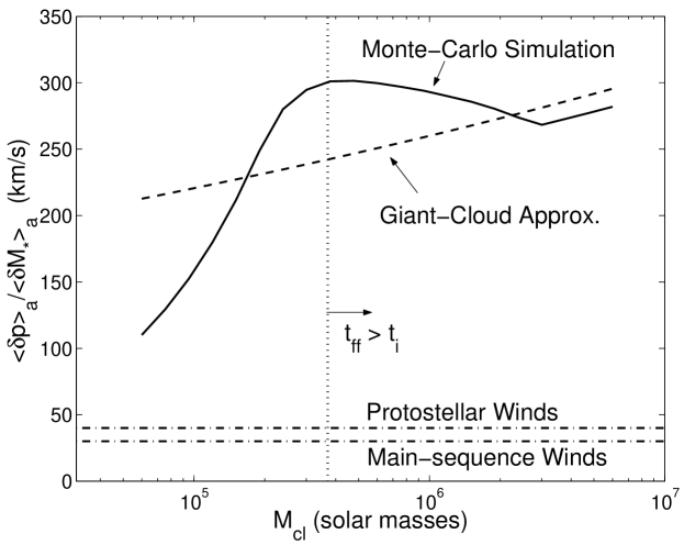
Figure 1.— Cloud momentum generated by H II regions per stellar mass formed, and an illustration of the giant-cloud approximation. The theory for H II regions presented here does not account for gravity and is therefore only valid for clouds to the right of the vertical dotted line – those whose free-fall times are longer than the ionizing lifetimes of OB associations (eq. [23]). The solid line is the result of Monte-Carlo simulations that account for the difference between the Galactic H II region luminosity function and what is expected within a given cloud (eq. [35]; see also MW97). These simulations also account for the effect of finite cloud size. The dashed line represents the giant-cloud approximation in which both the corrections to the Galactic luminosity function and the finite-size effects are ignored. To the right of the dotted line, differences between the two curves result primarily from the luminosity function (and are relatively minor): for instance, the kink at $M_{\rm cl}=3\times 10^{6}~{}M_{\odot}$ divides clouds that can harbor the largest Galactic OB associations from those that cannot. Finite cloud-size effects dominate to the left of the dotted line, where our model of H II regions is already invalidated by gravity. The dash-dot lines show the momenta of protostellar and main-sequence winds in the first 3.7 Myr of a cluster’s life.

For clouds with $M_{\rm cl,6}<3.7$ it might be more appropriate to take a small-cloud approximation in which all H II regions are assumed to outgrow their clouds: $\delta M_{\rm dest}=\delta M_{\rm dest,max}$, $\delta p=\delta p_{\rm max}$, and $r_{m}=R_{\rm cl}$ (cf. MW97 eq. [41]). This would be very uncertain, however, both because our estimates of $\delta M_{\rm dest,max}$ and $\delta p_{\rm max}$ are uncertain and also because we have neglected cloud gravity, which should be important when $M_{\rm cl}<3.7\times 10^{5}~{}M_{\odot}$.

The performance of the giant-cloud approximation is illustrated in figure 1, where we plot its prediction for $\left<\delta p\right>_{a}$ (dashed line, eq. [18]) against the results of a Monte-Carlo simulation (solid line). The simulation accounts for the difference between the luminosity distribution of OB associations within a given GMC ($F_{a,M}$, eq. [35]) and that within the Galaxy as a whole ($F_{a}$, eq. [32]), whereas this distinction is neglected in the giant-cloud approximation. This is the primary cause for the difference between the two curves for $M_{\rm cl}>3.7\times 10^{5}~{}M_{\odot}$, to the right of the vertical dotted line; for instance, the kink in the simulation at $M_{\rm cl,6}=3$ is caused by the kink in $F_{a,M}$ in equation (35). The simulation also accounts for finite-size effects ($\delta p_{\rm max}$, eq. [21]); these dominate the difference between the curves to the left of the dotted line. However, our neglect of cloud gravity is not valid in that region (eq. [23]).

4.2. Momentum Generation

A comparison between $\left<\delta p\right>_{a}$ and $\left<M_{\star}\right>_{a}$ gives the effective input of momentum per stellar mass averaged over H II regions. In the giant-cloud approximation, an integral of equation (18) over $F_{a}(>S_{49})$ gives

$$\left<\delta p\right>_{a}\simeq 260\left(\frac{N_{H,22}}{1.5}\right)^{-3/14}M_{\rm cl,6}^{1/14}~{}{\rm km~{}s^{-1}}\times\left<M_{\star}\right>_{a}.$$ (36)

The characteristic velocity (momentum per stellar mass) identified in this equation is much larger than the corresponding coefficient $\delta p_{w}/m_{\star}=40\phi_{w}{\rm km~{}s^{-1}}$ that we have estimated for protostellar winds in equation (5), or the value $38~{}{\rm km~{}s^{-1}}$ estimated for main-sequence and evolved star ejecta in equation (24). Since equation (36) applies to both blister-type and embedded H II regions, it implies that H II regions are more important than the combined effects of protostellar winds, stellar winds, and supernovae in driving turbulence within GMCs, regardless of the efficiency of star formation. Figure 1 makes this point graphically.

Our estimate of $\delta p_{\rm dest,max}$ indicates that H II regions dominate over protostellar winds so long as $M_{\rm cl}\gtrsim 4\times 10^{4}~{}M_{\odot}$. This, in turn, suggests that protostellar winds may support small clouds and the self-gravitating clumps within GMCs (Bertoldi & McKee 1996; Matzner & McKee 1999b), whereas H II regions support the GMCs themselves.

4.3. Mass Ejection

If we assume that all H II regions evolve into blister regions, as have Whitworth (1979), Franco et al. (1994), and WM97, we arrive at an upper limit to the amount of mass than can be removed from a GMC by photoevaporation. Since $\delta p=2c_{\rm II}\delta M_{\rm dest}$ for a blister region, equation (36) gives, in the giant-cloud approximation,

$$\left<\delta M_{\rm dest}\right>_{a}\simeq 14\left(\frac{N_{H,22}}{1.5}\right)^{-3/14}M_{\rm cl,6}^{1/14}\times\left<M_{\star}\right>_{a},$$ (37)

implying a typical instantaneous star formation efficiency

$$\varepsilon\equiv\frac{\left<M_{\star}\right>_{a}}{\left<\delta M_{\rm dest}\right>_{a}+\left<M_{\star}\right>_{a}}\simeq 6.7\%\times\left(\frac{N_{H,22}}{1.5}\right)^{3/14}M_{\rm cl,6}^{-1/14}$$ (38)

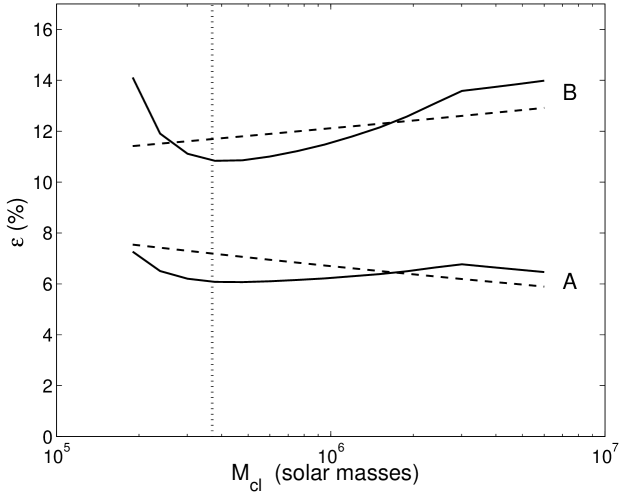
Figure 2.— Star formation efficiency in giant clouds, assuming photoevaporation is the dominant disruption mechanism. The curves marked A are not corrected for the interaction between H II regions, whereas the curves marked B account self-consistently for finite cloud porosity (§7). The solid lines are Monte-Carlo calculations based on MW97’s model for the luminosity functions of OB associations forming within a given cloud; effects due to finite cloud size (eqs. [20], [21], and [28]) are included. The dashed lines are analytical results of the giant-cloud approximation (§4.1): equations (38) and (51) for cases A and B, respectively. In this and subsequent figures we assume that all H II regions enter the blister stage (see §7).

${\rm SFE_{\rm tot}}$ and $\varepsilon$ are related by ${\rm SFE_{\rm tot}}=\left<\varepsilon^{-1}\right>^{-1}$ (Matzner & McKee 2000); however, a sudden disruption of the cloud (a precipitous drop of $\varepsilon$, as discussed in §3.3) would reduce ${\rm SFE_{\rm tot}}$ below the typical value of $\varepsilon$.

The lines marked A in figure 2 compare equation (38) with the results of a Monte-Carlo simulation which accounts for the birthrates of OB associations within individual clouds as given by equation (35). The lines marked B account self-consistently for the frequent interaction between H II regions, in a manner we discuss in §7.

Unfortunately, there are insufficient observations of clouds in the mass range $3.7\times 10^{5}~{}M_{\odot}<M_{\rm cl}<6\times 10^{6}~{}M_{\odot}$ to test equation (38) directly. Observations of nearby clouds, which are too small for an application of our theory, indicate a significantly lower star formation efficiency than an extrapolation of our theory would predict: for instance, observations of nearby small clouds (Evans & Lada 1991) indicate that only $\sim 1\%$ of the mass is stellar and only $\sim 3\%$ will ever be. Besides gravity, a number of other effects may be important for clouds this small; WM97 have emphasized their disruption by H II regions that outgrow their boundaries (see also Elmegreen 1979), as well as the likelihood that this disruption will render them susceptible to photodissociation.

5. Ionizing Luminosity and Star Formation Rate

As a cloud’s turbulence decays it must be replenished, if virial balance is to be maintained. Energy can be derived from gravitational contraction, winds and supernovae, and H II regions. Contraction is problematic as it would imply a collapse rate close to free-fall, hence rapid star formation; this may hold for the formation of stellar associations, but cannot for entire GMCs (Zuckerman & Palmer 1974).

We have shown that H II regions are the most effective of the remaining sources. Accordingly we will match the loss of turbulent momentum with its regeneration in H II regions. We must account for a population of H II regions with different luminosities and therefore different values of $\delta p$, $r_{m}$, and $\lambda_{\rm in}$. Equations (1) and (3) predict that energy decays in a time proportional to $\lambda_{\rm in}$. It is most consistent to assume that the contribution from each type of H II region decays independently on its own timescale; the total turbulent energy is then the sum of these decaying contributions. Taking the decay time from equation (3), and taking the energy input $\delta E_{\rm turb}(\delta p)$ from equation (4),

$$E_{\rm turb} = \sum_{S_{49}}\delta E_{\rm turb}\times({\rm decay~{}time})\times({\rm rate})$$ (39)

$$= \frac{\phi c_{\rm eff}\dot{\cal N}_{a}}{2.4v_{\rm rms}}\left<\lambda_{\rm in}(\delta p)\delta p\right>_{a},$$

where $\lambda_{\rm in}(\delta p)$ is given by equations (28) and (30) and $\dot{\cal N}_{a}$ is the formation rate of associations.

Applied to a GMC, equation (39) must be consistent with the observed kinetic energy of the cloud and the expected degree of equipartition between kinetic and magnetic energy (eq. [2]). Equating expressions (2) and (39) gives the formation rate of associations:

$$\dot{\cal N}_{a}=\frac{1.9M_{\rm cl}v_{\rm rms}^{3}}{\phi c_{\rm eff}\left<\lambda_{\rm in}(\delta p)\delta p\right>_{a}}.$$ (40)

If one were to vary the ionizing flux of all stars in the IMF by the same factor, then $\dot{\cal N}_{a}$ would vary as $1/(\lambda_{\rm in}\delta p)\propto(\delta p)^{-4/3}\propto\left<S_{49}\right>_{a}^{-16/21}\propto\left<s_{49}\right>^{-16/21}$. This scaling holds also for the star formation rate $\dot{M}_{\star}=\left<M_{\star}\right>_{a}\dot{\cal N}_{a}$. But, the mean ionizing flux produced by these associations would vary much less: $S_{49,T}(M_{\rm cl})\equiv\left<S_{49}\right>_{a}\left<t\right>_{\rm ms}\dot{\cal N}_{a}\propto\left<s_{49}\right>^{5/21}$. This is not surprising, as the ionizing photons are directly responsible for sustaining equilibrium.

A cloud’s ionizing luminosity is therefore quantity most tightly constrained by the assumption of equilibrium: in the giant-cloud approximation,

$$S_{49,T}(M_{\rm cl}) = \frac{(37,53)}{\phi_{m}(\phi/1.6)}\left(\frac{N_{H,22}}{1.5}\right)^{1.37}\left(\frac{c_{\rm eff}}{0.57v_{\rm rms}}\right)^{-2/3}$$ (41)

$$\times M_{\rm cl,6}^{37/28}.$$

for H II regions that are primarily in the (embedded, blister) state, respectively. This equation will be adjusted for the interaction between H II regions in §7. To compare with observations of individual clouds one must account for the leakage of ionizing photons; MW97 estimate that $\sim 70\%$ escape the observed H II regions.

The star formation rate is $\dot{M}_{\star}=\left<M_{\star}\right>_{a}\dot{\cal N}_{a}$. Using the giant-cloud approximation and MW97’s IMF,

$$\dot{M}_{\star} \simeq \frac{(5.7,8.2)\times 10^{-3}}{\phi_{m}(\phi/1.6)}\left(\frac{N_{H,22}}{1.5}\right)^{1.37}\left(\frac{c_{\rm eff}}{0.57v_{\rm rms}}\right)^{-2/3}$$ (42)

$$\times M_{\rm cl,6}^{37/28}~{}M_{\odot}~{}{\rm yr}^{-1}$$

for (embedded, blister) regions. Recall that $\dot{M}_{\star}\propto\left<m_{\star}\right>\left<s_{49}\right>^{-16/21}$ is predicted less robustly than $S_{49,T}(M_{\rm cl})\propto\left<s_{49}\right>^{5/21}$ due to uncertainties in the mean stellar mass and ionizing luminosity. Kennicutt et al. (1994) find that the ratio $\left<m_{\star}\right>/(\left<s_{49}\right>\left<t_{\rm ms}\right>)$ varies by about $50\%$ among the forms of the IMF and sets of stellar tracks they consider; the predicted $\dot{M}_{\star}$ is therefore uncertain by at least this amount.

The mean ionizing luminosity and lifetime depend on the metallicity $Z$ of the stellar population, and these effects cause a shift in the star formation rate relative to equation (42) even if the IMF remains constant. Numerical integrations of equation (15), performed for Starburst99 populations of various $Z$, exhibit $\left<\delta p\right>_{a}/\left<M_{\star}\right>_{a}\propto Z^{-0.092}$ implying $\dot{M}_{\star}\propto Z^{0.12}N_{H}^{1.37}$. In any situation where M89’s theory holds, $N_{H}\propto Z^{-1}$ and therefore $\dot{M}_{\star}\propto Z^{-1.25}$.

Figure 3.— The time scale for molecular gas to be converted into stars, $t_{g*}\equiv M_{\rm cl}/\dot{M}_{\star}$. Here, as in the other figures, the vertical dotted line delimits the lower mass limit of validity of our theory (eq. [23]); the solid lines are Monte-Carlo calculations. The dashed lines are the giant-cloud approximation, equations (42) and (49) for A and B, respectively. The curves marked A neglect interactions between H II regions, whereas those marked B account self-consistently for these interactions in the manner derived in §7. The value of $t_{g*}$ for the entire Galaxy is plotted as the dash-dot line; this corresponds to a total molecular mass of $10^{9}~{}M_{\odot}$ and star formation rate of $5.1~{}M_{\odot}$ per year (Mezger 1987). Also plotted is the value of $t_{g*}$ implied by Carpenter (2000)’s determination that the nearby Perseus, Orion A, Orion B, and Mon R2 clouds ($10^{4}~{}M_{\odot}<M_{\rm cl}<3\times 10^{4}~{}M_{\odot}$) have converted $\sim 1.6\%$ of their mass into stars in the past 3-7 Myr. In this figure the product $\phi_{m}\phi$ is taken to be $1.6\times 1.2$.

Our hypothesis that the star formation rate is determined by a balance between the dissipation of turbulence and its regeneration in H II regions can only make sense if it predicts more than one H II region per dynamical time of the cloud. This is true for all the clouds within the regime of validity of our theory, as we find that $\dot{\cal N}_{a}t_{\rm ff}\gtrsim(13,19)\times N_{H,22}^{13/21}(1.6/[\phi_{m}\phi])$ so long as $M_{\rm cl,6}>0.37$.

In figure 3 we plot $t_{g*}\equiv M_{\rm cl}/\dot{M}_{\star}$, the time scale for gas to be converted into stars. Equation (42) is shown as the dashed curve marked A. The solid curve marked A is the results of a Monte-Carlo simulation which incorporates equation (32) and the effects of finite cloud size (eqs. [21] and [28]). The curves marked B are adjusted to account for the interaction between H II regions, as described in §7. Also plotted (dash-dot line) is value of $t_{g*}$ appropriate to the entire inner Galaxy, and the range suggested by Carpenter (2000)’s observations of clouds around $2\times 10^{4}~{}M_{\odot}$, 190-440 Myr (corresponding to the acceptable age range 3-7 Myr for the embedded population; see below).

5.1. Galactic Ionizing Luminosity and Star Formation Rate

Equations (41) and (42) refer only to a single molecular cloud. Integrating over the GMC population for the inner Galaxy, we arrive at the total inner-Galactic ionizing luminosity $S_{T}$ and star formation rate $\dot{M}_{\star T}$. WM97 model the GMC population of the inner galaxy as $dN_{\rm cl}/d\ln M_{\rm cl}\simeq 63(6/M_{\rm cl,6})^{-0.6}$; setting $N_{H,22}=1.5$ as observed, and considering only giant clouds with $M_{\rm cl,6}>3.7$ for which we are relatively confident of the star formation rate, we find

$$S_{T}\simeq\frac{(3.0,4.3)\times 10^{53}}{\phi_{m}(\phi/1.6)}\left(\frac{c_{\rm eff}}{0.57v_{\rm rms}}\right)^{-2/3}~{}{\rm s}^{-1}$$ (43)

and

$$\dot{M}_{\star T}\simeq\frac{(4.6,6.6)}{\phi_{m}(\phi/1.6)}\left(\frac{c_{\rm eff}}{0.57v_{\rm rms}}\right)^{-2/3}~{}M_{\odot}~{}{\rm yr}^{-1}.$$ (44)

These results would be $15\%$ higher if we were to extrapolate the giant-cloud approximation below the lower limit of $M_{\rm cl,6}=0.37$. As before, $S_{T}$ is much better constrained than $\dot{M}_{\star T}$ by our hypothesis that H II regions dominate feedback.

We may use observations to check that clouds with $M_{\rm cl,6}<0.37$, whose evolution we cannot address, do not dominate the Galactic star formation rate or ionizing flux. Consider Carpenter (2000)’s observations of the Perseus, Orion A, Orion B, and Mon R2 clouds ($M_{\rm cl}\sim 1-3\times 10^{4}~{}M_{\odot}$ for each). Carpenter estimated the completeness of the 2MASS survey and the resulting stellar fraction in these clouds, a slowly increasing function of the assumed age of the observed stellar population. Carpenter argues that that these clouds have created a stellar mass equal to $\sim 1.6\%$ of their own mass in a period between 3 and 7 Myr. Extrapolating this star formation rate per unit molecular mass to all clouds with $M_{\rm cl,6}<0.37$, using MW97’s cloud mass function, gives a range of 0.7 to 1.7 $M_{\odot}$ per year. This estimate should be considered very uncertain, as it assumes $\dot{M}_{\star}\propto M_{\rm cl}$ for small clouds; however it indicates that clouds in the mass range $M_{\rm cl}<3.7\times 10^{5}~{}M_{\odot}$, which constitute one third of the molecular mass, most likely do not dominate the Galactic star formation rate.

MW97 estimate the ionizing flux of the inner Galaxy at $2.6\times 10^{53}~{}{\rm s}^{-1}$ (assuming all ionizing photons are caught within the disk) and derive a star formation rate of $4.0~{}M_{\odot}~{}{\rm yr}^{-1}$. [Mezger (1987) estimates the star formation rate in the inner Galaxy to be $5.1~{}M_{\odot}~{}{\rm yr}^{-1}$.] Equations (43) and (44) are comparable to this value, with $\phi\simeq 1.6$ as suggested by McKee (1999), and with $\phi_{m}\simeq 1.1$ (close to unity as suggested in §3.4). Given the approximations that led to equation (44), this degree of agreement is quite remarkable; it supports our proposition that feedback from H II regions regulates the rate of star formation in giant molecular clouds.

6. Lifetimes of GMCs

We may combine the star formation rate given in equation (42) with the upper limit for mass evaporation from GMCs given in equation (37), to arrive at a lower limit for the lifetime of GMCs assuming all H II regions evolve into blister regions. In the giant-cloud approximation, this gives

$$t_{d0}\equiv\frac{M_{\rm cl}}{\dot{M}_{\rm dest}} \simeq 13\phi_{m}\left(\frac{\phi}{1.6}\right)\left(\frac{N_{H,22}}{1.5}\right)^{-1.15}$$ (45)

$$\times\left(\frac{c_{\rm eff}}{0.57v_{\rm rms}}\right)^{2/3}M_{\rm cl,6}^{-11/28}~{}{\rm Myr}.$$

for $M_{\rm cl}>3.7\times 10^{5}~{}M_{\odot}$. A significant population of H II regions that remain embedded rather than evolving into blister regions would extend this lifetime, but we argue in §7 that such a population is not likely. Another effect that extends cloud lifetimes relative to $t_{d0}$ is the finite porosity of H II regions within their volumes (MW97), for which we account in §7.

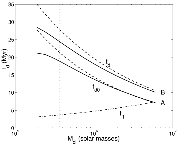
Figure 4.— Destruction time scales $t_{d0}$ (case A, ignoring cloud porosity) and $t_{d}$ (case B, accounting for finite porosity) for giant clouds. The solid lines are Monte-Carlo calculations; the dash-dot lines, which result from the giant-cloud approximation, represent equations (45) and (50) for cases A and B, respectively. Also plotted is the clouds’ free-fall time $t_{\rm ff}$, which approaches their destruction time at the upper mass limit for Galactic GMCs.

Note that the estimate of the cloud destruction time in equation (45) is roughly $2.6M_{\rm cl,6}^{-4/7}$ times longer than the cloud’s free-fall time; the two time scales are equal for a mass $M_{\rm cl}=5.3\times 10^{6}(N_{H,22}/1.5)^{-13/12}~{}M_{\odot}$, very close to the upper mass limit for Galactic GMCs ($\sim 6\times 10^{6}~{}M_{\odot}$; WM97). This raises the possibility that the upper mass limit derives from the difficulty of assembling an object that destroys itself rapidly compared to its free-fall time scale, a hypothesis that should be tested against extragalactic observations. We refine this argument in §7, where we adjust the destruction time for finite cloud porosity. (But note, a possible counterargument is raised in §8.)

Cloud destruction timescales are plotted in figure 4, where our Monte-Carlo simulation (solid lines) is compared with the results of the giant-cloud approximation as given by equations (45) and (50) for cases A and B, respectively. The curves marked B are adjusted for the interaction between H II regions (§7). The free-fall time is also plotted, making visible the crisis of rapid destruction for clouds above the Galactic upper mass limit.

Our equation (45) is based on the same physics that led MW97 to estimate a destruction time of 20-25 Myr for clouds with $M_{\rm cl,6}>0.1$. Our estimate is shorter because MW97 assumed $\dot{M}_{\star}\propto M_{\rm cl}$, whereas an energetic balance requires $\dot{M}_{\star}\propto M_{\rm cl}^{1.3}$ in our giant-cloud approximation; this redistribution shortens the lives of the massive clouds to which our theory applies.

7. Effect of Finite Porosity

The frequency with which H II regions form within GMCs implies that they are likely to interact (WM97). Defining the porosity $Q$ as the time-averaged volume filling factor of H II regions, $Q\equiv\dot{\cal N}_{a}\int\int^{t_{\rm ms}}[M_{\rm sh}(t)/M_{\rm cl}]dt\,dF_{a}$, we estimate from the above equations

$$Q_{0} = \frac{(2.6,4.2)}{{\phi_{m}}(\phi/{1.6})}\times\left(\frac{N_{H,22}}{1.5}\right)^{19/12}$$ (46)

$$\times\left(\frac{c_{\rm eff}}{0.57v_{\rm rms}}\right)^{-2/3}M_{\rm cl,6}^{1/4}$$

for (blister, embedded) regions respectively. This expression is not yet fully self-consistent; we find $Q$ in terms of $Q_{0}$ below. The large value of $Q_{0}$ for embedded regions implies that fully embedded H II regions are ruled out, as H II regions will percolate and allow their gas to vent. This reinforces our neglect of embedded regions in equation (45).

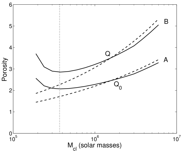
Figure 5.— The porosity of H II regions within GMCs. Plotted are the initial estimate ($Q_{0}$, case A), which does not account self-consistently for the effect of porosity on star formation rate, and the revised estimate ($Q$, case B), which does. The dashed lines result from the giant-cloud approximation; case A is given by equation (46).

WM97 argue that the effect of interactions is equivalent to regrouping stars into non-interacting regions that are larger by the factor $(1+Q)$, i.e., $\dot{\cal N}_{a}^{\prime}=\dot{\cal N}_{a}/(1+Q)$ and $S_{49}^{\prime}=(1+Q)S_{49}$. For each of the regrouped regions, $\delta p^{\prime}=(1+Q)^{4/7}\delta p$, $\delta M_{\rm dest}^{\prime}=(1+Q)^{4/7}\delta M_{\rm dest}$, and, for the giant-cloud approximation ($r_{m}<R_{\rm cl}$), $\lambda_{\rm in}^{\prime}=(1+Q)^{4/21}\lambda_{\rm in}$. Whereas WM97 assumed a star formation rate within a given cloud, our theory demands that we determine the star formation rate self-consistently by matching turbulent decay with driving by H II regions. Applying these transformations to equation (40) and eliminating $\dot{\cal N}_{a}^{\prime}$, we find that $\dot{\cal N}_{a}=(1+Q)^{5/21}\dot{\cal N}_{a0}$ where $\dot{\cal N}_{a0}$ is the uncorrected value in equation (40). But, the porosity is proportional the star formation rate: $Q=Q_{0}\dot{\cal N}_{a}/\dot{\cal N}_{a0}$. A self-consistent value of $Q$ therefore satisfies

$${Q}{(1+Q)^{-5/21}}=Q_{0},$$ (47)

so that $Q\simeq Q_{0}$ when $Q_{0}<1$, but $Q\simeq Q_{0}^{21/16}$ when $Q_{0}\gg 1$. We find that the useful relation $(1+Q)=1.85Q_{0}$ holds within $1\%$ in the cloud mass range of interest. The analytical (equation [46]) and numerical values of $Q_{0}$ and $Q$ are plotted in figure 5.

To account self-consistently for finite porosity, we must increase $\dot{\cal N}_{a}$, $S_{49,T}(M_{\rm cl})$ and $\dot{M}_{\star}$ by $(1+Q)^{5/21}$ relative to equations (40), (41), and (42), increase the cloud lifetimes by $(1+Q)^{4/21}$ relative to equation (45), and increase the stellar mass per ejected mass $(\varepsilon^{-1}-1)^{-1}\simeq\varepsilon$ by $(1+Q)^{3/7}$ relative to equation (38). The revised equations are

$$S_{49}(M_{\rm cl}) \simeq \frac{54}{\left[\phi_{m}(\phi/1.6)\right]^{26/21}}\left(\frac{N_{H,22}}{1.5}\right)^{1.75}\left(\frac{c_{\rm eff}}{0.57v_{\rm rms}}\right)^{-0.83}$$ (48)

$$\times M_{\rm cl,6}^{1.38}~{}M_{\odot}~{}{\rm yr}^{-1},$$

$$\dot{M}_{\star} \simeq \frac{8.3\times 10^{-3}}{\left[\phi_{m}(\phi/1.6)\right]^{26/21}}\left(\frac{N_{H,22}}{1.5}\right)^{1.75}\left(\frac{c_{\rm eff}}{0.57v_{\rm rms}}\right)^{-0.83}$$ (49)

$$\times M_{\rm cl,6}^{1.38}~{}M_{\odot}~{}{\rm yr}^{-1},$$

$$t_{d} \simeq 17\left[\phi_{m}\left(\frac{\phi}{1.6}\right)\right]^{0.81}\left(\frac{N_{H,22}}{1.5}\right)^{-0.85}$$ (50)

$$\times\left(\frac{c_{\rm eff}}{0.57v_{\rm rms}}\right)^{0.54}M_{\rm cl,6}^{-0.35}~{}{\rm Myr},$$

and

$$\varepsilon \simeq {13}\%\times{\left[\phi_{m}\left(\frac{\phi}{1.6}\right)\right]^{-3/7}}\left(\frac{N_{H,22}}{1.5}\right)^{0.89}$$ (51)

$$\times\left(\frac{c_{\rm eff}}{0.57v_{\rm rms}}\right)^{-2/7}M_{\rm cl,6}^{1/28},$$

respectively. The corrected lifetime is $1.2(\phi_{m}\phi/1.6)^{0.81}(M_{\rm cl,6}/6)^{-0.6}t_{\rm ff}$, i.e., just over one free-fall time at the upper mass limit for Galactic GMCs. The total ionizing luminosity and star formation rate in the inner Galaxy due to clouds in the mass range $3.7\times 10^{5}~{}M_{\odot}<M_{\rm cl}<6\times 10^{6}~{}M_{\odot}$ become $4.5\times 10^{53}(\phi_{m}\phi/1.6)^{-26/21}~{}{\rm s}^{-1}$ and $7.0(\phi_{m}\phi/1.6)^{-26/21}~{}M_{\odot}~{}{\rm yr}^{-1}$, respectively. These are consistent with the observed rate if $\phi\simeq 1.6$ and $\phi_{m}\simeq 1.6$.

Thus, our estimates of the Galaxy’s ionizing luminosity and star formation rate (with $\phi_{m}\phi\simeq 1\times 1.6$) are comparable to the values adopted by MW97 if cloud porosity is not accounted for (consistency requiring $\phi_{m}\phi\simeq 1.1\times 1.6$) and somewhat higher (consistency requiring $\phi_{m}\phi\simeq 1.6\times 1.6$) after the porosity correction is applied. This level of agreement suggests H II regions are indeed responsible for maintaining energetic equilibrium within GMCs. What might explain the remaining discrepancy? First, numerical estimates of turbulent decay rates may decrease as studies improve in resolution and less diffusive codes are used, or as turbulent anisotropy is included (Cho et al. 2001). Second, the Galaxy’s ionizing luminosity could be higher than MW97 found, if a significant fraction of ionizing photons escape the Galactic disk (unlikely, but controversial; Bland-Hawthorn & Putman 2001) – but conversely, additional ionization from sources like supernova remnants (Slavin et al. 2000) would increase the discrepancy. Third, the discrepancy results from our method of accounting for finite porosity, a crude approximation when $Q>1$. Fourth, we were not entirely able to exclude a contribution of momentum from supernovae in §3.2, especially for small associations.

Lastly, we have followed MW97 in approximating clusters’ ionizing luminosity as a step function of duration $\left<t_{\rm ms}\right>=3.7$ Myr. In reality, a numerical integration of equation (15) using the ionization history predicted by a Starburst99 synthesis indicates that $\delta p$ continues to grow (albeit more slowly), gaining another $50\%$ after 6.6 Myr. This should effectively increase $\left<t_{\rm ms}\right>$ in the largest clouds, whose free-fall times are long enough to permit this expansion. All of these topics merit further study.

8. Conclusions

The main results of this paper are as follows.

1. H II regions are the most plentiful sources of energy for the turbulence within giant molecular clouds; they are more significant than the combined effects of protostellar winds, main-sequence and evolved-star winds, and supernovae. This result was indicated by the low efficiency of star formation in GMCs in §2.1 and demonstrated on more general grounds in §§3.2 and 4.2.

2. The input of turbulent energy by H II regions occurs on scales comparable to, but somewhat smaller than, the cloud radius. Large-scale forcing minimizes the rate of turbulent decay, as recently emphasized by Basu & Murali (2001).

3. A balance between turbulent decay and the regeneration of turbulence by H II regions allows a prediction of the stellar ionizing luminosity and (less robustly) the star formation rate. We present these results for clouds in the mass range $3.7\times 10^{5}~{}M_{\odot}<M_{\rm cl}<6\times 10^{6}~{}M_{\odot}$, in which the stellar ionizing lifetime is briefer than the free-fall time. The results are roughly consistent with the total ionizing luminosity and star formation rate of the inner Galaxy, provided that future numerical simulations verify our estimate of the coupling between momentum input and turbulent energy (eq. [31]). Our estimate of the ionizing flux in the inner Galaxy is $\sim 70\%$ higher than the observed value; we list in §7 several possible resolutions of this discrepancy.

4. Because H II regions also evaporate their clouds, an energetic balance also implies a rate of photoevaporation and a destruction time scale for GMCs. We derive a destruction time of 17 to 24 times $(M_{\rm cl}/10^{6}M_{\odot})^{-1/3}$ million years, somewhat shorter than was found by WM97.

5. The upper mass limit for Milky Way GMCs most likely derives from the difficulty of assembling an object that destroys itself in a single crossing time. However, less massive clouds (at least down to $3.7\times 10^{5}~{}M_{\odot}$) survive for many crossing times, produce many H II regions per crossing time, and are in both energetic and dynamical equilibrium.

6. So long as there exists a minimum optical depth or column density required for star formation, the vigorous energetic feedback by H II regions provides a mechanism for the maintenance of cloud column densities near the critical value, and hence, for the GMC line width-size relation. Massive clouds therefore follow the scenario proposed by M89, but with H II regions rather than protostellar winds as the primary agents of feedback. This conclusion is not assured for clouds less massive than $3.7\times 10^{5}~{}M_{\odot}$, for which cloud gravity must be considered in the dynamics of H II regions.

The theory we have presented is robust, in the sense that it applies to massive GMCs (containing the bulk of the molecular mass) and derives from the flattening of the luminosity function between rich and poor OB associations – a product solely of the upper mass limit for stars – rather than the detailed birthrate distribution of OB associations. So long as a galaxy’s molecular mass is concentrated in the most massive clouds, and so long as the birthrate of stellar associations drops with ionizing luminosity more steeply than $d\dot{\cal N}_{a}/d\ln S_{49}\propto S_{49}^{-4/7}$, energetic equilibrium within molecular clouds determines its ionizing flux. This assertion can be tested by extragalactic observations. Starbursts may however be an exception to this rule if, as discussed below, their GMCs are not in equilibrium.

Other observational tests of the theory presented here include the variation of ionizing luminosity and star formation rate (figure 3) with cloud mass and the high porosity of HII regions (figure 5) for massive GMCs. The variations of these quantities with mean cloud column density can potentially be tested by observations of the SMC. The star formation efficiency (figure 2) and cloud lifetime (figure 4) will be more difficult to verify.

The inhomogeneity of giant molecular clouds is the greatest source of uncertainty in the present work. The interaction of H II regions – one source of inhomogeneity – was treated in an approximate manner in §7, but future work must treat the interaction of H II regions with a realistic background cloud.

We have noted that clouds more massive than $6\times 10^{6}~{}M_{\odot}$ should not form in the Milky Way because they would be disrupted by H II regions in the time needed to assemble them. However, we must also note that clouds more massive than about $3.7\times 10^{6}(N_{H,22}/1.5)^{-1}~{}M_{\odot}$ may be incapable of driving champagne flows because their escape velocities exceed the exhaust velocity $\phi_{\rm II}c_{\rm II}=19.4~{}{\rm km~{}s^{-1}}$ of ionized gas. This fact does not affect our derivation of the star formation rate in such clouds, but it does call into question our derivation of the lifetime for the most massive clouds (and hence our suggestion for the origin of the upper mass limit). Further work will be needed to resolve this issue.

Similarly, clouds more massive than about $1.9\times 10^{7}(N_{H,22}/1.5)^{-1}~{}M_{\odot}$ cannot have supersonic H II regions, as their effective sound speeds exceed $10~{}{\rm km~{}s^{-1}}$, the sound speed of ionized gas. Objects created in this state or pushed into it by an increase in external pressure can neither be disrupted nor even supported by photoionization, and must collapse as rapidly as their turbulence decays; this is a recipe for the efficient production of massive star clusters observed to occur in starburst galaxies. For instance, Scoville et al. (1991) find values of $N_{H,22}$ in the range $10^{3}$ to $10^{4.5}$ for the mean central molecular gas in a number of starbursts; this is sufficient to crush all GMCs in the mass range $M_{\rm cl}>3.7\times 10^{5}~{}M_{\odot}$.

References

- Arons & Max (1975) Arons, J. & Max, C. E. 1975, ApJ, 196, L77
- Ballesteros-Paredes et al. (1999a) Ballesteros-Paredes, J., Hartmann, L., & Vázquez-Semadeni, E. 1999a, ApJ, 527, 285
- Ballesteros-Paredes et al. (1999b) Ballesteros-Paredes, J., Vázquez-Semadeni, E., & Scalo, J. 1999b, ApJ, 515, 286
- Basu & Murali (2001) Basu, S. & Murali, C. 2001, ApJ, 551, 743
- Bertoldi & McKee (1990) Bertoldi, F. & McKee, C. F. 1990, ApJ, 354, 529
- Bertoldi & McKee (1992) —. 1992, ApJ, 395, 140
- Bertoldi & McKee (1996) Bertoldi, F. & McKee, C. F. 1996, in Amazing Light: A Volume Dedicated to C.H. Townes on his 80th Birthday, ed. R.Y.Chiao (New York: Springer), 41
- Bland-Hawthorn & Putman (2001) Bland-Hawthorn, J. & Putman, M. E. 2001, in Gas and Galaxy Evolution, ASP Conf. 240, eds. J.E. Hibbard, M.P. Rupen, J.H. van Gorkom, 369
- Blitz & Shu (1980) Blitz, L. & Shu, F. H. 1980, ApJ, 238, 148
- Carpenter (2000) Carpenter, J. M. 2000, AJ, 120, 3139
- Chevalier (1999) Chevalier, R. A. 1999, ApJ, 511, 798
- Cho et al. (2001) Cho, J., Lazarian, A., & Vishniac, E. 2001, accepted by ApJ
- Cioffi et al. (1988) Cioffi, D. F., McKee, C. F., & Bertschinger, E. 1988, ApJ, 334, 252
- Cohen & Kuhi (1979) Cohen, M. & Kuhi, L. V. 1979, ApJS, 41, 743
- Dyson et al. (1995) Dyson, J. E., Williams, R. J. R., & Redman, M. P. 1995, MNRAS, 277, 700
- Elmegreen (1979) Elmegreen, B. G. 1979, ApJ, 231, 372
- Elmegreen (1983) —. 1983, MNRAS, 203, 1011
- Elmegreen (2000) —. 2000, ApJ, 530, 277
- Evans & Lada (1991) Evans, N. J. & Lada, E. A. 1991, in IAU Symp. 147: Fragmentation of Molecular Clouds and Star Formation, Vol. 147, 293
- Franco & Cox (1983) Franco, J. & Cox, D. P. 1983, ApJ, 273, 243
- Franco et al. (1994) Franco, J., Shore, S. N., & Tenorio-Tagle, G. 1994, ApJ, 436, 795
- García-Segura & Franco (1996) García-Segura, G. & Franco, J. 1996, ApJ, 469, 171
- Hartmann et al. (2001) Hartmann, L., Ballesteros-Paredes, J., & Bergin, E. A. 2001, accepted by ApJ
- Jijina & Adams (1996) Jijina, J. & Adams, F. C. 1996, ApJ, 462, 874
- Kahn (1954) Kahn, F. D. 1954, Bull. Astron. Inst. Netherlands, 12, 187
- Kennicutt et al. (1989) Kennicutt, R. C., Edgar, B. K., & Hodge, P. W. 1989, ApJ, 337, 761
- Kennicutt et al. (1994) Kennicutt, R. C., Tamblyn, P., & Congdon, C. E. 1994, ApJ, 435, 22
- Koo & McKee (1992) Koo, B.-C. & McKee, C. F. 1992, ApJ, 388, 93
- Lada & Gautier (1982) Lada, C. J. & Gautier, T. N. 1982, ApJ, 261, 161
- Larson (1981) Larson, R. B. 1981, MNRAS, 194, 809
- Leitherer et al. (1999) Leitherer, C., Schaerer, D., Goldader, J. D., Delgado, R. M. G., Robert, C., Kune, D. F., de Mello, D. F., Devost, D., & Heckman, T. M. 1999, ApJS, 123, 3
- Mac Low (1999) Mac Low, M.-M. 1999, ApJ, 524, 169
- Mac Low (2000) Mac Low, M.-M. 2000, in Star formation from the small to the large scale. ESLAB symposium 33 Noordwijk, The Netherlands. Edited by F. Favata, A. Kaas, and A. Wilson., 457
- Mac Low et al. (2001) Mac Low, M.-M., Balsara, D., Avillez, M. A., & Kim, J. 2001, submitted to ApJ
- Mac Low et al. (1998) Mac Low, M.-M., Klessen, R. S., Burkert, A., & Smith, M. D. 1998, Physical Review Letters, 80, 2754
- Matzner (1999) Matzner, C. D. 1999, PhD thesis, U. C. Berkeley
- Matzner & McKee (1999a) Matzner, C. D. & McKee, C. F. 1999a, ApJ, 526, L109
- Matzner & McKee (1999b) Matzner, C. D. & McKee, C. F. 1999b, in Star Formation 1999, ed. T. Nakamoto, Nobeyama Radio Observatory, 353–357
- Matzner & McKee (2000) —. 2000, ApJ, 545, 364
- McCray & Kafatos (1987) McCray, R. & Kafatos, M. 1987, ApJ, 317, 190
- McKee (1989) McKee, C. F. 1989, ApJ, 345, 782
- McKee (1999) McKee, C. F. 1999, in NATO ASIC Proc. 540: The Origin of Stars and Planetary Systems, 29
- McKee et al. (1984) McKee, C. F., Van Buren, D., & Lazareff, B. 1984, ApJ, 278, L115
- McKee & Williams (1997) McKee, C. F. & Williams, J. P. 1997, ApJ, 476, 144
- Mezger (1987) Mezger, P. G. 1987, in Starbursts and Galaxy Evolution, 3–18
- Myers et al. (1986) Myers, P. C., Dame, T. M., Thaddeus, P., Cohen, R. S., Silverberg, R. F., Dwek, E., & Hauser, M. G. 1986, ApJ, 301, 398
- Myers & Goodman (1988) Myers, P. C. & Goodman, A. A. 1988, ApJ, 329, 392
- Najita & Shu (1994) Najita, J. R. & Shu, F. H. 1994, ApJ, 429, 808
- Norman & Silk (1980) Norman, C. & Silk, J. 1980, ApJ, 238, 158
- Onishi et al. (1998) Onishi, T., Mizuno, A., Kawamura, A., Ogawa, H., & Fukui, Y. 1998, ApJ, 502, 296
- Oort & Spitzer (1955) Oort, J. H. & Spitzer, L. J. 1955, ApJ, 121, 6
- Ostriker et al. (2001) Ostriker, E. C., Stone, J. M., & Gammie, C. F. 2001, ApJ, 546, 980
- Ostriker & McKee (1988) Ostriker, J. P. & McKee, C. F. 1988, Rev. Mod. Phys., 60, 1
- Pak et al. (1998) Pak, S., Jaffe, D. T., Van Dishoeck, E. F., Johansson, L. E. B., & Booth, R. S. 1998, ApJ, 498, 735
- Pelletier & Pudritz (1992) Pelletier, G. & Pudritz, R. E. 1992, ApJ, 394, 117
- Raga (1986) Raga, A. C. 1986, ApJ, 300, 745
- Raga et al. (1997) Raga, A. C., Noriega-Crespo, A., Steffen, W., Van Buren, D., Mellema, G., & Lundqvist, P. 1997, Revista Mexicana de Astronomia y Astrofisica, 33, 73
- Rasiwala (1969) Rasiwala, M. 1969, A&A, 1, 431
- Richer et al. (2000) Richer, J. S., Shepherd, D. S., Cabrit, S., Bachiller, R., & Churchwell, E. 2000, in Protostars and Planets IV (Tucson: University of Arizona Press; eds Mannings, V., Boss, A.P., Russell, S. S.), 867
- Scalo (1986) Scalo, J. M. 1986, Fundamentals of Cosmic Physics, 11, 1
- Scoville et al. (1991) Scoville, N. Z., Sargent, A. I., Sanders, D. B., & Soifer, B. T. 1991, ApJ, 366, L5
- Slavin et al. (2000) Slavin, J. D., McKee, C. F., & Hollenbach, D. J. 2000, ApJ, 541, 218
- Solomon et al. (1987) Solomon, P. M., Rivolo, A. R., Barrett, J., & Yahil, A. 1987, ApJ, 319, 730
- Spitzer (1978) Spitzer, L. 1978, Physical processes in the interstellar medium (New York Wiley-Interscience, 1978. 333 p.)
- Stone et al. (1998) Stone, J. M., Ostriker, E. C., & Gammie, C. F. 1998, ApJ, 508, L99
- Storey & Hummer (1995) Storey, P. J. & Hummer, D. G. 1995, MNRAS, 272, 41
- Tan & McKee (2000) Tan, J. & McKee, C. F. 2000, in Starbursts: Near and Far
- Tenorio-Tagle et al. (1985) Tenorio-Tagle, G., Bodenheimer, P., & Yorke, H. W. 1985, A&A, 145, 70
- Vacca et al. (1996) Vacca, W. D., Garmany, C. D., & Shull, J. M. 1996, ApJ, 460, 914
- van Dishoeck & Black (1988) van Dishoeck, E. F. & Black, J. H. 1988, ApJ, 334, 771