Modelling the Spectral Signatures of Accretion Disk Winds in Cataclysmic Variables

Abstract

Bipolar outflows are known to be present in many disk-accreting astrophysical systems. In disk-dominated cataclysmic variables, these outflows are responsible for most of the features in UV and FUV spectra. However, there have been very few attempts to model the features that appear in the spectra of disk-accreting cataclysmic variables quantitatively. The modelling that has been attempted has been concentrated almost entirely on explaining the shape of C IV.

Here we describe a new hybrid Monte Carlo/Sobolev code that allows a synthesis of the complete UV spectrum of a disk-dominated cataclysmic variable. A large range of azimuthally-symmetric wind geometries can be modelled. Changes in line shape in eclipsing systems can also be studied. Features in the synthesized spectra include not only well-known resonance lines of O VI, NV, Si IV, and C IV, but, with an appropriate choice of mass loss rate and wind geometry, many of the lines originating from excited lower states that are observed in HUT, FUSE, and ORFEUS spectra. The line profiles of C IV resemble those calculated by previous workers, when an identical geometry is assumed. We compare the synthesized spectra to HUT spectrum of Z Cam, showing that in this case a reasonably good “fit” to the spectrum can be obtained.

Space Telescope Science Institute, 3700 San Martin Drive, Baltimore, MD 21218, U. S. A.

Dept. of Physics and Astronomy, University of Southampton, Southampton SO17 1BJ, UK

1. Introduction

The evidence that dwarf novae and nova-like cataclysmic variables (CVs) have winds is overwhelming. The clearest cases are those in which C IV, and, less often, Si IV, N V, O VI and Ly$\alpha$ have P Cygni-like profiles. A good example of wind features in the nova-like IX Vel was shown by Hartley, Drew & Long (2001) at this conference. In systems where emission wings are not observed, the line centroids of the strong resonance lines are commonly blue-shifted, suggesting that most of the absorption is being caused by material moving along the line of sight toward the observer. Blue edge velocities as large as 3000 $\>{\rm km\>s^{-1}}$ are observed.

Qualitatively, the features in the spectra are understood. Absorption predominates when the ion associated with a radiative transition lies mainly along the line of sight to the UV-emitting portion of the disk, while emission features arise from photons scattered into our line of sight from beyond the light cylinder to the disk. This explains why the emission features are more prevalent in highly inclined systems.

There have been several attempts to reproduce the shape of the C IV $\lambda$1550 doublet, beginning with Drew (1987) and Mauche & Raymond (1987) who carried out Sobolev radiative transfer calculations in a spherical wind with kinematic prescriptions for the wind velocity based on that used for O star winds. Although these calculations showed that one could produce reasonable P Cygni profiles with a spherical wind as long as limb-darkening of the disk was taken into account, observational evidence suggested that the winds could be better described as bipolar, or bi-conical, flows arising from the disk. As a result, Shlosman & Vitello (1993) and Knigge, Drew & Wood (1995) developed Sobolev and Monte Carlo codes, respectively, to calculate C IV profiles for bipolar winds arising from the disk. They used different, though qualitatively similar, prescriptions to describe the velocity and density of the wind as a function of position above the disk. In addition to an overall mass loss rate $\dot{m}_{wind}$, both provide ways of parameterizing the mass loss rate as a function of radius in the disk. Both allow ways to describe a narrowly collimated wind or one with a wide opening angle above the disk. Both assume that the wind proceeds along stream lines, and that the final velocity of the streamline is a multiple of the escape velocity at the footpoint of the stream line. In the azimuthal ($\theta$) direction, the wind law reflects angular momentum conservation. In the poloidal ($\rho$-z) direction, both assume velocity laws similar those developed by Caster & Lamers (1979) for O star winds, involving a scale height and an acceleration parameter.

However, there have been almost no attempts to model quantitatively other UV lines in the spectra of dwarf novae and nova-like variables with bi-conical flows, and as a result, even the origin of many of the features seen in spectra obtained with HST, HUT, and FUSE are not well established. Model spectra of disks produced by summing appropriately weighted stellar atmospheres can reproduce the general shape of the continuum over the UV spectral range. But these models do not match the shapes of features very well (often due to the fact that the absorption features have relatively narrow components, which are not reproduced by the rapidly rotating sections of the disk that dominate UV emission).

Knigge et al. (1997) did attempt to model wind profiles in a HUT spectrum of Z Cam with their code. They (we) showed that the strong resonance lines were roughly consistent with a wind with $\dot{m}_{wind}$ of $5\times 10^{-10}\rm\>\mbox{$\>M_{\hbox{$\odot$}}$}\>yr^{-1}$, or 10% of $\dot{m}_{disk}$, and a wind temperature of 45,000 K. In their model, the fractional abundance of an ion was assumed to be constant throughout the wind. The fractional abundances of various ions were then adjusted as part of a fitting procedure. They found that the fractional ionization ranged from a few % for C IV to $5\times 10^{-4}$ for O VI, roughly consistent with that expected by photoionized material with a radiation temperature of $1.2\times 10^{5}\rm\>K$.

In an attempt to model all of the lines in the wind of a high state disk in a self-consistent way, we have developed a new Monte Carlo/Sobolev-based radiative transfer code – Python. Our initial goal has been to be able to produce spectra that qualitatively resemble those of disk-dominated CVs. This is useful, in and of itself, in order to help resolve which lines are and which lines are not likely to be associated with wind emission. By comparison with observed spectra, we hope to use the code to restrict the geometry and ionization structure of the wind, and to improve estimates of basic wind parameters, including the total mass loss rate in the wind. By determining the parameters of the wind, one can hope constrain the basic physics of the wind, including, in principle, the driving mechanism.

2. The Code

Python is a Monte Carlo code based in large measure on the techniques described in a series of papers by Leon Lucy and his collaborators (Mazzali & Lucy 1993; Lucy 1999 and references therein). The geometry of the wind, by which we mean the density and velocity structure of the wind, is specified in advance. At present, the geometries implemented include the CV wind parameterizations described by Shlosman & Vitello (1993) and by Knigge et al. (1995), as well as the Caster & Lamers (1979) description of a spherical wind. The latter is important for comparisons with the many spectral simulations calculations that have been made of O star winds. Since we immediately project the geometry of the wind onto a cylindrical grid, it is also straightforward to calculate models for any reasonable gridded, azimuthally symmetric flow.

There are four sources of radiation in the model: the disk, the WD, the boundary layer and the wind itself. The disk is assumed to obey standard disk temperature and gravity relationships, and the flux distribution from the disk and the star can be simulated as blackbodies, Kurucz (1991) or Hubeny (1988) model atmospheres. Linear limb darkening is assumed for all radiating surfaces. The boundary layer is assumed to arise from the entire WD surface and radiate isotropically; it is specified in terms of a blackbody luminosity and temperature. Free-free, bound-bound, and free-bound transitions, as well as electron scattering, comprise the physical processes by which the wind radiates and absorbs. At present, we do not solve for the level populations self-consistently, but treat each transition in a two-level approximation, allowing for collisional de-excitation.

The astrophysical data required for the code are external to the code itself. Our standard set of input data incorporates all abundant elements from H through Ni and all ionization states with ionization potentials of less than 500 eV. In the models calculated here we have used the line list of Verner, Verner, & Ferland (1996), supplemented by a small number of UV transitions with excited lower levels from the Kurucz linelist.

The first step in a calculation of this sort is to determine the ionization structure of the wind. This is accomplished iteratively. An initial guess at the temperature and ionization structure of the wind is made. Then a flight of typically 100,000 photon bundles is generated, representing the entire frequency spectrum of all radiant sources. These photon bundles traverse the wind, losing energy to it, until they emerge from the wind or encounter the disk or WD. As the photon bundle move, the scattering optical depth $\tau_{scat}$ increases when the photon frequency matches the Doppler-shifted resonant frequency of a line and by electron scattering. Photon bundles scatter when the accumulated scattering optical depth

$$\tau_{scat}\geq-ln(1.-p),$$ (1)

where p is a random number between 0 and 1 generated with a uniform distribution. Because the optical depth at resonance can be very large in the Sobolev approximation, escape probabilities are used to determine how large a fraction of the photon bundle is lost when it resonantly scatters.

As the photon bundles pass through the spatial grid, information is accumulated to measure the effective radiation temperature, the radiation density, and the energy absorbed by each element in the grid. Based on these quantities, we make new estimates of the ionization and radiation temperature. Specifically, we establish the ionization structure based on a modified version of the “on the spot” approximation:

$$\frac{n_{j+1}n_{e}}{n_{j}}=W\left[\xi+W(1-\xi)\right]\left(\frac{T_{e}}{T_{R}}\right)^{1/2}\left(\frac{n_{j+1}n_{e}}{n_{j}}\right)^{*}_{T_{R}},$$ (2)

where the last (“*”) term on the right hand side of the equation refers to abundances calculated using the Saha equation. In this equation, $W$ is the effective dilution factor of the radiation field, $\xi$ is the fraction of recombinations of an ion going directly to the ground state, and $T_{R}$ and $T_{e}$ are the radiation and electron temperature, respectively.

Following Mazzali & Lucy (1993), we define the radiation temperature $T_{R}$ by computing a $J_{\nu}$-weighted mean photon frequency, $\overline{\nu}$, for each cell in each iteration. It can be shown that in a blackbody radiation field described by temperature $T_{R}$, this mean frequency satisfies $h\overline{\nu}=3.832kT_{R}$. Inverting this, we use $\overline{\nu}$ to define $T_{R}$ via

$$T_{R}=\frac{h\overline{\nu}}{3.832k}.$$ (3)

Both geometric dilution and absorption will generally cause the local radiation field, $J$, to have a value smaller than the blackbody field at the local radiation temperature, $B(T_{R})$. We have dropped the subscript $\nu$ on $J$ and $B$ to denote that we are concerned with frequency integrated quantities here. We therefore define the effective dilution factor $W$ by demanding that

$$J=WB(T_{R})=W(\sigma/\pi)T_{R}^{4}.$$ (4)

The electron temperature $T_{e}$ is adjusted so that power radiated by the cell is equal to that absorbed. This entire process is then repeated until the structure relaxes to a stable configuration (as measured by the changes in the temperature of the grid points). Typically, about 10 iterations are required.

Our reliance on this simple approximation is likely to be one of the main weaknesses of the code at present. It has the advantage however that it does not require large numbers of photons for convergence and that it approaches LTE in the LTE limit. We are actively engaged in trying to determine the magnitude and nature of the problems by comparison with publicly available codes. Our initial assessment using Cloudy (Ferland 2000) does show some differences, but the differences correspond to an effective temperature offset of no more than a few thousand degrees under conditions in which C IV and N V are expected in the wind.

Once the structure is converged, a second set of calculations is carried out to generate a detailed spectrum at specific inclination angles. In this case, the photon bundles are generated only for the portion of the spectrum of specific interest. The photons bundles are allowed to traverse the wind, and to scatter and degrade in total luminosity as they do so. One could simply sum up the weights of the photon bundles that escape within a certain angle of the desired inclination to construct spectra. However, it is actually possible to follow each photon bundle and calculate at each interaction the relative probability of the bundle escaping in the direction of one or more observers. By using these “extracted” photons, one is able to produce spectra with comparable photon statistics at any inclination angle. Since the code also determines whether photon bundles encounter the Roche surface of the secondary, it is also possible to follow the spectra of highly inclined systems through eclipse.

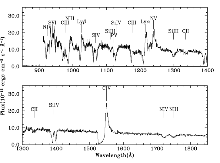
Figure 1.: The calculated spectrum for the fiducial Shlosman & Vitello geometry as observed at an inclination of 62.5^∘ and assuming both the disk and the WD radiate as blackbodies.

Fig. 1 illustrates the results of a typical simulation using parameters that are identical to those of the fiducial model discussed by Shlosman & Vitello at an inclination angle of 62.5^∘. For this and other examples described below, $10^{6}$ photon bundles were created and followed through the wind to create the final spectrum; the spectra cover 1000 Å binned at 0.5 Å intervals. The fiducial model is for a system with a 40,000 K WD with a mass of 0.8 $\>M_{\hbox{$\odot$}}$ and radius of $6\times 10^{8}\rm\>cm$. The disk is presumed to be in a steady state with $\dot{m}_{disk}$ of $\rm 10^{-8}\rm\>\mbox{$\>M_{\hbox{$\odot$}}$}\>yr^{-1}$ and to extend from the WD surface and to 34 R_WD. The wind arises from the disk between 4 and 12 R_WD, and at its inner edge has streamlines that are at 12^∘ with respect to the axis of the system, while at the outer edge the streamlines are 65^∘ with respect to the normal. The scale length for defining the velocity of the wind is 100 R_WD so the wind does not reach terminal velocity until the wind is well outside the system. The terminal velocity along each stream line is 3 times the escape velocity at the footpoint of the wind, so that the most rapidly moving portions of the wind are located at its inner edge. For a more complete description of the kinematic model, see Shlosman & Vitello (1993).

In the simulated spectrum shown in Fig. 1, both disk and the WD spectral distributions have been formed from appropriately weighted blackbodies, so that all of the features in the spectrum are due to the effects of the wind, including the sharp cutoff at 912 Å. In this simulation, C IV shows a well-developed P Cygni profile. Ly$\alpha$ and Ly$\beta$ also show emission wings to their profiles, even though the ionization fraction of H in the outer wind is quite low. O VI is not evident. A number of lower ionization potential lines, such as the Si IV doublet at 1400 Å appear only in absorption. These ions are present only near the disk and as a result we see them only in absorption along the line of sight to the disk.

Figure 2.: The calculated spectrum for the fiducial Shlosman & Vitello geometry, which has $\dot{m}_{disk}$ of $\rm 10^{-8}\rm\>\mbox{$\>M_{\hbox{$\odot$}}$}\>yr^{-1}$ and $\dot{m}_{wind}$ of $\rm 10^{-9}\rm\>\mbox{$\>M_{\hbox{$\odot$}}$}\>yr^{-1}$ as a function of inclination angle. In contrast to Fig. 1, here the disk and WD were simulated in terms of appropriately weighted Hubeny (1988) model atmospheres.

Our C IV profiles differ in detail from those produced by Shlosman & Vitello (1993). In particular we find somewhat wider absorption profiles at moderate inclination angles and somewhat greater emission at high inclination. This is almost surely due to differences in the ionization structure in the two calculations. In the Shlosman & Vitello model calculation, the dominant state of C far from the WD appears to be C V, while our wind retains significant C IV at large radii. It is not clear at this stage which ionization structure is more correct. The implication, if our ionization calculation is more accurate, is that we will require somewhat lower mass loss rates than did Shlosman & Vitello for modelling the spectra of specific CVs.

In Fig. 2, the same model is shown for inclinations ranging from 10^∘ to 80^∘, but in this case the disk and WD are simulated in terms of appropriately weighted stellar atmospheres. At 10^∘, when the observer views the system from “inside” the inner wind cone, the effects of the wind on the spectrum are quite subtle, and nearly all of the features are photospheric with the exception of the narrow emission profiles of Ly$\alpha$ and C IV. At angles of 27.5, 45, and 62.5^∘, the observer is viewing the disk through larger and larger columns of wind material and more ions become apparent. At 62.5^∘, the line of sight skims over the outer lower temperature portion of the disk and therefore more and more low ionization lines appear in the spectrum. Emission becomes more and more important in ions that are extended in the wind, such as C IV and N V, not so much because the flux due to emission has increased, but primarily because the projected size and hence emission from the disk is decreasing. A comparison of the spectrum in Fig. 1 to the 62.5^∘ panel in Fig. 2. shows how important an accurate “photospheric” model of the disk and WD remains in the FUV. Finally, at 80^∘, when the observer views the system from “outside” the wind cone, the spectrum appears dominated by emission lines.

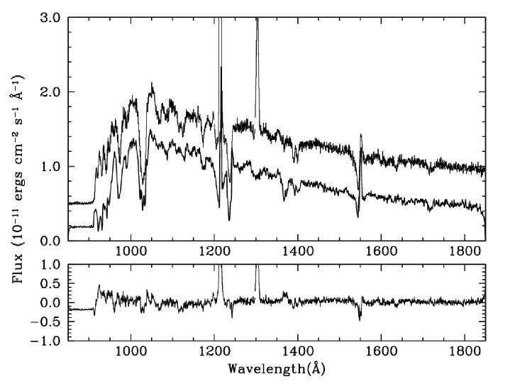
Figure 3.: A comparison between the HUT spectrum of Z Cam and a model spectrum calculated using a prescription for the wind geometry similar to that suggested by Knigge et al. (1997). The model has been smoothed slightly to reflect the resolution of HUT. For clarity, the data have been displaced above the model in the top panel. The strong features at 1216 Å and 1304 Å are air glow lines. The difference between the data and the model is shown in the bottom panel.

3. Comparisons to Spectra of Real CVs

In the absence of a physical model of the wind from a dwarf nova in outburst, any description of a bi-conical flow necessarily has a large number of parameters. It is far from clear exactly how to explore the parameter space, especially since the nature of the boundary layer is unknown in most if not all of the systems involved. Furthermore, given our limited experience at this point, it is not obvious whether more than one wind structure can produce a similar wind spectrum.

However, an example of the type of “fit” that can be obtained is shown in Fig. 3, which shows data obtained with HUT during a normal outburst of Z Cam compared to a model spectrum generated using a wind geometry nearly identical to that described by Knigge et al. (1997). Specifically, the model shown here has the same amount of collimation, the same acceleration length and terminal velocity, as well as the same value of $5\times 10^{-9}\rm\>\mbox{$\>M_{\hbox{$\odot$}}$}$ for $\dot{m}_{disk}$ (originally derived from fitting the continuum spectrum). The model shown is for an inclination of 49^∘, which is in the range allowed for Z Cam . Qualitatively, the model spectrum and the data resemble one another quite well. The strong resonance lines of C IV, N V, and O VI have approximately the right profiles, and many of the features of the lower ionization lines can be seen in both the model and in the data. The main difference between the two models is in $\dot{m}_{wind}$. Knigge et al. (1997) assumed that $\dot{m}_{wind}$ was $5\times 10^{-10}\rm\>\mbox{$\>M_{\hbox{$\odot$}}$}$ and found that ionization fractions of C IV, NV, and O VI were relatively low, a few % or less. We however find a better fit with $\dot{m}_{wind}$ of $1\times 10^{-10}\rm\>\mbox{$\>M_{\hbox{$\odot$}}$}\>yr^{-1}$. The ionization fractions of C IV, N V and O VI are calculated in Python and turn out to be substantial in much of the wind.

4. Summary

The inherent advantages of a Monte Carlo approach in simulating the spectra of cataclysmic variables is the ease with which one can model complex geometries. In the Monte Carlo approach, axially symmetric winds are not significantly more difficult than spherical winds. In the case of Python, we have now progressed to the point of spectral verisimilitude, the point where it is difficult to distinguish a simulation from data. The wind prescriptions required to produce verisimilitude are not that different from those which were developed to model C IV line profiles.

On the other hand, preliminary comparisons of the models and data suggest that considerable work will be required to reproduce the spectra of some dwarf novae. Although we are having some successes, such as the model shown here for Z Cam and with the FUSE spectrum of SS Cygni (Froning et al. 2001), it is quite difficult to reproduce in detail the observed spectra over a broad wavelength range of other CVs, far more difficult than to reproduce an individual line profile. It is not yet clear whether this is due to the fact that we have yet to hit upon the correct parameters in the geometries implemented in Python, or whether more sophisticated treatment of the physics involved in a wind is involved.

To address the former, we are embarking upon an effort to fully explore the parameter space inherent in the existing models and to compare these models to a variety of HUT, FUSE and HST spectra of high state CVs. This should allow us to determine whether there is a single class of models, broadly or narrowly collimated for example, that can be used to approximate the wind geometry in majority of CVs. To address the latter, we are beginning comparisons with models of O star winds for which there is considerable history and expertise. This should provide a clear validation of the code itself and suggest areas where the physics must be improved.

Acknowledgments.

This work was supported by NASA through grant G0-7362 and GO-8279 from the Space Telescope Science Institute, which is operated by AURA, Inc., under NASA contract NAS5-26555.

References

Castor, J. I. & Lamers, H. J. G. L. M. 1979, ApJS, 39, 481

Drew, J. E. 1987, MNRAS, 224, 595

Ferland, G. J. 2000, Revista Mexicana de Astronomia y Astrofisica Conference Series, 9, 153

Froning, C. , Long, K. S., Drew, J. E., Knigge, C., Proga, D., & Mattei, J. A. 2001, these proceedings.

Hartley, L., Drew, J. E., & Long, K. S. 2001, these proceedings

Hubeny, I. 1988, Computer Phys. Comm., 52, 103

Kurucz, R. L. 1991, NATO ASIC Proc. 341: Stellar Atmospheres - Beyond Classical Models, 441

Knigge, C., Long, K. S., Blair, W. P., & Wade, R. A. 1997, ApJ, 476, 291

Knigge, C., Woods, J. A., & Drew, E. 1995, MNRAS, 273, 225

Lucy, L. B. 1999, A&A, 345, 211

Mauche, C. W. & Raymond, J. C. 1987, ApJ, 323, 690

Mazzali, P. A. & Lucy, L. B. 1993, A&A, 279, 447

Shlosman, I., & Vitello, P. 1993, ApJ, 409, 372

Verner, D. A., Verner, E. M., & Ferland, G. J. 1996, Atomic Data and Nuclear Data Tables, 64, 1