GALAXY CLUSTERS IN HUBBLE VOLUME SIMULATIONS: COSMOLOGICAL CONSTRAINTS FROM SKY SURVEY POPULATIONS

Abstract

We use giga-particle N-body simulations to study galaxy cluster populations in Hubble volumes of $\Lambda$CDM ($\Omega_{m}=0.3$, $\Omega_{\Lambda}=0.7$) and $\tau$CDM ($\Omega_{m}=1$) world models. Mapping past light-cones of locations in the computational space, we create mock sky surveys of dark matter structure to $z\!\simeq\!1.4$ over $10,000$ sq deg and to $z\!\simeq\!0.5$ over two full spheres. Calibrating the Jenkins mass function at $z\!=\!0$ with samples of $\sim\!1.5$ million clusters, we show that the fit describes the sky survey counts to $\mathrel{\hbox to0.0pt{\lower 3.0pt\hbox{$\mathchar 536\relax$}\hss}\raise 2.0pt\hbox{$\mathchar 316\relax$}}20\%$ acccuracy over all redshifts for systems more massive than poor galaxy groups ($5\times 10^{13}\hbox{$\,h^{-1}$}{\rm M}_{\odot}$).

Fitting the observed local temperature function determines the ratio $\beta$ of specific thermal energies in dark matter and intracluster gas. We derive a scaling with power spectrum normalization $\beta\!\propto\!\sigma_{8}^{5/3}$, and find that the $\Lambda$CDM model requires $\sigma_{8}\!=\!1.04$ to match $\beta\!=\!1.17$ derived from gas dynamic cluster simulations. We estimate a $10\%$ overall systematic uncertainty in $\sigma_{8}$, $4\%$ arising from cosmic variance in the local sample and the bulk from uncertainty in the absolute mass scale of clusters.

Considering distant clusters, the $\Lambda$CDM model matches EMSS and RDCS X–ray-selected survey observations under economical assumptions for intracluster gas evolution. Using transformations of mass-limited cluster samples that mimic $\sigma_{8}$ variation, we explore Sunyaev–Zel’dovich (SZ) search expectations for a 10 sq deg survey complete above $10^{14}\hbox{$\,h^{-1}$}{\rm M}_{\odot}$. Cluster counts are shown to be extremely sensitive to $\sigma_{8}$ uncertainty while redshift statistics, such as the sample median, are much more stable. Redshift information is crucial to extract the full cosmological diagnostic power of SZ cluster surveys.

For $\Lambda$CDM, the characteristic temperature at fixed sky surface density is a weak function of redshift, implying an abundance of hot clusters at $z>1$. Assuming constant $\beta$, four $kT>8{\rm\ keV}$ clusters lie at $z>2$ and 40 $kT>5{\rm\ keV}$ clusters lie at $z>3$ on the whole sky. Too many such clusters can falsify the model; detection of clusters more massive than Coma at $z>1$ violates $\Lambda$CDM at $95\%$ confidence if their surface density exceeds $0.003$ per sq deg, or 120 on the whole sky.

1. Introduction

Studies of galaxy clusters provide a critical interface between cosmological structure formation and the astrophysics of galaxy formation. Spatial statistics of the cluster population provide valuable constraints on cosmological parameters while multi-wavelength studies of cluster content offer insights into the cosmic mix of clustered matter components and into the interactions between galaxies and their local environments.

In the near future, the size and quality of observed cluster samples will grow dramatically as surveys in optical, X–ray and sub-mm wavelengths are realized. In the optical, the ongoing wide-field 2dF (Colless et al. 2001) and SDSS (Kepner et al. 1999; Nichol et al. 2001; Annis et al. 2001) surveys will map the galaxy and cluster distributions over large fractions of the sky to moderate depth ($z\!\sim\!0.3$), while deeper surveys are probing of order tens of degrees of sky to $z\!\sim\!1$ (Postman et al. 1996; Dalton et al. 1997; Zaritsky et al. 1997; Ostrander et al. 1998; Scoddeggio et al. 1999; Gal et al. 2000; Gladders & Yee 2000; Willick et al. 2001; Gonzalez et al. 2001). In the X–ray, ROSAT archival surveys (Scharf et al. 1997; Rosati et al. 1998; Ebeling et al. 1998; Viklinin et al. 1998; deGrandi et al. 1999; Bohringer et al. 2001; Ebeling, Edge & Henry 2001; Gioia et al. 2001) have generated redshift samples of many hundreds of clusters. Similar surveys to come from developing Chandra and XMM archives (e.g., Romer et al. 2001) will lead to order of magnitude improvements in sample size and limiting sensitivity. Finally, the detection of clusters via their spectral imprint on the microwave background (Sunyaev & Zel’dovich 1972; Birkinshaw 1999) offers a new mode of efficiently surveying for very distant ($z>1$) clusters with hot, intracluster plasma (Barbosa et al. 1996; Holder et al. 2000; Kneissl et al. 2001).

Deciphering the cosmological and astrophysical information in the coming era of large survey data sets requires the ability to accurately compute expectations for observables within a given cosmology. Given some survey observation $R$ at redshift $z$, a likelihood analysis requires the probability $p(R,z\,|\,{\cal C},{\cal A})$ that such data would arise within a model described by sets of cosmological ${\cal C}\!\equiv\!\{C_{i}\}$ and astrophysical ${\cal A}\!\equiv\!\{A_{j}\}$ parameters. Considering clusters as nearly a one-parameter family ordered by total mass $M$, the likelihood of the observable $R$ can be written

$$p(R,z\,|\,{\cal C},{\cal A})\ =\frac{\int dM\ p(M,z\,|\,{\cal C})\ p(R\,|\,M,z,{\cal A})}{\int dM\ p(M,z\,|\,{\cal C})}.$$ (1)

where $p(M,z\,|\,{\cal C})$ is the likelihood that a cluster of mass $M$ exists at redshift $z$ in cosmology ${\cal C}$ within the survey of interest, and $p(R\,|\,M,z,{\cal A})$ is the likelihood that observable $R$ is associated with such a cluster given the astrophysical model ${\cal A}$.

Separating the problem in this way assumes its pieces to be independent. The space density $n(M,z\,|\,{\cal C})$, or mass function, describes the probability of finding a cluster at redshift $z$ with total mass $M$ within comoving volume element $dV$

$$p(M,z\,|\,{\cal C})\ \propto\ n(M,z\,|\,{\cal C})\,dV.$$ (2)

The absence of explicit astrophysical dependence in the mass function is based on the assumption that weakly interacting dark matter dominates the matter energy density. If a cluster’s total mass $M$ is relatively immune to astrophysical processes, then the mass function is well determined by the gravitational clustering of dark matter. On the other hand, the likelihood of a particular observable feature $p(R\,|\,M,z,{\cal A})$, is dependent, often critically, on the astrophysical model. For optical and X–ray observations, it encapsulates the answer to the question “how do dark matter potential wells lights up?”

For Gaussian initial density fluctuation spectra, Press & Schechter (1974; PS) used a spherical collapse argument and $N$-body simulation to show that the space density of the rarest clusters is exponentially sensitive to the amplitude of density perturbations on $\sim 10\hbox{$\,h^{-1}$}{\rm\ Mpc}$ scales. The analytic form of PS was put on a more rigorous footing by Bond et al. (1991), but recent extensions to ellipsoidal collapse (Sheth & Tormen 1999; Lee & Shandarin 1999) revise the original functional form. Calibration by N-body simulations has led to a functional shape for the mass function that retains the essential character of the original PS derivation (Jenkins et al. 2001, hereafter J01, and references therein). For cluster masses defined using threshold algorithms tied to the cosmic mean mass density $\hbox{$\bar{\rho}_{m}$}(z)$, J01 show that the mass fraction in collapsed objects is well described by a single function that depends only on the shape of the filtered power spectrum of initial fluctuations $\sigma^{2}(M)$.

Complications arise in determining the mass function $n(M,z)$ from both simulations and observations. The first is semantic. Clusters formed from hierarchical clustering do not possess unique, or even distinct, physical boundaries, so it is not obvious what mass to assign to a particular cluster. This issue is solvable by convention, and we choose here a commonly employed measure $M_{\Delta}$, defined as the mass interior to a sphere within which the mean interior density is a fixed multiple $\Delta$ of the critical density $\hbox{$\rho_{c}$}(z)$ at the epoch of identification $z$. Acknowledging the non-unique choice of threshold, we develop in an appendix a model, based on the mean density profile of clusters derived from simulations (Navarro, Frenk & White 1996; 1997), that transforms the mass function fit parameters to threshold values different from that used here.

Attempts to empirically constrain the mass function are complicated by the inability to directly observe the theoretically defined mass. Instead, a surrogate estimator $\hat{M}$ must be employed that is, in general, a biased and noisy representation of $M_{\Delta}$. For example, estimates derived from the weak gravitational lensing distortions induced on background galaxies tend to overestimate $M_{\Delta}$ by $\!\sim\!20\%$, with a dispersion of order unity (Metzler, White & Loken 2001; White, van Waerbeke & Mackey 2001)).

The temperature $T$ of the intracluster medium (ICM) derived from X–ray spectroscopy is an observationally accessible mass estimator. Gas dynamic simulations predict that the ICM rarely strays far from virial equilibrium (Evrard 1990; Evrard, Metzler & Navarro 1996; Bryan & Norman 1998; Yoshikawa, Jing & Suto 2000; Mathiesen & Evrard 2001), so that $p(M\,|\,T)$ is well described by a mean power–law relation with narrow ($\mathrel{\hbox to0.0pt{\lower 3.0pt\hbox{$\mathchar 536\relax$}\hss}\raise 2.0pt\hbox{$\mathchar 316\relax$}}15\%$ in mass) intrinsic scatter. Observations are generally supportive of this picture (Hjorth, Oukbir & van Kampen 1998; Mohr, Mathiesen & Evrard 1999; Horner et al. 1999; Nevalainen et al. 2000), but the detailed form of $p(M\,|\,T)$ remains uncertain. The overall normalization is a particular concern; we cannot prove that we know the median mass of, say, a $6{\rm\ keV}$ cluster to better than $25\%$ accuracy.

Even with this degree of uncertainty, the space density of clusters as a function of $T$ (the temperature function) has been used to place tight constraints on $\sigma_{8}$, the present, linear-evolved amplitude of density fluctuations averaged within spheres of radius $8\hbox{$\,h^{-1}$}{\rm\ Mpc}$. Henry & Arnaud (1991) derived $\sigma_{8}\!=\!0.59\pm 0.02$ from temperatures of 25 clusters in a bright, X–ray flux limited sample, assuming $\Omega_{m}\!=\!1$. Subsequent analysis of this sample (White, Efstathiou & Frenk 1993; Eke, Cole & Frenk 1996; Vianna & Liddle 1996; Fan, Bahcall & Cen 1997; Kitayama & Suto 1997; Pen 1998) and revised samples (Markevitch 1998; Blanchard et al. 2000) generated largely consistent results and extended constraints to arbitrary $\Omega_{m}$. For example, Pierpaoli, Scott & White (2001), reanalyzing the Markevitch sample using revised temperatures of White (2000), find

$$\sigma_{8}\ =\ 0.495\,^{+0.034}_{-0.037}\ \ \Omega_{m}^{-0.60}.$$ (3)

Accurate determination of $\sigma_{8}$ is a prerequisite for deriving constraints on the clustered mass density $\Omega_{m}$ from a differential measurement of the local and high redshift cluster spatial abundances. Most studies have excluded the possibility that $\Omega_{m}\!=\!1$ from current data (Luppino & Kaiser 1997; Bahcall, Fan & Cen 1997; Carlberg, Yee & Ellingson 1997; Donahue et al. 1998; Eke et al. 1998; Bahcall & Fan 1998) but others disagree (Sadat, Blanchard & Oukbir 1998; Blanchard & Barlett 1998; Vianna & Liddle 1999). Uncertainty in $\sigma_{8}$ plays a role in this ambiguity, as recently illustrated by Borgani et al. (1999a). In their analysis of 16 CNOC clusters at redshifts $0.17\leq z\leq 0.55$, the estimated value of $\Omega_{m}$ shifts by a factor 3, from $0.35$ to $1.05$, as $\sigma_{8}$ is varied from $0.5$ to $0.6$.

Motivated by the need to study systematic effects in both local and distant cluster samples, we investigate the spatial distribution of clusters in real and redshift space samples derived from $N$-body simulations of cosmic volumes comparable in scale to the Hubble Volume $(c/{\rm H_{0}})^{3}$. A pair of $10^{9}$ particle realizations of flat cold, dark matter (CDM) cosmologies are evolved with particle mass equivalent to that associated with the extended halos of bright galaxies. The simulations are designed to discover the rarest and most massive clusters (by maximizing volume) while retaining force and mass resolution sufficient to determine global quantities (mass, shape, low-order kinematics) for objects more massive than poor groups of galaxies ($\sim\!5\times 10^{13}\hbox{$\,h^{-1}$}{\rm M}_{\odot}$). To facilitate comparison to observations, we generate output that traces the dark matter structure along the past light-cone of two observing locations within the computational volume. These virtual sky surveys, along with usual fixed proper time snapshots, provide samples of millions of clusters that enable detailed statistical studies. We publish the cluster catalogs here as electronic tables.

In this paper, we extend the detailed cluster mass function analysis of J01 to the sky survey output, updating results using a cluster finding algorithm with improved completeness properties for poorly resolved groups. We match the observed local X–ray temperature function by tuning the proportionality factor $\beta$ between the specific energies of dark matter and intracluster gas. The required value of $\beta$ depends on the assumed $\sigma_{8}$, and we derive a scaling $\beta\!\sim\!\sigma_{8}^{5/3}$ based on virial equilibrium and the Jenkins’ mass function form. From $z\!=\!0$ subvolumes sized to local temperature samples, we show that sample variance of temperature-limited samples contributes $\sim\!4\%$ uncertainty to determinations of $\sigma_{8}$. Uncertainty in converting temperatures to masses remains the dominant source of systematic error in $\sigma_{8}$, and we investigate the influence of a $25$ per cent uncertainty in mass scale on expectations for Sunyaev-Zel’dovich searches.

In §2, we describe the simulations, including the process of generating sky survey output, and the model used to convert dark matter properties to X–ray observables. The cluster mass function is examined in §3. Million cluster samples at $z\!=\!0$ are used to determine the best fit parameters of the Jenkins mass function, and we show that this function reproduces well the sky survey populations extending to $z\!>\!1$. The interplay between the fit parameters, $\sigma_{8}$ and the normalization of cluster masses is explored, and this motivates a procedure for transforming the discrete cluster sets to mimic variation in $\sigma_{8}$.

In §4, we use observations analyzed by Pierpaoli et al. to calibrate the specific energy factor $\beta$ for each model. We explore properties of the high redshift cluster population in §5, emphasizing uncertainties from $\sigma_{8}$ error, intracluster gas evolution and possible X–ray selection biases under low signal-to-noise conditions. The $\sigma_{8}$ transformations developed in §3 are used to explore cluster yields anticipated from upcoming SZ surveys, and the median redshift in mass-limited samples is identified as a robust cosmological discriminant. Characteristic properties of the $\Lambda$CDM cluster population are summarized in §6, and we review our conclusions in §7.

2. Hubble Volume Simulations

Table 1Model Parameters.

Model	$\Omega_{m}$	$\Omega_{\Lambda}$	$\sigma_{8}$	$z_{init}$	$L$	$m$
$\Lambda$CDM	0.3	0.7	0.9	35	3000	$2.25$
$\tau$CDM	1.0	0	0.6	29	2000	$2.22$

After an upgrade in 1997 of the Cray T3E at the Rechenzentrum Garching to 512 processors and 64Gb of memory, we carried out a pair of one billion ($10^{9}$) particle simulations over the period Oct 1997 to Feb 1999. A memory-efficient version of Couchman, Pearce and Thomas’ Hydra N-body code (Pearce & Couchman 1997) parallelized using shmem message-passing utilities was used to perform the computations. MacFarland et al. (1998) provide a description and tests of the parallel code.

We explore two cosmologies with a flat spatial metric, a $\Lambda$CDM model dominated by vacuum energy density (a non-zero cosmological constant) and a $\tau$CDM model dominated by non-relativistic, cold dark matter. The $\tau$CDM model completed May 1998 while the $\Lambda$CDM model finished Feb 1999. Published work from these simulations includes an extensive analysis of counts-in-cells statistics (to $>10^{\rm th}$ order) by Colombi et al. (2000) and Szapudi et al. (2000), investigation of the clustering behavior of clusters (Colberg et al. 2000; Padilla & Baugh 2001), analysis of two-point function estimators (Kerscher, Szapudi & Szalay 2000), a description of the mass function of dark matter halos (J01), a study of confusion on the X–ray sky due to galaxy clusters (Voit, Evrard & Bryan 2001), and statistics of pencil–beam surveys (Yoshida et al. 2000). Kay, Liddle & Thomas (2001) use the sky survey catalogs to predict Sunyaev–Zel’dovich (SZ) signatures for the planned Planck Surveyor mission while Outram et al. (2001) use the deep mock $\Lambda$CDM surveys to test analysis procedures for the 2dF QSO Redshift Survey.

2.1. Simulation description

Table 1 summarizes parameter values for each model, including the final epoch matter density $\Omega_{m}$, vacuum energy density $\Omega_{\Lambda}$, power spectrum normalization $\sigma_{8}$, starting redshift $z_{init}$, simulation side length $L$ and particle mass $m$.

Values of $\sigma_{8}$ were chosen to agree approximately with both the amplitude of temperature anisotropies in the cosmic microwave background as measured by COBE and with the nearby space density of rich X–ray clusters. The degree of uncertainty in these constraints allows the final space density of clusters as a function of mass to differ between the two simulations. However, as we discuss below, it is possible to ensure that the observed space density of clusters as a function of X–ray temperature is matched in both models by adjusting a free factor $\beta$ used to link X-ray temperature to dark matter velocity dispersion.

To initiate the numerical experiments, particle positions and momenta at $z_{init}$ are generated by perturbing a replicated ‘glass’ of one million particles with a set of discrete waves randomly drawn from power spectra computed for each cosmology. Initial Fourier modes of the applied perturbations have amplitudes drawn from a Gaussian distribution with variance given by the power spectrum $P(k)\!=\!T(k)P_{\rm prim}(k)$. A Harrison–Zel’dovich primordial spectrum $P_{\rm prim}(k)\!\propto\!k$ is assumed for both models. For the $\Lambda$CDM model, the transfer function $T(k)$ is computed using CMBFAST (Seljak & Zaldarriaga 1996) assuming $h=0.7$ and baryon density $\Omega_{b}h^{2}=0.0196$ (Burles & Tytler 1998). The $\tau$CDM model uses transfer function $T(k)=(1+\big{[}aq+(bq)^{3/2}+(cq)^{2}\big{]}^{\nu})^{-1/\nu}$, where $q=k/\Gamma$, $\Gamma\!=\!\Omega_{m}h$, $a=6.4\hbox{$\,h^{-1}$}{\rm\ Mpc}$, $b=3\hbox{$\,h^{-1}$}{\rm\ Mpc}$, $c=1.7\hbox{$\,h^{-1}$}{\rm\ Mpc}$ and $\nu=1.13$ (Bond & Efstathiou 1984).

The simulations are designed to resolve the collapse of a Coma-sized cluster with 500 particles. Although this resolution is sufficient to capture only the later stages of the hierarchical build-up of clusters, convergence tests (Moore et al. 1998; Frenk et al. 1999) show that structural properties on scales larger than a few times the gravitational softening length are essentially converged. From tests presented in J01 and in an Appendix to this work, cluster identification is robust down to a level of about $20$ particles. Using $M_{\rm Coma}\!=\!1.1\times 10^{15}\hbox{$\,h^{-1}$}{\rm M}_{\odot}$ (White et al. 1993), leads to particle mass $2.2\times 10^{12}\hbox{$\,h^{-1}$}{\rm M}_{\odot}$ in both models, comparable to the total mass within $\sim\!300\hbox{$\,h^{-1}$}{\rm\ kpc}$ of bright galaxies (Fischer et al. 2000; Smith et al. 2001; Wilson et al. 2001). The mass associated with one billion particles at the mean mass density sets the length $L$ of the periodic cube used for the computations, resulting in a Hubble Length $L\!=\!c/{\rm H_{0}}\!=\!3\hbox{$\,h^{-1}$}{\rm\ Gpc}$ for the $\Lambda$CDM model and $L=2\hbox{$\,h^{-1}$}{\rm\ Gpc}$ for $\tau$CDM.

A Newtonian description of gravity is assumed, appropriate for weak-field structures. A non-retarded gravitational potential is employed because the peculiar acceleration converges on scales well below the Hubble length. The good agreement between the higher-order clustering statistics of the simulations and expectations derived from an extended perturbation theory treatment of mildly non-linear density fluctuations provides indirect evidence that this treatment of gravity is accurate (Colombi et al. 2000; Szapudi et al. 2000).

Gravitational forces on each particle are calculated as a sum of a long-range component, determined on a uniform spatial grid of $1024^{3}$ elements using Fast Fourier Transforms, and a short-range component found by direct summation. The latter force is softened with a spline-smoothing roughly equivalent to a Plummer law gravitational potential $\phi(r)\!\propto\!(r^{2}+\varepsilon^{2})^{-1/2}$ with smoothing scale $\varepsilon\!=\!0.1\hbox{$\,h^{-1}$}{\rm\ Mpc}$. A leapfrog time integration scheme is employed with 500 equal time steps for each calculation.

Table 2Light-cone Sky Surveys.

Name	center	solid angle	$z_{\rm max}$ ($\Lambda$)	$z_{\rm max}$ ($\tau$)
MS	$(L/2,L/2,L/2)$	$4\pi$	0.57	0.42
VS	$(0,0,0)$	$4\pi$	0.57	0.42
PO	$(0,0,0)$	$\pi/2$	1.46	1.25
NO	$(L,L,L)$	$\pi/2$	1.46	1.25
DW	$(0,0,0)$	$10^{\circ}\times 10^{\circ}$	4.4	4.6
XW	$(0,0,0)$	$16^{\circ}\times 76^{\circ}$	$6.8$	$-$

Processor time for these computations was minimized by employing a parallel algorithm well matched to the machine architecture (MacFarland et al. 1998) and by simulating large volumes that entail a minimum of message passing overhead. The Cray-T3E offers high interprocessor communication bandwidth along with a native message-passing library (shmem) to control data flow. A two-dimensional, block-cyclic domain decomposition scheme allocates particles to processors. Each processor advances particles lying within a disjoint set of rectangular regions of dimension $L\times(L/32)\times(L/16)$ that subdivide the computational space. Each calculation required approximately 35,000 processor hours, or three days of the 512-processor machine. This corresponds to advancing roughly 4000 particles per second on an average step. The computations were essentially limited by I/O bandwidth rather than cpu speed. Execution was performed in roughly twenty stages spanning a calendar time of three to four months, with data archived to a mass storage system between stages. Approximately 500 Gb of raw data were generated by the pair of simulations.

2.2. Sky survey output

In addition to the traditional simulation output of snapshots of the particle kinematic state at fixed proper time, we introduce here sky survey output that mimics the action of collecting data along the past light-cone of hypothetical observers located within the simulation volume. The method extends to wide-angle surveys an approach pioneered by Park & Gott (1991) in simulating deep, pencil-beam observations. Since there is no preferred location in the volume, we chose two survey origins, located at the vertex and center of the periodic cube for convenience.

In a homogeneous world model, a fixed observer at the present epoch $t_{0}$ receives photons emitted at $t<t_{0}$ that have traversed comoving distances $r(t)\ =c\int_{t}^{t_{0}}dt\,a^{-1}(t)$ where $a(t)$ is the scale factor of the metric ($a(t_{0})\!=\!1$) and $c$ the speed of light. The set of events lying along the continuum of concentric spheres $\{t,\vec{r}(t)\}$ for $t<t_{0}$ defines the past light-cone of that observer. In the discrete environment of the numerical simulation, we construct the light-cone survey by choosing spherical shells of finite thickness such that each particle’s state is saved at a pair of consecutive timesteps that bound the exact time of intersection of the light-cone with that particle’s trajectory. Defining $t_{i}$ as the proper time at step $i$ of the computation, we choose inner and outer radii $(1-\eta)r(t_{i+1})$ and $(1+\eta)r(t_{i-1})$. Here $\eta\!\simeq\!0.02$ is a small parameter that safeguards against a particle appearing only once in the output record due to peculiar motion across the discrete shells during a step. The inner radius is set to zero on the final two steps of the computation.

With successive states for particles in the output record, a linear interpolation is performed to recover the original second-order time accuracy of the leap-frog integrator. Given a particle’s position relative to the survey origin $\vec{x}_{i}$ and, at the subsequent step, $\vec{x}_{i+1}\!\equiv\!\vec{x}_{i}+\Delta\vec{x}$, we solve for interpolation parameter $\alpha$ defining position $\vec{x}\!=\!\vec{x}_{i}+\alpha\Delta\vec{x}_{i}$ such that $|\vec{x}|=r(t_{i}+\alpha\Delta t)$, with $\Delta t$ the timestep. For a spherical survey, this implies

$$\alpha\ =\ \frac{r^{2}(t_{i})-x_{i}^{2}}{2(\vec{x_{i}}^{.}\Delta\vec{x}+r(t_{i})\Delta r)}$$ (4)

with $\Delta r\!=\!r(t_{i})-r(t_{i+1})>0$. After solving for $\alpha$, the particle’s position and velocity are interpolated and the result stored to create the processed sky survey data sets. Comoving coordinates and physical velocities are stored as two-byte integers, sufficient to provide $\sim\!\varepsilon/10$ positional accuracy and km/s accuracy in velocity. Data are stored in binary form in multiple files, each covering a spatial subcube of side $L/16$ of the entire computational volume.

The scale $L$, along with the comoving distance–redshift relations shown in Figure 1, determine the redshift extents of the surveys listed in Table 2. Two principal survey types — spheres and octants — extend to distances $L/2$ and $L$, respectively. From the cube center, the MS full-sphere surveys extend to redshifts $z_{\rm max}\!=\!0.57$ ($\Lambda$CDM) and $0.42$ ($\tau$CDM). From the origin and its diagonally opposite image, octant surveys (PO and NO, respectively) extend to redshifts $1.46$ ($\Lambda$CDM) and $1.25$ ($\tau$CDM). The surveys have opposite orientation; both view the interior region of the computational space. The VS sphere centered on the origin is created using translational symmetries of separate octant surveys conducted from the eight vertices of the fundamental cube. The interior portions of the PO and NO surveys are thus subsets (opposite caps) of the VS survey. The combined volumes of the spheres and octants sample the computational volume roughly once for each type. In terms of cosmic time, the octants extend over the last 74% and 71% of the age of the universe ($\Lambda$CDM and $\tau$CDM, respectively), equivalent to roughly a 10 Gyr look-back time.

In addition to these surveys, smaller solid angle wedge surveys reach to greater depth. A $10\times 10$ sq deg deep wedge (DW) extends along the cube diagonal to the opposite corner and reaches redshifts $4.4$ ($\Lambda$CDM) and $4.6$ ($\tau$CDM). For the $\Lambda$CDM model only, a $16\times 76$ sq deg extended wedge (XW) uses periodic images of the fundamental cube to reach $z_{\rm max}\!=\!6.8$. This wedge is a partial extension of the PO survey.

2.3. Connecting to X–ray observations

Connecting to observations of clusters requires a model that relates luminous properties to the underlying dark matter. We focus here on the ICM temperature $T$ under the assumption that both $T$ and the dark matter velocity dispersion $\sigma_{v}$ are related to the underlying dark matter gravitational potential through the virial theorem (Cavaliere & Fusco-Femiano 1976). Empirical support for this assumption comes from the observation that $\hbox{$T$}\!\sim\!\hbox{$\sigma_{\rm gal}$}^{2}$ (e.g., Wu, Xue & Fang 1999), the scaling expected if both galaxies and the ICM are thermally supported within a common potential. High resolution simulations of galaxy formation within a cluster indicate that $\sigma_{\rm gal}$ should accurately reflect the dark matter $\sigma_{v}$ except for the brightest, early-type galaxies which display a mild bias toward lower velocity dispersion (Springel et al. 2000).

Rather than map $T$ to $M$ directly, we prefer to use a one-to-one mapping between $T$ and dark matter velocity dispersion $\sigma_{v}$. This approach has the advantage of naturally building in scatter between $T$ and $M$ at a fractional amplitude $\sim\!10\%$ that is consistent with expectations from direct, gas dynamic modeling (e.g., Mathiesen & Evrard 2001; Thomas et al. 2001). Define a one-dimensional velocity dispersion $\sigma_{v}$ by

$$\hbox{$\sigma_{v}$}^{2}\ =\ \frac{1}{3N_{p}}\ \sum_{i=1}^{N_{p}}\sum_{j=1}^{3}\ |v_{i,j}-\bar{v_{j}}|^{2}$$ (5)

where the index $i$ ranges over the $N_{p}$ cluster members identified within $r_{\Delta}$, $j$ sums over principal directions, and $\bar{v}$ is the mean cluster velocity defined by the same $N_{p}$ members. We assume that $\hbox{$\sigma_{v}$}^{2}$ maps directly to X–ray temperature and introduce as an adjustable parameter the ratio of specific energies $\beta\!\equiv\!\hbox{$\sigma_{v}$}^{2}/(k\hbox{$T$}/\mu m_{p})$, where $k$ is Boltzmann’s constant, $\mu$ the mean molecular weight of the plasma (taken to be $0.59$) and $m_{p}$ the proton mass. We fit $\beta$ by requiring that the models match the local temperature function.

Varying the power spectrum normalization $\sigma_{8}$ leads to shifts in the space density of clusters as a function of mass and velocity dispersion. Values of $\beta$ required to fit X–ray observations thus depend on $\sigma_{8}$, and we derive an approximate form for this dependence in §4.4 below.

3. Cluster Populations

We begin this section by visualizing the evolution of clustering in the octant surveys. Details of the cluster finding algorithm are then presented, and fits to the $z\!=\!0$ mass functions performed for $\Delta\!=\!200$. A simple model for evolving the fit parameters with redshift in the $\Lambda$CDM case is given, and predictions based on the $z\!=\!0$ fits compared to the sky survey output in three broad redshift intervals.

Additional details are provided in two appendices. Appendix A compares output of the SO algorithm employed here to that used by J01. Appendix B presents a model for extending the mass function fits under variation of the density threshold $\Delta$. More generally, it provides a means to transform the discrete cluster sample under variation of $\sigma_{8}$. Appendix C presents the sky survey and $z\!=\!0$ cluster catalogs as electronic tables. Truncated versions in the print edition list the ten most massive clusters in each survey. Electronic versions list all clusters above a mass limit of $5\times 10^{13}\hbox{$\,h^{-1}$}{\rm M}_{\odot}$ (22 particles).

3.1. Evolution of the matter distribution

In Figure 2, we present maps of the Lagrangian smoothed mass density in slices through the octant surveys that extend to $z\!=\!1.25$. Horizontal and vertical maps show comoving and redshift space representations, respectively. Since the Hubble Length far exceeds the characteristic clustering length of the mass, the feature most immediately apparent in the density maps is their overall homogeneity. Gravitational enhancement of the clustering amplitude over time is evident from the fact that the density fluctuations are more pronounced near the survey origin (vertex of each triangular slice) compared to the edge. The effect is subtle in this image because the dynamic range in density, from black to white, spans three orders of magnitude, much larger than the linear growth factors of $1.8$ ($\Lambda$CDM) and $2.2$ ($\tau$CDM) for large-scale perturbations in the interval shown.

To verify the accuracy of the clustering evolution in the octant surveys, we show in Figure 3 the behavior of the rms amplitude of density fluctuations $\langle\delta^{2}\rangle^{1/2}$, where $\delta\!\equiv\!\rho/\hbox{$\bar{\rho}_{m}$}(z)-1$, within spheres encompassing, on average, a mass of $2.2\times 10^{15}\hbox{$\,h^{-1}$}{\rm M}_{\odot}$ (1000 particles). Points in the figure show $\langle\delta^{2}\rangle^{1/2}$ determined by randomly sampling locations within twenty radial shells of equal volume in the octant surveys. Values are plotted at the volume-weighted redshift of each shell. Solid lines are not fits, but show the expectations for $\langle\delta^{2}\rangle^{1/2}$ based on linear evolution of the input power spectrum. Deviations between the measured values and linear theory, shown in the upper panels of Figure 3, are at the $1\%$ level. Although we do not attempt here to model these deviations explicitly, Szapudi et al. (2000) show that the higher-order clustering properties of these simulations at the final epoch are well described by an extended perturbation theory treatment of fluctuation evolution.

Table 3Fit parameters for $\hbox{$\ln\sigma^{-1}$}(M)$.

Model	$\sigma_{15}$	$a$	$b$
$\Lambda$CDM	0.578	0.281	0.0123
$\tau$CDM	0.527	0.267	0.0122

The orientation of the slice shown in Figure 2 is chosen to include the most massive cluster in the $\Lambda$CDM octant surveys. It lies at the surprisingly high redshift $z\!=\!1.04$. The inset of Figure 2b shows that this cluster is actively forming from mergers fed by surrounding filaments. In Figure 4, we show a close-up of the redshift space structure in $75,000\hbox{ km s${}^{-1}$}$ wide regions centered at $z\!=\!1.1$ and lying just interior to the vertical edges of the redshift-space views of Figure 2. The grey-scale shows only overdense material $\delta>0$ and the region includes the most massive $\Lambda$CDM cluster. With rest-frame line-of-sight velocity dispersion $1964\hbox{ km s${}^{-1}$}$,it produces a $\sim 16,000\hbox{ km s${}^{-1}$}$ sized ‘finger-of-God’ feature in the lower right image.

Along with this extreme object, close inspection of Figure 4 reveals many more smaller fingers representing less massive clusters in the $\Lambda$CDM image. The $\tau$CDM panel contains many fewer such clusters. It is this difference that motivates high redshift cluster counts as a sensitive measure of the matter density parameter $\Omega_{m}$. To perform quantitative analysis of the cluster population, we first describe the method used to identify clusters in the particle data sets.

3.2. Cluster finding algorithm

A number of methods have been developed for identifying clusters within the particle data sets of cosmological simulations. We refer the reader to J01, White (2000) and Lacey & Cole (1994) for discussion and intercomparisons of common approaches. Two algorithms are employed by J01. One is a percolation method known as “friends-of-friends” (FOF) that identifies a group of particles whose members have at least one other group member lying closer than some threshold separation. The threshold separation, typically expressed as a fraction $\eta$ of the mean interparticle spacing, is a parameter whose variation leads to families of groups, referred to as FOF($\eta$), with favorable nesting properties (Davis et al. 1985).

The other algorithm of J01 is a spherical overdensity (SO) method that identifies particles within spheres, centered on local density maxima, having radii defined by a mean enclosed iso-density condition. We use here an SO algorithm that differs slightly from that of J01. The iso-density condition requires the mean mass density within radius $r_{\Delta}$ to be a factor $\Delta$ times the critical density $\hbox{$\rho_{c}$}(z)$ at redshift $z$. J01 define spherical regions that are overdense with respect to the mean background, rather than critical, mass density. For clarity, we refer to the approaches as ‘mean SO’ and ‘critical SO’ algorithms. If not stated explicitly, reference to SO($\Delta$) should be read as the critical case evaluated at contrast $\Delta$. By definition, a critical SO($\Delta$) population is identical to a mean SO($\hbox{$\Delta$}/\Omega_{m}$) population.

Our method employs a code independent of that used by J01. The codes produce matching output for well-resolved groups, but differ at low particle number. Appendix A provides a discussion of completeness based on direct comparison of group catalogs from the algorithms.

3.3. Mass function fits at $z\!=\!0$

By coadding 22 snapshots of 11 Virgo Consortium simulations ranging in scale from $84.5\hbox{$\,h^{-1}$}{\rm\ Mpc}$ to $3000\hbox{$\,h^{-1}$}{\rm\ Mpc}$, J01 showed that the space density of clusters defined by either FOF(0.2) or SO(180) algorithms are well described by a single functional form when expressed in terms of $\hbox{$\ln\sigma^{-1}$}(M)$, where $\sigma^{2}(M)$ is the variance of the density field smoothed with a spherical top-hat filter enclosing mass $M$ at the mean density. Define the mass fraction $f(\hbox{$\ln\sigma^{-1}$})$ by

$$f(\hbox{$\ln\sigma^{-1}$})\ \equiv\ \frac{M}{\hbox{$\bar{\rho}_{m}$}(z)}{{\rm d}n(<M,z)\over\hbox{$\hbox{\rm d$\,$ln }\sigma^{-1}$}}$$ (6)

with $\hbox{$\bar{\rho}_{m}$}(z)$ the background matter density at the epoch of interest and $n(<M,z)$ the cumulative number density of clusters of mass $M$ or smaller. The general form found by J01 for the mass function is

$$f(\hbox{$\ln\sigma^{-1}$})\ =\ A\,\exp\big{[}-|\ln\sigma^{-1}+B\,|^{\epsilon}\big{]}$$ (7)

where $A$, $B$ and $\epsilon$ are fit parameters. The amplitude $A$ sets the overall mass fraction in collapsed objects, $e^{B}$ plays the role of a (linearly evolved) collapse perturbation threshold, similar to the parameter $\delta_{c}$ in the Press-Schechter model or its variants, and $\epsilon$ is a stretch parameter that provides the correct shape of the mass function at the very dilute limit.

Values of these parameters depend on the particular cluster finding scheme implemented, but J01 show them to be independent of cosmology and redshift when cluster masses are based on algorithms tied to the mean mass density. For the FOF(0.2) group catalogs, J01 find that $A\!=\!0.315$, $B\!=\!0.61$ and $\epsilon\!=\!3.8$ provide a fit that describes all of the numerical data to $\mathrel{\hbox to0.0pt{\lower 3.0pt\hbox{$\mathchar 536\relax$}\hss}\raise 2.0pt\hbox{$\mathchar 316\relax$}}20\%$ precision over eight orders of magnitude in number density.

We fit here the SO mass function by employing a quadratic relation describing the filtered power spectrum shape

$$\hbox{$\ln\sigma^{-1}$}(M)\ =\ -\ln\sigma_{15}+a\,\hbox{$\ln M$}+b\,(\hbox{$\ln M$})^{2}$$ (8)

where $M$ is mass in units of $10^{15}\hbox{$\,h^{-1}$}{\rm M}_{\odot}$ and the rms fluctuation amplitude $\sigma_{15}$ at that mass scale is simply related to the fiducial power spectrum normalization by $\ln\sigma_{15}\!=\!\ln(\sigma_{8})+const$. Table 3 lists parameters of the fit to equation (8). The maximum error in the fit is $2\%$ in $\ln\sigma^{-1}$ for masses above $10^{13}\hbox{$\,h^{-1}$}{\rm M}_{\odot}$. For both models, the effective logarithmic slope,

$$\alpha_{\rm eff}(M)\ \equiv\ \hbox{$\hbox{\rm d$\,$ln }\sigma^{-1}$}(M)/\hbox{$\hbox{\rm d$\,$ln }\!M$}\ =\ a+2b\,\hbox{$\ln M$},$$ (9)

slowly varies between $0.2$ and $0.3$ for masses in the range $10^{13}$ to $10^{15.5}\hbox{$\,h^{-1}$}{\rm M}_{\odot}$. The Jenkins mass function (JMF) expression for the differential number density as a function of mass and redshift

$$\hbox{$n_{\rm JMF}$}(M,z)=\frac{A\hbox{$\bar{\rho}_{m}$}(z)}{M}\alpha_{\rm eff}(M)\exp\big{[}-|\hbox{$\ln\sigma^{-1}$}(M)+B|^{\epsilon}\big{]}$$ (10)

is the form that we fit to the simulated cluster catalogs.

Table 4SO(200) mass function parameters.

Model	$A$	$B$	$\epsilon$	$\langle(\delta n/n)^{2}\rangle^{1/2}$
$\Lambda$CDM	0.22	0.73	3.86	0.026
$\tau$CDM	0.27	0.65	3.77	0.028

The critical SO(200) mass functions at $z\!=\!0$ for both models are shown in Figure 5, derived from samples of $1.39$ million ($\Lambda$CDM) and $1.48$ million ($\tau$CDM) clusters above $5\times 10^{13}\hbox{$\,h^{-1}$}{\rm M}_{\odot}$. Fits to equation (10) are shown as dotted lines, with fit parameters listed in Table 4. The upper panels of Figure 5 show the fractional deviations $\delta n/n\!=\!n/n_{JMF}-1$ in bins of width $0.12$ in $\ln M$. Error bars assume Poisson statistics. For bins with 100 or more clusters ($\hbox{$M_{200}$}\mathrel{\hbox to0.0pt{\lower 3.0pt\hbox{$\mathchar 536\relax$}\hss}\raise 2.0pt\hbox{$\mathchar 316\relax$}}2\times 10^{15}\hbox{$\,h^{-1}$}{\rm M}_{\odot}$), the rms deviations $\langle(\delta n/n)^{2}\rangle^{1/2}$ are $\mathrel{\hbox to0.0pt{\lower 3.0pt\hbox{$\mathchar 536\relax$}\hss}\raise 2.0pt\hbox{$\mathchar 316\relax$}}3\%$ (Table 4).

The high statistical precision of these fits is a lower bound on the absolute accuracy of the mass function calibration. Based on the fits performed by J01 to a large ensemble of simulations covering a wider dynamic range in scale than the HV models alone, we estimate that the normalization $A$ may be systematically low by $\sim\!10\%$ (see Appendix A). Considering that this degree of uncertainty in $A$ corresponds to an uncertainty in mass of only $2-3\%$, this level of accuracy is sufficient for the practical purpose of comparing to current and near future observations, for which the level of systematic uncertainty in mass is an order of magnitude larger.

Another estimate of systematic error is provided by comparing our results to the recent large simulations of Bode et al. (2001). Their $1\hbox{$\,h^{-1}$}$ Gpc $\Lambda$CDM simulation assumes identical cosmological parameters to our model, but uses a particle mass and gravitational softening smaller by factors of 30 and 7, respectively. Bode et al. employ a measure of mass within a comoving radius $1.5\hbox{$\,h^{-1}$}{\rm\ Mpc}$; this scale encompasses a critical density contrast of 200 at the present epoch for mass $\hbox{$M_{200}$}\!=\!7.94\times 10^{14}\hbox{$\,h^{-1}$}{\rm M}_{\odot}$. From their Figure 6, the space density of clusters above that mass scale is $10^{-6.6}\!\sim\!2.5\times 10^{-7}h^{3}{\rm\ Mpc}^{-3}$. In our $27h^{-3}{\rm\ Gpc}^{3}$ volume, we find 6499 clusters above this mass limit, implying a space density $2.4\times 10^{-7}h^{3}{\rm\ Mpc}^{-3}$.

Figure 5 shows that the two models do not produce identical mass functions at the present epoch; the $\Lambda$CDM space density is lower by a factor $\!\sim\!4$ than that of $\tau$CDM. Two factors combine to make this difference. The first is that our chosen values of $\sigma_{8}$ straddle the constraint derived from fitting the local X–ray cluster space density, such as that quoted in equation (3). The sense of the differences — the $\Lambda$CDM model has lower amplitude and $\tau$CDM higher, both by about $10\%$ – pushes the models in opposite directions. The second factor is that our choice of fixed critical threshold $\Delta\!=\!200$ leads to smaller masses for $\Lambda$CDM clusters. Previous work has typically employed the lower $\Omega_{m}$–dependent thresholds derived by Eke et al. (1996) from the spherical collapse solutions of Lahav et al. (1991) and Lilje (1992). For $\Omega_{m}\!=\!0.3$, Eke et al. calculate critical threshold $\Delta\!=\!97.2$, leading to masses are larger by a factor $\sim\!1.25$ compared to $\Delta\!=\!200$.

Table 5counts of clusters with $hM_{200}/{\rm M}_{\odot}$ above mass limits.

			$\Lambda$CDM				$\tau$CDM
Survey		$5\times 10^{13}$	$10^{14}$	$10^{15}$		$5\times 10^{13}$	$10^{14}$	$10^{15}$
MS		564,875	178,223	322		377,043	102,742	120
VS		565,886	178,483	285		378,548	103,157	111
PO		255,083	64,608	45		107,900	22,853	10
NO		259,279	64,930	42		108,807	23,216	13
DW		5,238	1,316	1		1,833	411	0
Total		1,504,620	441,833	623		878,356	226,602	231

3.4. Sky survey cluster populations

We define cluster catalogs in the sky survey output using the same SO algorithm applied to the snapshots at fixed proper time. A minor modification for the $\Lambda$CDM model must be made in order to define the threshold $\Delta$ with respect to the epoch-dependent critical mass density $\hbox{$\rho_{c}$}(z)=\hbox{$\rho_{c}$}(0)[\Omega_{m}(1+z)^{3}+\Omega_{\Lambda}]$.

For the choice $\hbox{$\Delta$}\!=\!200$, Table 5 lists counts of clusters identified in the sky survey catalogs above mass limits $5\times 10^{13}$, $10^{14}$ and $10^{15}\hbox{$\,h^{-1}$}{\rm M}_{\odot}$. The lower mass limit corresponds to 22 particles and the maximum redshifts of the catalogs are given in Table 2.

Total counts of $1.5$ and $0.9$ million clusters offer large statistical samples. On the other hand, the small numbers of objects at the most massive end of the spectrum put the finite size of the visible universe into context and provide additional motivation for near-future surveys to define an absolutely complete sample of the largest clusters in the universe. Only a few hundred Coma-like or larger clusters are expected on the sky at all redshifts in either cosmology.

Figure 6 shows redshift-space maps of clusters with $\hbox{$M_{200}$}>10^{14}\hbox{$\,h^{-1}$}{\rm M}_{\odot}$ and $z\leq 1.25$ in $3\times 90$ deg strips taken from the PO octant surveys of the $\tau$CDM (left) and $\Lambda$CDM (right) models. The surveys display markedly different evolution at $z>0.5$; distant clusters are more abundant in the low mass density cosmology (Efstathiou, Frenk & White 1993; Eke, Cole & Frenk 1996; Bahcall Fan & Cen 1997). Within the 3 deg slice — a width equivalent to two Sloan Digital Sky Survey scans — the $\Lambda$CDM model contains 3084 clusters above the $10^{14}\hbox{$\,h^{-1}$}{\rm M}_{\odot}$, half lying beyond $z\!=\!0.70$. The $\tau$CDM model contains 1122 clusters, with median $z\!=\!0.39$.

The sky surface density of clusters within three broad redshift intervals are shown as a cumulative function of mass in Figure 7. The ranges in redshift are chosen to represent three classes of observation: local, $z<0.2$; intermediate, $0.2\leq z<0.5$, and high, $0.5\leq z<1.2$. Counts measured within the octant surveys are shown as points while solid lines show the number expected from integrating the Jenkins mass function $N(>\!M)\!=\!\int_{z_{\rm min}}^{z_{\rm max}}\,dz\,(dV/dz)\,\int_{{\rm ln}M}^{\infty}\,\hbox{$\hbox{\rm d$\,$ln }\!M$}^{\prime}\,\hbox{$n_{\rm JMF}$}(M^{\prime},z)$.

For $\tau$CDM, the integral is performed using the fit parameters determined at $z\!=\!0$ (Table 4). For $\Lambda$CDM, we must recognize the fact that, because $\Omega_{m}(z)$ varies along the light-cone, the fit parameters will evolve with redshift. As $\Omega_{m}$ tends to unity at high redshifts, we expect the parameters to converge to the $\tau$CDM values. Since differences in $A$, $B$ and $\epsilon$ between the two models are small at $z\!=\!0$, we take a simple approach and vary the parameters linearly in $\Omega_{m}$. For example, we assume for $A$ that

$$A(\Omega_{m})\ =\ (1-x)A(1)\,+\,xA(0.3),$$ (11)

where $x\!\equiv\!(1-\Omega_{m})/0.7$ and $A(1)$ and $A(0.3)$ are the $z\!=\!0$ fit parameters for $\tau$CDM and $\Lambda$CDM from Table 4. Similar interpolations are assumed for $B$ and $\epsilon$.

The predictions of this model agree very well with the measured counts in the octant surveys. The model is accurate to $\mathrel{\hbox to0.0pt{\lower 3.0pt\hbox{$\mathchar 536\relax$}\hss}\raise 2.0pt\hbox{$\mathchar 316\relax$}}10\%$ in number for $\Lambda$CDM at all masses and redshifts shown. Similar accuracy is displayed for the $\tau$CDM model at low and intermediate redshifts, but the model systematically underestimates counts in the high redshift interval by $\sim\!25\%$.

Dashed lines in Figure 7 show numbers expected by the Press-Schechter model in its simplest form (see J01 for details). For the $\tau$CDM model, the PS curve tends to underestimate the space density at high masses. For the $\Lambda$CDM model, the use of mass measured within a critical, rather than mean, mass density threshold leads to an offset in mass between the measured counts and PS curves at low redshifts. The offset declines as $\Omega_{m}$ approaches unity, resulting in a relatively good match to the simulated counts in the high redshift interval.

In the $\Lambda$CDM panels, we plot the $\tau$CDM JMF curves as dotted lines for comparison. At low redshifts, the two models exhibit an offset in the direction of $\tau$CDM being overabundant relative to $\Lambda$CDM, a difference already discussed in §3.3 for the $z\!=\!0$ population. In the intermediate redshift interval, this offset is reversed at nearly all masses above the $5\times 10^{13}\hbox{$\,h^{-1}$}{\rm M}_{\odot}$ limit. At high redshifts, the $\Lambda$CDM counts are typically an order of magnitude higher than those of $\tau$CDM.

3.5. Sky survey completeness

Comparison of the octant counts with the JMF expectations provides a measure of the incompleteness of the HV sky catalogs that arises from their finite redshift extent. Figure 8 plots the cumulative sky surface density of clusters above mass limits $5\times 10^{13}$, $3\times 10^{14}$, and $10^{15}\hbox{$\,h^{-1}$}{\rm M}_{\odot}$ as a function of redshift. Points show the sky densities of clusters lying at redshift $z$ or higher with masses above the stated limits (top to bottom, respectively), determined by combining the octant surveys of each model. Lines in the figure show the JMF expectations from integrating equation (10) using the linear evolution of the fit parameters, equation (11).

At Coma mass scales ($>\!10^{15}\hbox{$\,h^{-1}$}{\rm M}_{\odot}$), the catalogs are essentially complete, as fewer than one such object is expected over $\pi$ steradian beyond the survey redshift limit. At $3\times 10^{14}\hbox{$\,h^{-1}$}{\rm M}_{\odot}$, the $\Lambda$CDM model octants are missing $\sim\!100$ clusters expected above $z\!=\!1.5$, implying $\sim\!98\%$ completeness. The $\tau$CDM model at this mass limit is essentially complete; the small discrepancy between the measured and JMF counts at redshifts $z\mathrel{\hbox to0.0pt{\lower 3.0pt\hbox{$\mathchar 536\relax$}\hss}\raise 2.0pt\hbox{$\mathchar 318\relax$}}0.5$ reflects the systematic trend exhibited in the high redshift panel of Figure 7. At the mass scale of groups, $5\times 10^{13}\hbox{$\,h^{-1}$}{\rm M}_{\odot}$, the incompleteness becomes more significant. In the $\Lambda$CDM model, for example, $\sim 15\%$ of the group population should lie at $z>1.5$.

The $\Lambda$CDM model possesses a healthy population of very high redshift clusters. Across the whole sky, a cluster as massive as Coma is expected at redshifts as high as $1.3$. At $z>2.5$, one $3\times 10^{14}\hbox{$\,h^{-1}$}{\rm M}_{\odot}$ cluster should lie somewhere on the sky, joined by $\sim\!20,000$ others above $5\times 10^{13}\hbox{$\,h^{-1}$}{\rm M}_{\odot}$, nearly one per square degree. Before getting carried away by such seemingly firm predictions, we must investigate the effect of varying a degree of freedom that has so-far been kept fixed in the models: the amplitude of the fluctuation power spectrum $\sigma_{8}$.

4. The Temperature Function, Absolute Mass Scale and Power Spectrum Normalization Uncertainty

In this section, we use the freedom in the mass-temperature relation to tune $\beta$, the ratio of specific energies in dark matter and ICM gas, so that both models match the observed local temperature function. We show how $\beta$ should scale with $\sigma_{8}$ so as to maintain consistency with observations. The final snapshots are used to calibrate the level of uncertainty in $\sigma_{8}$ arising from sample variance in local volumes. We discuss the overall systematic error in $\sigma_{8}$, then examine in §5 how this uncertainty affects predictions for the high redshift cluster population.

4.1. Fitting local temperature observations

Pierpaoli, Scott & White (2001, hereafter PSW) provide the most recent study of the local temperature function and its constraints on $\sigma_{8}$. The sample of 38 clusters used in their analysis is adapted from the X–ray flux-limited sample of Markevitch (1998) and is designed as an essentially volume-limited sample within redshifts $0.03<z<0.09$ and galactic latitude $|b|>20^{\circ}$ for clusters with $k\hbox{$T$}\mathrel{\hbox to0.0pt{\lower 3.0pt\hbox{$\mathchar 536\relax$}\hss}\raise 2.0pt\hbox{$\mathchar 318\relax$}}6{\rm\ keV}$. PSW update temperatures for 23 clusters in the Markevitch (1998) sample with values given in White (2000).

PSW note that the White temperature values, derived from ASCA observations using a multi-phase model of cluster cooling flow emission, tend to be hotter (by 14% on average), than those Markevitch obtained through a single-temperature fit after exclusion of a core emission. Based on recent high-resolution studies of cooling flows (David et al. 2001; McNamara 2001) that do not appear to support the underlying cooling flow emission model used by White (2000), there is cause for concern that the increased temperatures may be artificial. We therefore revert to the original values of Markevitch (1998), and note that the resulting effect on the derived values of $\beta$ is about $10\%$.

We use the data from Tables 3 and 4 of PSW and perform a maximum likelihood fit to determine values of $\beta$ for each model. Our procedure is similar to that used by PSW, but rather than use an analytic model as a reference, we use the binned $z\!=\!0$ differential velocity distribution $n(\hbox{$\sigma_{v}$})$ converted to a set of temperature functions $n(T)$ for $\beta$ in the range $0.2$ to 2. For a given $\beta$, 300 Monte Carlo realizations of the observational sample are generated, assuming Gaussian statistics and temperature errors distributed evenly in number (half positive, half negative) about the best fit value. To consider those clusters for which the selection volume is best defined and for which cluster ICM physics is better understood, a lower limit of $6{\rm\ keV}$ is applied to each random realization.

Figure 9 shows cumulative number of clusters as a function of temperature. The bold line in each panel gives the observations while the thin solid line shows the $z\!=\!0$ snapshot number density obtained using best-fit values $\hbox{$\beta_{\Lambda}$}\!=\!0.92$ and $\hbox{$\beta_{\tau}$}\!=\!1.20$. The dotted line shows sky survey results for clusters lying within the range observed, $0.03<z<0.09$), using combined MS and VS samples and values $\hbox{$\beta_{\Lambda}$}\!=\!0.92$ and $\hbox{$\beta_{\tau}$}\!=\!1.10$.

The fact that a single value of $\beta_{\Lambda}$ leads to acceptable fits for both the snapshot and sky survey samples indicates that number evolution in the sky survey sample is small for $\Lambda$CDM. The evolution in the $\tau$CDM case is sufficient to warrant a slightly lower value of $\beta_{\tau}$ for the sky survey data. The likelihood analysis described above produces $1\sigma$ error estimates $\hbox{$\beta_{\Lambda}$}\!=\!0.92\pm 0.06$ and $\hbox{$\beta_{\tau}$}\!=\!1.10\pm 0.06$. Current samples constrain the temperature scale of the cluster population to an accuracy of about $6\%$.

4.2. Cosmic variance uncertainty in $\sigma_{8}$

The locally observed cluster sample is one realization of a cosmic ensemble that varies due to shot noise and spatial clustering on survey scales. Except for extending the angular coverage of the observations into the plane of the galaxy, there is no possibility of observing another cluster sample in the same redshift range. Cosmic variance in the local sample can be investigated using the large sampling volumes of the simulations.

An impression of the magnitude of the sample variation is given in Figure 10. Differential mass functions for 16 independent $5000$ sq deg survey volumes, extending to $z\!=\!0.15$ and extracted from the MS and VS samples, are shown for the $\Lambda$CDM model. A mass limit of $5\times 10^{14}\hbox{$\,h^{-1}$}{\rm M}_{\odot}$ leads to an average sample size of 30 clusters. Dotted lines in each panel show the range in number density of the $\Lambda$CDM Jenkins mass function as $\sigma_{8}$ is raised and lowered by 5 per cent about its default. The sky survey sample variations are largely confined within the $\pm 5\%$ range of $\sigma_{8}$ shown.

The full $z\!=\!0$ snapshot samples allow a more precise estimate of the cosmic variance contribution to $\sigma_{8}$ error. We divide the full computational volumes into cubic cells of size $375\hbox{$\,h^{-1}$}{\rm\ Mpc}$ ($\Lambda$CDM) and $400\hbox{$\,h^{-1}$}{\rm\ Mpc}$ ($\tau$CDM). Offsetting the grid of cells by half a cell width along the principal axes and resampling generates totals of $4096$ and $1000$ samples of clusters in cells of volume comparable to the $5\times 10^{7}(\hbox{$\,h^{-1}$}{\rm\ Mpc})^{3}$ sampled by local temperature observations. Within each cell, we determine the most likely value of $\sigma_{8}$ using the JMF space density fit to mass-limited samples. Mass limits of $6\times 10^{14}$ ($\Lambda$CDM) and $10^{15}\hbox{$\,h^{-1}$}{\rm M}_{\odot}$ ($\tau$CDM) produce average counts of 30 clusters within each cell.

The distributions of $\sigma_{8}$ resulting from this exercise are nearly log–normal; we find $\sigma_{8}\!=\!0.911e^{\pm 0.030}$ and $0.591e^{\pm 0.023}$ for $\Lambda$CDM and $\tau$CDM, respectively. The error in $\sigma_{8}$ from the likelihood analysis is well approximated by

$$\frac{\Delta\sigma_{8}}{\sigma_{8}}\ =\ \frac{\langle(N-\bar{N})^{2}\rangle^{1/2}}{\bar{N}}\ \biggl{|}\frac{\sigma_{8}}{n(M)}\,\frac{\partial n(M)}{\partial\sigma_{8}}\biggr{|}_{M_{\rm lim}}^{-1}$$ (12)

where ${\langle(N-\bar{N})^{2}\rangle^{1/2}}$ is the rms deviation of counts-in-cells above the mass limit, $\bar{N}$ the mean count, and the Jacobian is evaluated at the survey mass limit $M_{\rm lim}$. The latter is a steep function of mass, taking on values $5.8$ and $8.3$ for $\Lambda$CDM and $\tau$CDM.

Because of scatter in the temperature–mass relation, the variance of counts-in-cells for temperature-limited samples is slightly larger than that of mass-limited samples. Performing a similar analysis based on counts for temperature limited samples results in $\Delta\sigma_{8}/\sigma_{8}\!=\!0.039$ for $\Lambda$CDM and $0.025$ for $\tau$CDM. Since observations are temperature limited, these values apply to analysis of current temperature data.

4.3. $M-T$ calibration and overall $\sigma_{8}$ uncertainty

As emphasized by previous studies, uncertainty in the calibration of $p(M\,|\,T)$ is the largest source of error in $\sigma_{8}$. The error in $\sigma_{8}$ associated with uncertainty in the absolute mass scale can be derived by solving for the zero in the total derivative of the mass function, equation (10). Ignoring the weak mass dependence of $\alpha_{\rm eff}(M)$, the result is

$$\frac{\Delta\sigma_{8}}{\sigma_{8}}\ =\alpha^{\prime}(M)\ \frac{\Delta M}{M}$$ (13)

where, at large masses ($\sigma(M)<e^{B}$),

$$\alpha^{\prime}(M)\ =\ \biggl{[}\alpha_{\rm eff}(M)+\frac{1}{\epsilon\,(\hbox{$\ln\sigma^{-1}$}(M)+B)^{\epsilon-1}}\biggr{]}.$$ (14)

The first term can be connected to a shift in the characteristic collapsed mass (fixed $e^{B}$) while the second term, which arises from the $1/M$ factor in equation (10), is required to maintain constant mass fraction in objects at fixed $\hbox{$\ln\sigma^{-1}$}(M)$. The sensitivity $\alpha^{\prime}(M)$, plotted in Figure 11, asymptotes to a value $0.4$ above $\sim\!5\times 10^{14}\hbox{$\,h^{-1}$}{\rm M}_{\odot}$ in both cosmologies. Below this mass, $\alpha^{\prime}(M)$ increases considerably, reaching unity at $10^{14}\hbox{$\,h^{-1}$}{\rm M}_{\odot}$. The rarest, most massive clusters place the most sensitive limits on $\sigma_{8}$.

Attempts at calibrating the mass–temperature relation have been made using numerical simulations and observations. Simulation results by different groups compiled by Henry (2000) and PSW display an overall range of $\sim\!50\%$ in temperature at fixed mass, equivalent to a $75\%$ range in mass if one assumes $M\!\propto\!T^{3/2}$. A complicating factor is that normalizations are typically quoted using a mass–weighted temperature, and this measure can differ systematically at the $\sim\!20\%$ level from the spectral temperatures derived from plasma emission modeling of the simulated ICM (Mathiesen & Evrard 2001). Observational attempts at calibrating the relation (Horner, Mushotzky & Scharf 1999; Nevalainen, Markevitch & Forman 2000; Finoguenov, Reiprich, & Böhringer 2001) display discrepancies of similar magnitude to the simulations. Part of this variation is due to the fact that these analyses are comparing $T$ to estimators $\hat{M}$ that differ in their degree of bias and noise with respect to the theoretical mass $M_{\Delta}$.

With relatively little in the way of firm justification, we conservatively estimate the $1\sigma$ uncertainty in the zero point of the mass–temperature relation to be $\Delta M/M\!=\!0.25$. Assuming log-normal errors, this assumption allows the absolute mass scale to lie within a factor $2.3$ range at $90\%$ confidence. We note that PSW assume a $15\%$ uncertainty in mass, somewhat smaller than the value used here.

From equation (13) in the high mass limit, the uncertainty in power spectrum normalization is

$$|\,\Delta\sigma_{8}/\sigma_{8}\,|\,_{\rm sys}\ =\ 0.10~{}~{}~{}~{}~{}~{}(1\sigma)$$ (15)

or a $16\%$ uncertainty at $90\%$ confidence. We employ this level of error when exploring statistics of high redshift clusters in §5.

4.4. Degeneracy in $\beta$ and $\sigma_{8}$

The calibration uncertainty discussed above in terms of mass can be rephrased in terms of temperature or, equivalently for this study, the parameter $\beta$ used to connect temperature to dark matter velocity dispersion. An advantage of $\beta$ is that it can be determined independently from gas dynamic simulations that model the gravitationally coupled evolution of the ICM and dark matter. In a comparison study of twelve, largely independent simulation codes applied to the formation of a single cluster, Frenk et al. (1999) find good agreement among the computed specific energy ratios within $\Delta\!=\!200$, with mean and standard deviation $\beta_{\rm sim}\!=\!1.17\pm 0.05$.

At first glance, this determination agrees well with the $\tau$CDM value of $\beta$ but is in mild ($2.7\sigma$) disagreement with the $\Lambda$CDM value derived from the local temperature sample in §4.1. However, the uncertainties quoted previously for $\beta$ are derived at the fixed values of $\sigma_{8}$ used in the N–body simulations. To incorporate the additional sources of error in $\sigma_{8}$ discussed above, we use the mass sensitivity, equation (13), and the virial scaling $T\!\propto\!\beta^{-1}M^{p}$ with $p\simeq 2/3$ exhibited by gas dynamic simulations of clusters to derive the scaling

$$\beta\ \propto\ \sigma_{8}^{p/{\alpha^{\prime}}(M)}\ \sim\ \sigma_{8}^{5/3}.$$ (16)

An increase in $\beta_{\Lambda}$ sufficient to match the Frenk et al. (1999) simulation ensemble value requires $\sigma_{8}\!=\!1.04$. This value is marginally within the range allowed by COBE microwave background anisotropy constraints for Hubble parameter $h\!\sim\!0.7$ (Eke, Cole & Frenk 1996). Tighter constraints on $\sigma_{8}$ could serve to increase the tension between the two independent determinations of the specific energy ratio.

5. Clusters at high redshift

We are now in a position to revisit the expected numbers of high redshift clusters, incorporating into the analysis the systematic uncertainty in power spectrum normalization. We begin by noting the advantage of predicting cluster counts as a function of X–ray temperature rather than mass, and compare the model predictions to the sky surface density of high redshift clusters from the EMSS catalog (Henry et al. 1992; Gioia & Luppino 1994). Redshift information from the RDCS catalog (Rosati et al. 1998; Borgani et al. 1999b) supports the $\Lambda$CDM model under conservative assumptions, but the model predictions are sensitive to selection effects related to core luminosity evolution.

We then return to mass selected samples and explore the sensitivity of Sunyaev–Zel’dovich searches for distant clusters to $\sigma_{8}$ variation. Finally, the redshift evolution of characteristic mass and temperature scales at fixed sky surface density is used to compare $\Lambda$CDM and $\tau$CDM expectations against redshift and temperature extremes of the observed cluster population.

5.1. X–ray cluster counts

Because models are constrained by observations of the local temperature function, predictions of counts as a function of temperature can be made with smaller uncertainty than predictions of counts as a function of mass. The mass function requires separate knowledge of $\beta$ and $\sigma_{8}$ whereas the temperature function requires only a unique combination of the pair. This advantage breaks down if $\beta$ (or an equivalent parameter linking $T$ to $M$) evolves with redshift. Current observations support no evolution (Tran et al. 1999; Wu, Xue & Fang 1999), at least for the connection between galaxy velocity dispersion and ICM temperature. We therefore assume a non-evolving $\beta$ in order to examine the space density of clusters as a function of temperature at arbitrary redshift.

Figure 12 shows the range of cumulative sky counts expected as a function of temperature within the same three broad redshift intervals used in Figure 7. The range in counts shown within each panel corresponds to varying $\ln\beta$ within its $90\%$ confidence region with $\sigma_{8}$ held fixed for each model: $0.83\leq\hbox{$\beta_{\Lambda}$}\leq 1.01$ and $0.91\leq\hbox{$\beta_{\tau}$}\leq 1.20$. The constraint to match local observations produces nearly complete overlap in the temperature functions of the two cosmologies at $z<0.2$. At intermediate redshifts, the $\Lambda$CDM counts are boosted by nearly an order of magnitude compared to the low redshift range, while the $\tau$CDM counts grow by a factor $\sim\!3$. The $90\%$ confidence regions for the models become disjoint in this redshift interval.

In the high redshift region, the models separate further, with the characteristic temperature at fixed sky surface density a factor $\sim\!1.5$ times larger in $\Lambda$CDM than $\tau$CDM. The steep nature of the space density translates this moderate difference in $T$ into a large factor difference in counts; at 8 keV, the counts differ by a factor of about $20$. An estimate of the observed sky density in this redshift range, based on the EMSS survey data, is shown as the square in the upper panel of Figure 12. This point is based on three hot ($k\hbox{$T$}>8{\rm\ keV}$) and distant ($z>0.5$) clusters covering a search area of $278$ sq deg (Henry 2000), leading to a sky surface density $0.011$ per sq deg at $z>0.5$. The data are consistent with the $\Lambda$CDM expectations and rule out $\tau$CDM at $>99\%$ confidence.

A modest degree of evolution in $\beta_{\tau}$ with redshift could reconcile $\tau$CDM with the EMSS data. Additional information, such as the redshift distribution of X–ray flux-limited samples, provides independent constraints capable of eliminating such a possibility (Oukbir & Blanchard 1992). The RDCS survey (Rosati et al. 1998) is currently the X–ray-selected survey with the most extensive redshift data available for distant clusters. The survey, as analyzed by Borgani et al. (1999b), is complete within 33 sq deg to limiting $0.5-2{\rm\ keV}$ X–ray flux $5\times 10^{-14}{\rm\ erg\ s^{-1}\ cm^{-2}}$ and contains 70 clusters with measured redshifts extending to near one.

To explore the compatibility of the octant survey populations with the RDCS sample requires a model for the X–ray luminosity $L_{x}$ anticipated from the simulated clusters. As a base model, we assume a mean bolometric $L_{X}$–$T$ relation $L_{x}\!=\!2.9\times 10^{44}(T/6{\rm\ keV})^{2.88}h^{-2}\hbox{$\,$ erg s${}^{-1}$}$ (Arnaud & Evrard 1999) that is assumed not to evolve with redshift (Mushotzky & Scharf 1997; Henry 2000; Fairley et al. 2000). To account for the fact that the $L_{X}$–$T$ mapping is not one-to-one, we add a uniformly distributed scatter of $\pm 0.4$ in log${}_{10}(L_{x})$. Fluxes in an observed $0.5-2{\rm\ keV}$ X–ray band are derived from a mekal spectral synthesis code assuming 0.3 solar metallicity. Applying a $5\times 10^{-14}{\rm\ erg\ s^{-1}\ cm^{-2}}$ flux cut, excluding $z<0.05$ clusters, and scaling the PO and NO simulated cluster surveys to $33$ sq deg area leads to predictions shown as the solid lines in Figure 13. Under these economical assumptions of ICM evolution, the $\Lambda$CDM model provides an acceptable fit to the observations.

Since the most distant cluster sources are typically detected at modest signal-to-noise, it is worth investigating the influence that additional sources of X–ray emission would have on survey selection. The steep nature of the mass function offers the opportunity for clusters lying just below the survey flux limit to be pushed above it, given some mechanism to enhance its X–ray luminosity.

For the purpose of illustration, we consider adding to the base model described above random additional sources of X–ray luminosity whose influence increases with redshift. These sources may be thought of as arising from cooling flows, active galaxies embedded within or near the cluster, or mergers, any or all of which may be more likely at higher redshift. The specific model assumes that half of the population has luminosities boosted by an amount drawn from a uniform distribution of amplitude $\alpha(z)L_{x}$, with $\alpha(z)=2z$ and $L_{x}$ the base luminosity. Although arguably extreme, this model raises the zero-point of the $L_{X}$–$T$ relation by only $50\%$ at $z\!=\!0.5$. Expectations for RDCS based on this alternative, shown as dashed lines in Figure 13, differ significantly from the base model predictions at high redshift. The $\tau$CDM still fails to match the observations at redshifts between $0.1$ and $0.3$, but its high redshift behavior is much improved. The $\Lambda$CDM model consistently overpredicts the counts beyond $z\!=\!0.4$.

Deep X–ray imaging with Chandra and XMM will help settle the issue of whether this toy model is too extreme. For now, we note that the good agreement between the RDCS and the economical $\Lambda$CDM model predictions may signal that the ICM undergoes relatively simple evolution dominated by gravitational shock heating after an initial, early epoch of preheating (Evrard & Henry 1991; Kaiser 1991; Bower 1997; Cavaliere, Menzi & Tozzi 1999; Balogh, Babul & Patton 1999; Llyod-Davies, Ponman & Cannon 2000; Bower et al. 2001; Bialek, Evrard & Mohr 2001; Tozzi & Norman 2001). The preheated cluster simulations of Bialek et al. (2001) produce low redshift scaling relations for X–ray luminosity, isophotal size and ICM mass versus temperature that simultaneously match local observations and exhibit little evolution in the $L_{X}$–$T$ relation to $z\!\sim\!1$.

5.2. Mass-selected samples

Interferometric SZ surveys have been proposed that would survey $\sim\!10$ sq deg of sky per year with sufficient sensitivity to detect all clusters above a total mass limit $\sim\!10^{14}\hbox{$\,h^{-1}$}{\rm M}_{\odot}$, nearly independent of redshift (Holder et al. 1999; Kneissl et al. 2001). The mass limit assumes that the ICM mass fraction does not depend strongly on cluster mass or redshift, an assumption supported by simulations. Bialek et al. (2001) find that the ICM gas fraction within $\Delta\!=\!200$ remains a fair representation of the baryon–to–total cosmic ratio: $f_{\rm ICM}\!=\!(0.92\pm 0.04)\,\Omega_{b}/\Omega_{m}$ above rest frame temperature $kT\!=\!4{\rm\ keV}$. We investigate expectations for SZ surveys assuming that they will be sensitive to a limiting total mass that is independent of redshift.

Maps of mass-limited cluster samples in SDSS–like survey slices were presented in Figure 6 for the default values of $\sigma_{8}$. To illustrate the effect of $\sigma_{8}$ variation, we plot clusters in the same spatial regions again in Figure 14, after applying an effective fractional variation in $\sigma_{8}$ of $+10\%$ ($\tau$CDM) and $-10\%$ ($\Lambda$CDM). Although equation (13) suggests a simple shift in mass threshold to mimic a change in $\sigma_{8}$, the mass dependence of $\alpha^{\prime}(M)$ (Figure 11) introduces cumbersome non-linearity into the shift. We adopt instead an equivalent procedure that adjusts both masses $M$ and number densities $n(M)$ in the HV cluster catalogs by amounts

$$M^{\prime}=\ e^{\mu}M,$$

$$n(M^{\prime})\,\hbox{\rm d$\,$ln }\!M^{\prime}=\ e^{-\mu}\,n(M)\,\hbox{\rm d$\,$ln }\!M$$ (17)

with

$$\mu\ =\ \frac{\ln\,(1+\Delta\sigma_{8}/\sigma_{8})}{\langle\alpha_{\rm eff}\rangle}$$ (18)

and $\langle\alpha_{\rm eff}\rangle\!=\!0.25$. Tests of these transformations using the Jenkins mass function verify their accuracy to better than $10\%$ in number for masses $10^{13.7}-10^{15.3}\hbox{$\,h^{-1}$}{\rm M}_{\odot}$ and variations of power spectrum normalization within the $90\%$ confidence region $|\Delta\sigma_{8}/\sigma_{8}|\leq 0.16$. The practical value of these simple transformations is in allowing the discrete simulation output to represent a family of models covering a range of normalizations $\sigma_{8}$.

When compared to Figure 6, the intermediate redshift cluster populations of the two cosmologies shown in Figure 14 appear much more similar. Unlike Figure 6, the overall counts above $10^{14}\hbox{$\,h^{-1}$}{\rm M}_{\odot}$ in the 3 degree slice are now nearly identical — 1696 for $\tau$CDM compared to 1843 for $\Lambda$CDM. However, their redshift distributions remain different; the $\tau$CDM clusters stay concentrated at lower redshifts while the $\Lambda$CDM clusters are more broadly distributed (Oukbir & Blanchard 1992).

Figures 6 and 14 imply that a redshift statistic, such as the sample median, will be superior to counts as a means to constrain cosmology. Motivated by the aforementioned planned SZ surveys, we perform a specific investigation of expectations for a random 10 sq deg survey complete above a mass-limit $\hbox{$M_{200}$}\!=\!10^{14}\hbox{$\,h^{-1}$}{\rm M}_{\odot}$. We sample clusters in 3000 randomly located, square fields of 10 sq deg area, divided equally between the PO and NO surveys and chosen to avoid survey boundaries. We use the transformations in equation (5.2) to define the cluster population at values of $\sigma_{8}$ different from the default. To drive the models in directions that minimize their differences, we increase $\sigma_{8}$ in the $\tau$CDM model and decrease it in the $\Lambda$CDM case.

The distributions of counts at all redshifts ($z\!<\!1.25$), counts at high redshift ($0.8\!<\!z\!<\!1.25$) and the median redshift for clusters above the survey mass limit derived from the random samples are presented in Figure 15. At the default values of $\sigma_{8}$ (left column), the distributions of number expected either at all redshifts $z\!<\!1.25$ (bottom row) or at high redshift (middle row) would allow unambiguous discrimination between the models using a single 10 sq deg field. At high redshift, the $\Lambda$CDM model predicts, on average, a factor 15 more clusters than $\tau$CDM. Overall, the mean counts in 10 sq deg are 117 and 45, respectively. Biasing $\sigma_{8}$ by $10\%$ in the chosen directions (middle column) produces essentially identical expectations for the overall cluster yield, with both models expecting $72\pm 12$ clusters per field. At high redshift, the ability to discriminate is weakened. For a $16\%$ bias (right column), the sense of the overall counts are reversed, with the $\tau$CDM model having a $60\%$ larger yield, on average, than $\Lambda$CDM. The high redshift count distributions of the models possess considerable overlap.

In contrast to the count behavior, the distributions of sample median redshift $z_{\rm med}$ are extremely stable to variations in $\sigma_{8}$. The $95$-th percentile value of $z_{\rm med}$ for $\tau$CDM moves from $0.498$ to $0.528$ to $0.538$ at $0$, $10\%$ and $16\%$ bias. As a frequentist measure of discrimination we quote the power (Sachs 1982), defined as the probability of rejecting $\tau$CDM at the chosen level ($95\%$) of significance given $\Lambda$CDM as the true model. Measuring the power by integrating the $\Lambda$CDM distributions of $z_{\rm med}$ above the $95$-th percentile $\tau$CDM value, results in power of $99.9\%$, $98.8\%$ and $94.8\%$. These power measures, and others calculated in a similar manner for the counts, are listed in corresponding panels of Figure 15. High redshift counts lose power to discriminate between the models as the applied bias on $\sigma_{8}$ is increased.

The large shift in the expected counts as $\sigma_{8}$ is varied provides an appropriate lever arm to use for placing firmer constraints on this parameter with SZ surveys. Holder, Haiman and Mohr (2001) estimate that a 10 sq deg survey as assumed here could, with complete redshift information and assuming complete knowledge of the relation between SZ signal and cluster mass, constrain $\sigma_{8}$ at the $3-5\%$ level.

5.3. Sky surface density of distant clusters

Chandra X–ray Observatory detections of extended X–ray emission from three clusters at $z\!>\!1$ have recently been reported. Stanford et al. (2001) report detection of hot ICM in a pair of RDCS-selected clusters separated by only 4 arcmin on the sky and 0.01 in redshift, RX J0848+4453 at $z\!=\!1.27$ and RX J0849+4452 at $z\!=\!1.26$ (Stanford et al. 1997; Rosati et al. 1999). RX J0848+4453 appears to have a complex morphology and a cool temperature $kT\!=\!1.6^{+0.8}_{-0.6}{\rm\ keV}$ while RX J0849+4452 appears to be a relaxed system with higher temperature $kT\!=\!5.8^{+2.8}_{-1.7}{\rm\ keV}$. In addition to these systems, Fabian et al. (2001) present Chandra evidence for extended ICM emission at temperature $kT\!=\!5.0^{+2.6}_{-1.5}{\rm\ keV}$ around the radio galaxy 3C294 at $z\!=\!1.786$. Quoted errors in these temperature estimates are $68\%$ confidence values.

From the temperature–mass relation calibrated by the local temperature function sample in §4 and assuming a non-evolving $\beta$, we can estimate the masses of these clusters. Results for $\Lambda$CDM ($\tau$CDM) are $4.4\ (3.9)\times 10^{13}\hbox{$\,h^{-1}$}{\rm M}_{\odot}$ and $\hbox{$M_{200}$}\!=\!3.1\ (2.7)\times 10^{14}\hbox{$\,h^{-1}$}{\rm M}_{\odot}$ for RX J0848+4453 and RX J0849+4452, respectively, and $\hbox{$M_{200}$}\!=\!1.9\ (1.6)\times 10^{14}\hbox{$\,h^{-1}$}{\rm M}_{\odot}$ for 3C294. To explore the likelihood of finding such clusters, we employ a statistic that links physical properties to measurable sky surface density.

The statistics we consider are sky surface density characteristic mass and temperature, defined as the mass $\hbox{$M_{N^{\prime}}$}(z)$ and temperature $\hbox{$T_{N^{\prime}}$}(z)$ at which the differential sky surface density $N^{\prime}(z)\!\equiv\!dN/dz$ of inversely rank-ordered clusters at redshift $z$ takes on fixed values. The mass scale $\hbox{$M_{N^{\prime}}$}(z)$ is defined by the relation

$$N^{\prime}(z)\ =\ (1/\Omega_{\rm surv})\int_{M_{N^{\prime}}(z)}^{\infty}\hbox{$\hbox{\rm d$\,$ln }\!M$}\ n(M,z)\,dV/dz$$ (19)

where $\Omega_{\rm surv}$ is the survey sky area. The characteristic temperature is defined in a similar manner. As a practical approximation to the redshift differential, we employ counts in redshift bins of width $0.1$ to derive this statistic from the HV sky survey data.

Figure 16 shows the redshift behavior of the sky surface density characteristic (SSDC) mass and temperature for the $\Lambda$CDM model. Filled points are values based on the combined octant survey populations. Solid lines are predictions from the Jenkins mass function, derived by computing equation (19) using equation (10) for $\hbox{$n_{\rm JMF}$}(M,z)$ and integrating in bins of width 0.1 in redshift. Sky surface density thresholds $dN/dz$ vary by factors of 10 from $0.001$ to 10 per sq deg per unit redshift, as labeled. Open circles show results for the SSDC at $0.01$ per sq deg per unit redshift extending to $z\!\sim\!3$ using the $16^{\circ}\times 76^{\circ}$ extension to the PO survey. Thick dashed lines in each panel show the limiting resolved mass of $5\times 10^{13}\hbox{$\,h^{-1}$}{\rm M}_{\odot}$ (22 particles) and the corresponding limiting resolved virial temperature. The good agreement between the Jenkins model and the discrete cluster sample measurements is to be expected from the results of Figure 7; the POX extension data verify the utility of the model to $z\!\sim\!3$.

The vertical bar in each panel of Figure 16 shows the $90\%$ uncertainty range in the local calibration of each quantity; $e^{\pm 0.11}$ in $kT$ and $e^{\pm 0.42}$ in $M$. The HV simulation and Jenkins model results for the SSDC measures can be varied vertically by these amounts in Figure 16. The narrow spacings between $\hbox{$M_{N^{\prime}}$}(z)$ and $k\hbox{$T_{N^{\prime}}$}(z)$ contours reflect the steepness of the cumulative counts at fixed redshift; the terrain of the counts is steep in the mass and temperature directions. At a particular redshift, the calibration uncertainties translate into a large range of allowed sky surface densities for a given mass, and a smaller but still significant range for a given temperature.

Although steep in the temperature direction, the contours in the lower panel of Figure 16 are remarkably flat in the redshift direction. Over the entire redshift interval $0.1<z<1.5$, the JMF expectations for the SSDC temperature at 0.01 per sq deg per unit redshift lie in a narrow range between 8 and 10 keV. In the $\Lambda$CDM model, distant, hot clusters should be as abundant on the sky as those nearby.

Temperatures of the aforementioned observed distant clusters are plotted in the lower panel of Figure 16 as open triangles (the RX clusters) and open square (3C294). Temperature uncertainties at $90\%$ confidence are shown, assuming Gaussian statistics to convert $1\sigma$ errors. The central values of the hotter pair are consistent with a sky surface density of 1 per 10 sq deg per unit redshift, but within the temperature measurement uncertainties, these objects could be up to a factor 100 more common or a factor $\!\sim\!1000$ more rare. The lower temperature system at $z\!=\!1.27$ is consistent with a surface density of several per sq deg per unit redshift.

Figure 17 shows that the $\tau$CDM model is less able to accommodate the existence of these $z\!>\!1$ clusters. The central temperatures correspond to surface densities of 1 per 1000 sq deg per unit redshift, a factor 100 times more dilute than the $\Lambda$CDM values. Given that only 40 such clusters would be expected on the whole sky between redshifts one and two, it would be remarkable that two would already be identified by these observations.

At the most dilute sky surface density plotted in these figures, each filled circle represents the hottest or most massive cluster within its $0.1$-wide redshift bin. Even at this highest rank, the variance in the discrete sample SSDC values remains remarkably small. An exception is the unusual $\Lambda$CDM at $z\!=\!1.04$. This monster lies nearly a factor two above the Jenkins model expectations and its deviation is extreme compared to that displayed by values at the same source density and other redshifts. We note that its expected temperature of $21{\rm\ keV}$ exceeds that of the hottest known cluster 1E 0657-56 at $z\!=\!0.296$, with $kT\!=\!17.4\pm 2.5{\rm\ keV}$ (Tucker et al. 1998). This cluster is the asterisk in Figures 16 and 17.

As the hottest known cluster, it is natural to expect 1E 0657-56 to lie at the extreme end of the surface density distribution in the redshift range $0.2-0.3$. That is indeed the outcome of comparing its location to $\Lambda$CDM expectations in Figure 16. For the case of $\tau$CDM, its existence is more troublesome, but given the combination of $T$ calibration uncertainty and scatter demonstrated by the first-ranked values of the discrete sample, this system is consistent at the $\sim\!2\sigma$ level with the expectations of Figure 17. A similar statement of significance can be made for the comparably hot and more distant cluster RX J1347-1145, with $kT\!=\!14.48^{+1.76}_{-1.46}{\rm\ keV}$ (Ettori, Allen & Fabian 2001) at $z\!=\!0.451$. This analysis does not support the interpretation of Ettori et al. (2001) that the existence of RX J1347-1145 alone can be used to place an upper limit on the matter density parameter $\Omega_{m}<0.5$.

To summarize, interpretation of distant cluster counts is complicated by uncertainty in $\sigma_{8}$, variation of which can lead to large factor changes in yield, as well as uncertainty due to possible evolution in $\beta$ and other aspects of astrophysical evolution. If a constant $\beta$ assumption is valid for $\Lambda$CDM, then $\sim\!8{\rm\ keV}$ clusters at $z\!=\!1.2-1.3$ should be as numerous on the sky as those lying at $z\!=\!0.1-0.2$.

6. Summary of $\Lambda$CDM expectations

Given the increasing likelihood that the $\Lambda$CDM model is an accurate representation of our universe (Pryke et al. 2001; Netterfield et al. 2001), we provide here a brief summary and discussion of the characteristics of its cluster population.

Coma-mass systems. The population of clusters with $M_{200}$ in excess of $10^{15}\hbox{$\,h^{-1}$}{\rm M}_{\odot}$ is potentially numerous, but not overwhelmingly so. With $\sigma_{8}\!=\!0.9$, 400 Coma’s are expected on the whole sky (Figure 8), but that number ranges between 40 and 2000 as $\sigma_{8}$ is varied within its $90\%$ confidence limits. The median redshift of this sample is expected to be $\hbox{$z_{\rm med}$}\!=\!0.48$, nearly independent of $\sigma_{8}$. Detection of Coma equivalents at $z\!>\!1$ in excess of $.003$ per sq deg ($\sim\!120$ across the sky) would rule out $\Lambda$CDM at $95\%$ confidence. A complete sample of these objects could be obtained with an all-sky X–ray imaging survey only moderately more sensitive than the ROSAT All-Sky Survey (Böhringer et al. 2001). Such a survey would be unique in being the first to be absolutely complete, meaning complete in identifying all members of a class of astrophysical objects within the finite volume of our past light-cone.

Hot X–ray clusters. A characteristic feature of the $\Lambda$CDM model is that the hottest clusters populate the sky at nearly fixed surface density over a broad redshift interval (Figure 16). This implies a testable prediction of a nearly flat redshift distribution, within $z\!\simeq\!0.2-1$, for a temperature-limited sample identified in a fixed angular survey area. Within the 10,000 sq deg SDSS area, one $8{\rm\ keV}$ cluster is expected to lie at $z\geq 2$.

Clusters at $z\!\sim\!3$. Looking to higher redshifts, clusters with $\hbox{$M_{200}$}>10^{14}\hbox{$\,h^{-1}$}{\rm M}_{\odot}$ and rest frame $kT>4{\rm\ keV}$ (apparent $kT\mathrel{\hbox to0.0pt{\lower 3.0pt\hbox{$\mathchar 536\relax$}\hss}\raise 2.0pt\hbox{$\mathchar 318\relax$}}1{\rm\ keV}$) should exist at the level of one cluster per 100 sq deg per unit redshift under the default $\sigma_{8}$ and $\beta$ normalizations (Figure 16). Of order one hundred such clusters are to be expected within the SDSS survey area in the redshift interval $2.5-3.5$. Of order ten clusters will have rest frame $kT>5{\rm\ keV}$ and $z>3$. The vicinity of bright quasars may be a natural place to search for these systems. Verification of a hot ICM at these redshifts would benefit from the large collecting area of the planned Constellation-X Observatory.

Clusters at $z\mathrel{\hbox to0.0pt{\lower 3.0pt\hbox{$\mathchar 536\relax$}\hss}\raise 2.0pt\hbox{$\mathchar 316\relax$}}0.5$. The SDSS and 2dF optical surveys will provide large numbers of clusters selected in redshift-space and extending to redshifts $z\!\sim\!0.5$. Although these samples offer an opportunity to place more sensitive constraints on $\sigma_{8}$, a number of systematic effects, such as biases in the selection process and the mapping between properties measured in redshift space (optical richness or velocity dispersion) and underlying cluster mass $M$, must first be carefully calibrated. Such systematic effects can be profitably studied by combining semi-analytic models of galaxy formation with N-body models of dark matter halo evolution (e.g., Springel et al. 2001). An X–ray imaging survey to bolometric flux $10^{-14}{\rm\ erg\ s^{-1}\ cm^{-2}}$, capable of identifying all clusters with $\hbox{$M_{200}$}\!>\!10^{14}\hbox{$\,h^{-1}$}{\rm M}_{\odot}$ within $z\!=\!0.4$ (assuming a non-evolving $L_{X}$–$T$ relation), would provide the ability to separate truly deep potential wells from redshift space superpositions of smaller systems (Frenk et al. 1990).

ICM temperature evolution. In predicting that the redshift distribution of hot clusters at fixed sky surface density is flat over observationally accessible redshifts, we have implicitly assumed that the X–ray temperature and mass follow the virial relation $T\!\propto\!(H(z)\hbox{$M_{200}$})^{2/3}$. It is important to pursue high resolution imaging and spectroscopy of known high redshift clusters with Chandra and XMM in order to test whether more complex heating and cooling processes may be occurring, particularly at high redshift. Such processes would affect attempts to determine the geometry of the universe through the X–ray size–temperature relation (Mohr & Evrard 1997; Mohr et al. 2000).

Precise parameter estimation. The accuracy of constraints on $\sigma_{8}$ from the cluster temperature function is fundamentally limited by the error in normalization of the mass–temperature relation of hot clusters, equation (13). One per cent errors on $\sigma_{8}$ will require knowing the absolute mass scale of clusters to better than $3$ per cent. This challenging prospect is currently beyond the capabilities of direct computational modeling and traditional observational approaches, such as mass estimates based on hydrostatic equilibrium. Weak gravitational lensing, especially in the form of “field” lensing (see Mellier & Waerbeke 2001 for a review), appears the most promising approach; for example, Hoekstra et al.(2002) find $\sigma_{8}\!=\!0.81^{+0.14}_{-0.19}$ at 95% confidence from analysis of relatively bright (limiting magnitude $R_{C}=24$) galaxies in CFHT and CTIO fields covering 24 sq deg. Imposing such constraints as priors will focus future studies on breaking existing degeneracies between dark matter/dark energy densities and astrophysical evolution.

7. Conclusions

We present analysis of a pair of giga-particle simulations designed to explore the emergence of the galaxy cluster population in large cosmic volumes of flat world models dominated by matter energy density ($\tau$CDM) and a cosmological constant ($\Lambda$CDM). Besides shear scale, these Hubble Volume simulations are unique in their production of sky survey catalogs that map structure of the dominant dark matter component over large solid angles and to depths $z\!\simeq\!1.5$ and beyond. Application of a spherical overdensity (SO) cluster finding algorithm to the sky survey and fixed epoch simulation output results in discrete samples of millions of clusters above the mass scale of galaxy groups ($5\times 10^{13}\hbox{$\,h^{-1}$}{\rm M}_{\odot}$). These samples form the basis of a number of studies; we focus here on precise calibration of the mass function and on systematic uncertainties in cosmological parameter determinations caused by imprecise determination of the absolute mass scale of clusters. A summary of our principal findings is as follows.

• We calibrate the SO(200) mass function to the Jenkins form with resulting statistical precision of better than $3\%$ in number for masses between $10^{13.5}$ and $10^{15.3}\hbox{$\,h^{-1}$}{\rm M}_{\odot}$. A preliminary estimate of the overall theoretical uncertainty in this calibration is approximately $20\%$.

• We fit the local temperature function under the assumption that the disordered kinetic energy in dark matter predicts the ICM thermal temperature, leading to specific energy ratios $\hbox{$\beta_{\Lambda}$}\!=\!(0.92\pm 0.06)\,(\sigma_{8}/0.9)^{5/3}$ and $\hbox{$\beta_{\tau}$}\!=\!(1.10\pm 0.06)\,(\sigma_{8}/0.6)^{5/3}$. For the $\Lambda$CDM model, $\sigma_{8}\!=\!1.04$ is required to match the value $\beta_{\rm sim}\!=\!1.17$ preferred by gas dynamic simulations of ICM evolution.

• Based on the Jenkins form for the mass function, we derive transformations of the discrete cluster sample that mimic variation in $\sigma_{8}$. Using these transformations, we show that the redshift distribution of mass-limited samples is a more powerful cosmological diagnostic than cluster counts; the median redshift of clusters more massive than $10^{14}\hbox{$\,h^{-1}$}{\rm M}_{\odot}$ in a single 10 sq deg field of a $\Lambda$CDM cosmology can rule out $\tau$CDM at a minimum of $95\%$ confidence.

• The $\Lambda$CDM model, under conservative assumptions for intracluster gas evolution, is consistent with high redshift cluster samples observed in the X–ray-selected EMSS and RDCS surveys.

• The statistics of sky surface density characteristic (SSDC) mass and temperature are introduced to more naturally account for observational and theoretical uncertainties in measured physical scales. The $\Lambda$CDM model predicts flat redshift behavior in the SSDC temperature; a randomly chosen 8 keV cluster on the sky is nearly equally likely to lie at any redshift in the interval $0.2$ to $1.2$.

• With $\sigma_{8}\!=\!0.9$, the $\Lambda$CDM model predicts roughly 400 Coma-mass ($10^{15}\hbox{$\,h^{-1}$}{\rm M}_{\odot}$) clusters across the sky at all redshifts, with the most distant lying just beyond $z\!=\!1$. Pushing $\sigma_{8}$ to its 95% confidence upper limit, the $\Lambda$CDM model could accommodate up to $120$ Coma equivalents on the sky at $z\!>\!1$.

Larger and deeper cluster samples with accurate determinations of temperature or mass will lead to improved constraints on cosmological and astrophysical parameters. The developing 2dF and SDSS surveys will provide large numbers of clusters with galaxy velocity dispersion $\sigma_{\rm gal}$ serving as a temperature measure and optical richness $N_{\rm gal}$ serving as a surrogate for mass. Gravitational lensing mass estimates will also be possible for co-added ensembles of clusters (Sheldon et al. 2001). Extracting cosmological information from these data will require likelihoods such as $p(\hbox{$\sigma_{v}$}\,|\,\hbox{$\sigma_{\rm gal}$})$ or $p(M\,|\,N_{\rm gal})$. The challenge to the theoretical community will be to model these likelihoods at a level of precision warranted by the large data sets. Almost certainly, the theoretical uncertainty associated with this aspect of the modeling will dominate statistical errors, since samples of many thousands, perhaps tens of thousands, of groups and clusters will be available in the complete 2dF and SDSS surveys. By imposing external constraints on selected parameters and requiring model consistency across independent observables (e.g.,, sub-mm, optical and X-ray), constraints on cosmological and astrophysical parameters can be derived from a number of alternate paths.

Valuable complementary information is available at X–ray wavelengths. An X–ray imaging survey reaching to limiting flux $\sim 3\times 10^{-14}{\rm\ erg\ s^{-1}\ cm^{-2}}$ in the $0.5-6{\rm\ keV}$ band would be capable of detecting a cluster with 6 keV rest frame temperature to $z\!=\!1$ in either of the cosmologies studied here, assuming a non-evolving $L_{X}$–$T$ relation. The redshift distribution of such a sample would be a powerful cosmological diagnostic, as long as astrophysical evolution of the ICM could be sufficiently well constrained. A program of deep pointed observations with Chandra and XMM (to constrain the astrophysical evolution), coupled with a deep X–ray imaging survey covering a significant portion of the SDSS area (to identify a large cluster population in redshift space) would be a powerful combination. SZ surveys over large solid angle with bolometer arrays could play a similar role to an X–ray imaging mission, and interferometric arrays will probe to smaller masses and higher redshifts than can be achieved by any current search techniques. Ultimately, the combination of all these approaches, along with deep, optical imaging and spectroscopy, will allow determinations of cosmological parameters to be made not only more precise, by shear statistical weight, but also be made more accurate by improving our understanding of the astrophysical processes that govern the evolution of the visible components of clusters.

This work was funded by the PPARC in the UK, the Max-Planck Society in Germany, NSERC in Canada, NASA and NSF in the US, and NATO in all the countries involved. Some of this work was carried out as part of the EU Network for Galaxy Formation and Evolution. CSF acknowledges a Leverhulme Research Fellowship. We thank the staff of the Rechenzentrum Garching for outstanding computational support. AEE acknowledges support from NSF AST-9803199 and NASA NAG5-7108, clarifying conversations with A. Blanchard and J. Bartlett, and the benefits of the Scientific Visitor Program at Carnegie Observatories in Pasadena.

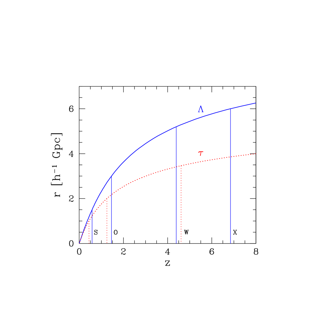
Figure 1.— Comoving look–back distance as a function of redshift for $\Lambda$CDM (solid) and $\tau$CDM (dashed). Vertical lines indicate redshift limits of the spherical (S), octant (O), deep wedge (W) and extended wedge (X) surveys (Table 2).

     

Figure 2.— Maps of the dark matter in slices through the deep octant surveys in (a) $\tau$CDM and (b) $\Lambda$CDM world models. Survey origins are at the vertices (O), and color represents mass density relative to the mean ranging from $0.05$ (black) to 50 (white) on a logarithmic scale. Density is mapped onto a two-dimensional grid using an adaptive (Lagragian) smoothing kernel with scale $2\times 10^{13}\hbox{$\,h^{-1}$}{\rm M}_{\odot}$. For each model, two representations of a $45^{\circ}$ slice extending to $z\!=\!1.25$ are shown. Horizontal maps display structure in the comoving metric while the vertical maps display the same comoving region, reflected about the diagonal, in redshift space. Positions of clusters at the intersection of filaments are evident in redshift space through the radial distortions arising from their internal velocity dispersions (so–called ‘fingers of God’). The inset of the $\tau$CDM image shows the relation between comoving distance $r$ and redshift $z$ over the range mapped by the images. The inset of the $\Lambda$CDM image shows a close-up of the particle distribution around the largest cluster of the $\Lambda$CDM octant surveys, located at $z\!=\!1.04$. Particles colored white lie within a sphere of physical radius $1.5\hbox{$\,h^{-1}$}{\rm\ Mpc}$ that encompasses a mean density 200 times the critical value.

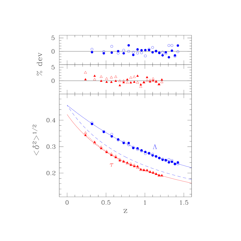
Figure 3.— Redshift evolution of the rms amplitude of density fluctuations $\langle\delta^{2}\rangle^{1/2}$ in top-hat spheres containing, on average, a mass of $2.2\times 10^{15}\hbox{$\,h^{-1}$}{\rm M}_{\odot}$ (1000 particles). Points are octant survey measurements (filled, PO; open, NO) from the $\Lambda$CDM (circles) and $\tau$CDM (triangles) simulations, obtained by randomly sampling twenty radial shells of equal comoving volume and plotted at the volume-weighted redshift of each shell. Solid lines are predictions from linear theory based on the input fluctuation spectra. The upper panel demonstrates agreement with linear theory at the $\!\sim\!1\%$ level, except for the non-linear departure of $\tau$CDM fluctuations at late times. The dashed line in the lower panel shows the evolution that $\Lambda$CDM fluctuations would have if they followed the $\tau$CDM linear growth evolution.

     

Figure 4.— Redshift-space structure in $75,000\hbox{ km s${}^{-1}$}$ wide regions centered at $z\!=\!1.1$ in $\tau$CDM (left) and $\Lambda$CDM (right). The grey-scale shows only overdense material $\delta>0$. The $\Lambda$CDM image includes the most massive cluster in the octant surveys, visible as the long streak at the lower right. The regions shown lie just interior to the vertical edges of the redshift-space maps of Figure 2.

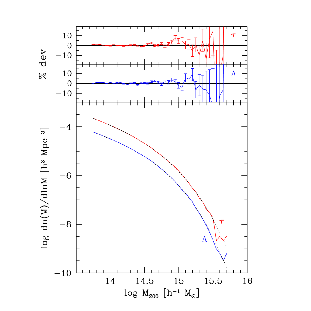
Figure 5.— The lower panel shows critical SO(200) mass functions derived from the $z\!=\!0$ HV cluster catalogs (solid lines) along with fits to the Jenkins’ mass function, equation (10), using parameters listed in Table 4 (dotted lines). Upper panels show the percent deviation in number density between the HV data and the fits. Error bars are based on Poisson statistics in each mass bin.

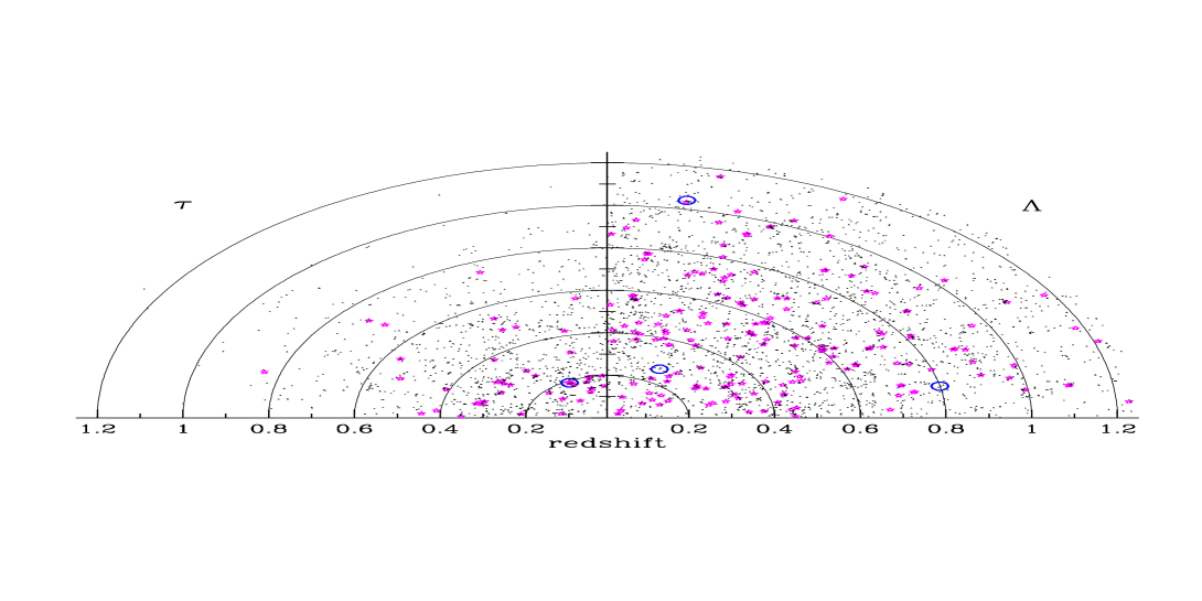
Figure 6.— Maps of clusters in $90^{\circ}\times 3^{\circ}$ slices extending to $z\!=\!1.25$, derived from the octant sky surveys of the $\tau$CDM (left) and $\Lambda$CDM (right) models. Symbols shows clusters of different masses: $hM_{200}/{\rm M}_{\odot}>10^{15}$ (open circles); $\in 10^{14.5}-10^{15}$ (stars) and $\in 10^{14}-10^{14.5}$ (dots). Numbers of clusters in these mass ranges are 1, 50, 1071 ($\tau$CDM) and 3, 185, 2896 ($\Lambda$CDM).

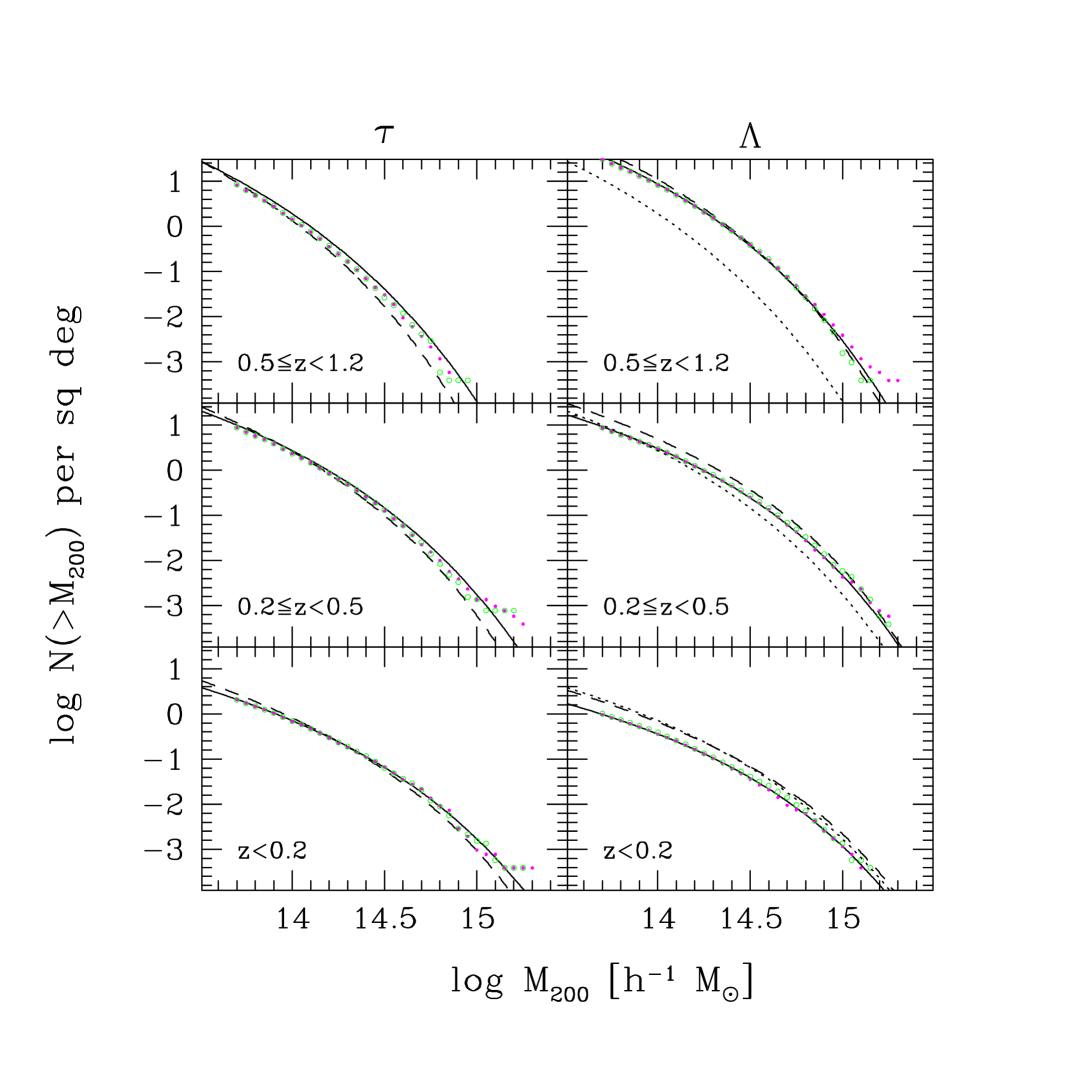
Figure 7.— Cumulative sky counts of clusters as a function of mass for low, intermediate and high redshift intervals (bottom to top) for $\tau$CDM (left) and $\Lambda$CDM (right). Smooth solid lines in each panel give the expectations from integrating the Jenkins mass function, equation (10), over the appropriate volumes. Points show counts from the PO (filled circles) and NO (open) octant surveys. Dashed lines are standard Press–Schechter estimates. In the $\Lambda$CDM panels, dotted lines display the corresponding JMF expectations for the $\tau$CDM cosmology.

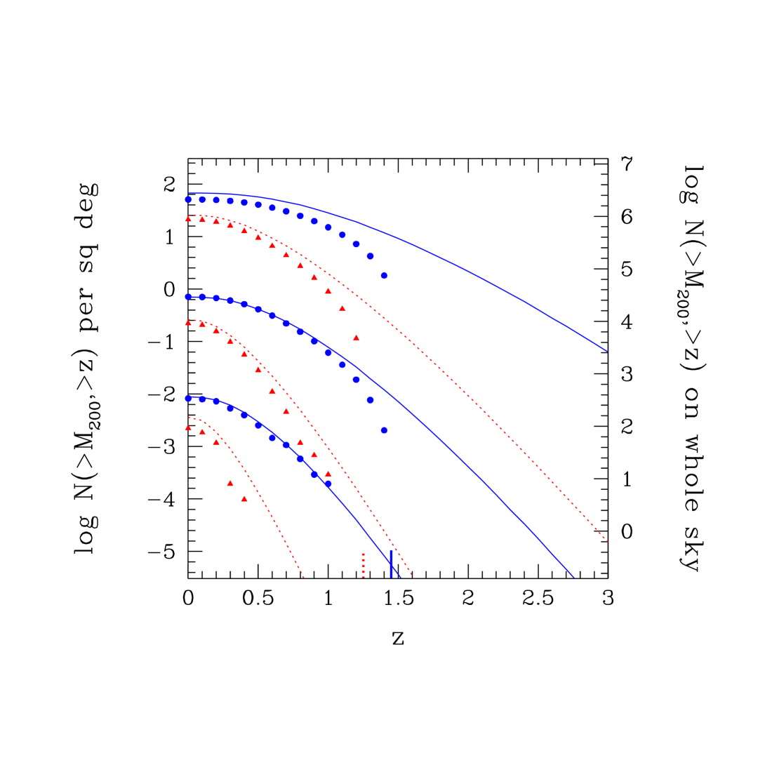
Figure 8.— Sky surface density of clusters lying at redshift $z$ or higher in $\Lambda$CDM (filled circles, solid lines) and $\tau$CDM (filled triangles, dotted lines). Points give numbers derived from the combined octant surveys with masses above $\hbox{$M_{200}$}\!=\!5\times 10^{13}$ (top), $3\times 10^{14}$ (middle) and $10^{15}\hbox{$\,h^{-1}$}{\rm M}_{\odot}$ (bottom). Short vertical lines mark the limiting redshifts of the octant surveys. Lines are expectations at each mass limit derived from integrating the Jenkins mass function.

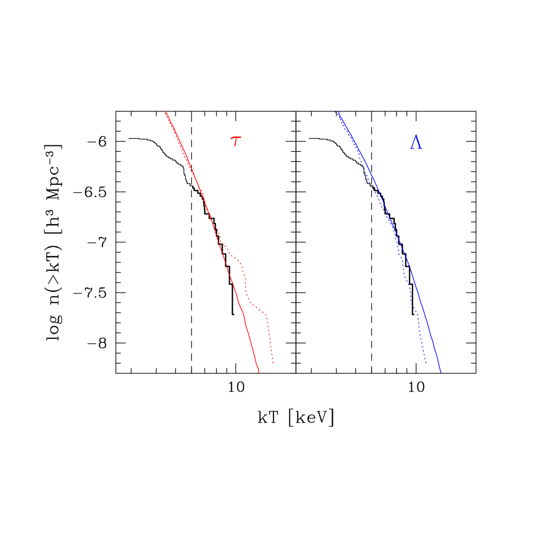
Figure 9.— Thick lines show the local temperature function of Pierpaoli et al. (2001) based largely on data of Markevitch (1998). The HV simulation expectations, using best-fit values $\hbox{$\beta_{\Lambda}$}\!=\!0.92$ and $\hbox{$\beta_{\tau}$}\!=\!1.20$, are shown from the light-cone (dotted) and $z\!=\!0$ snapshot (solid) outputs. The former uses clusters within the combined MS and VS surveys lying in the redshift interval $0.03<z<0.09$. The latter uses the cluster population of the entire computational volume. The vertical dashed line in each panel shows the approximate completeness limit of the observations.

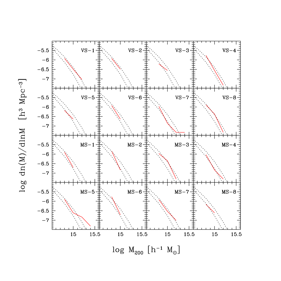
Figure 10.— Differential mass functions within 16 independent $\pi/2$ steradian regions extending to $z\!=\!0.15$, derived from the MS and VS surveys of the $\Lambda$CDM model. Dashed lines show JMF expectations, equation (10), for $\sigma_{8}$ values varied by $\pm 5\%$ about the input value linearly evolved to $z\!=\!0.1$. The volume of the samples is comparable to that of the local observed sample used to constrain $\sigma_{8}$.

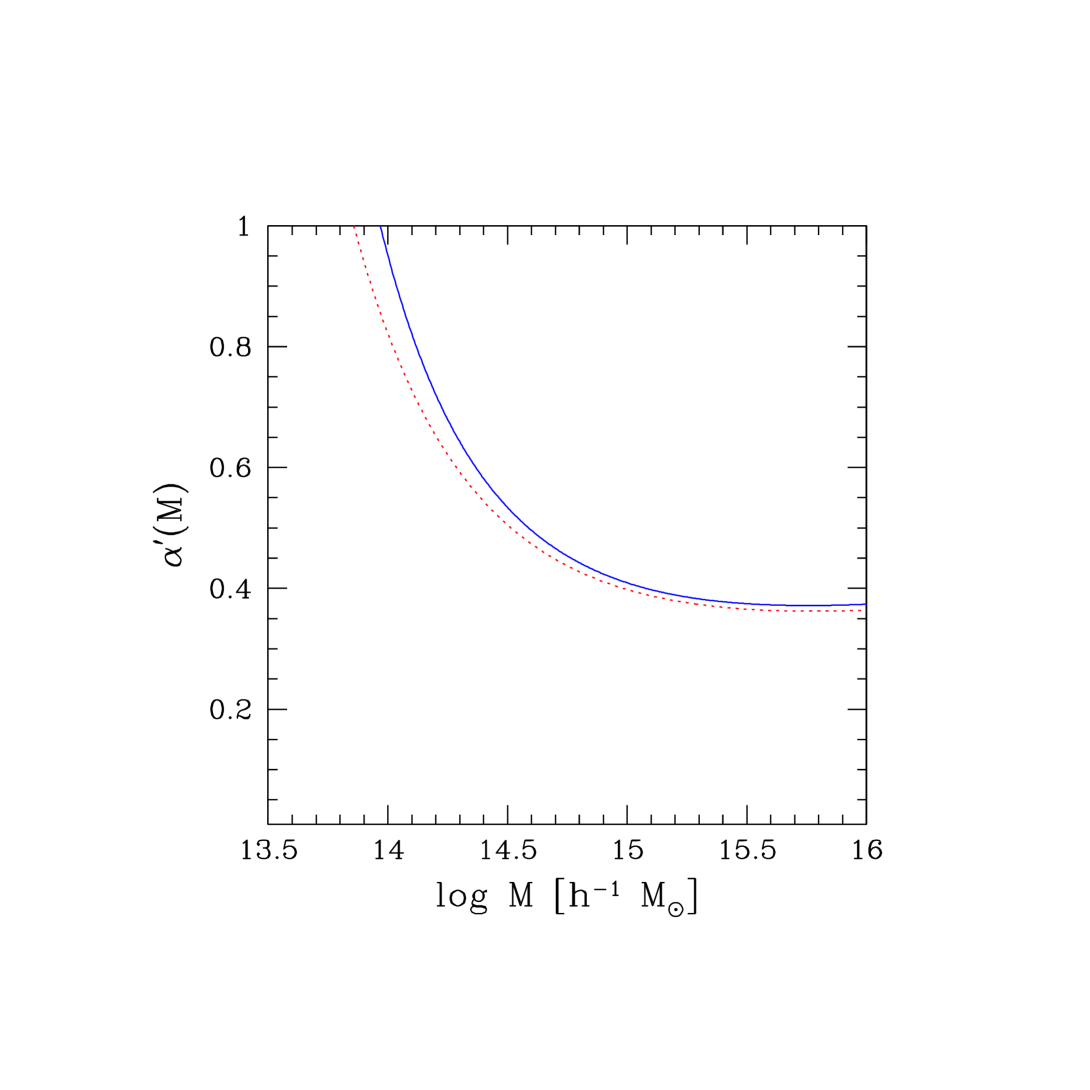
Figure 11.— The sensitivity $\alpha^{\prime}(M)$, equation (14), for the $\Lambda$CDM (solid) and $\tau$CDM (dotted) models.

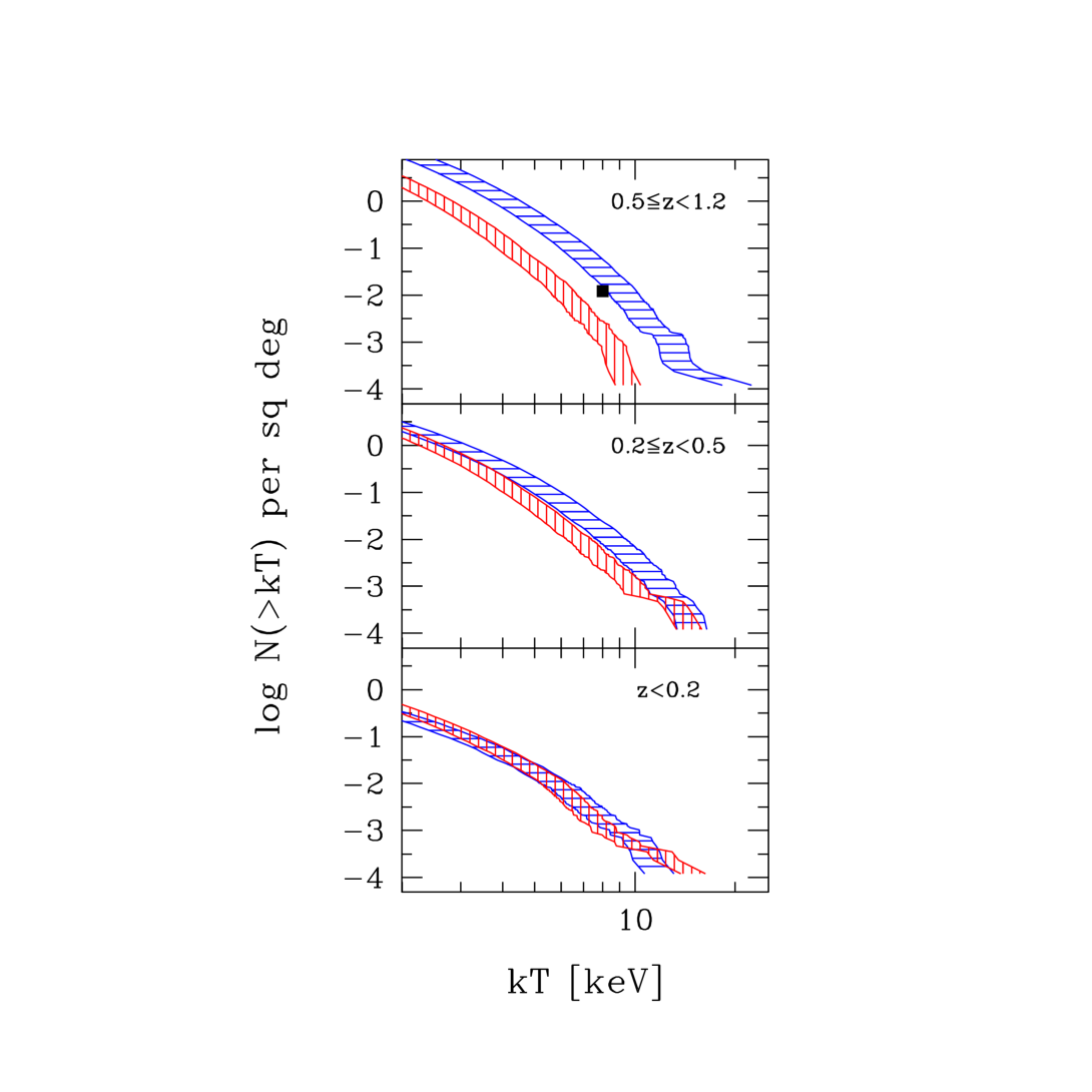
Figure 12.— The range of cumulative sky surface densities of clusters as a function of temperature in three redshift intervals for the $\Lambda$CDM (horizontal hatched) and $\tau$CDM (vertical) cosmologies. The range is determined from the combined octant survey counts by varying $\beta$ within its overall $5$ to $95\%$ confidence range. The solid square denotes the EMSS observational result for clusters hotter than 8 keV at $z>0.5$.

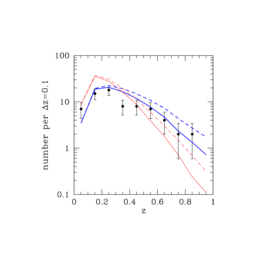
Figure 13.— Points show the redshift distribution of the X–ray flux-limited RDCS survey (Rosati et al. 1998; Borgani et al. 1999b), with Poissonian errors. Solid lines show expectations for a $33$ sq deg survey derived from the combined octant surveys by assuming constant $\beta$ and a non-evolving $L_{X}$–$T$ relation. Dashed lines show plausible confusion effects of core luminosity contamination on the X–ray-selection (see text for details).

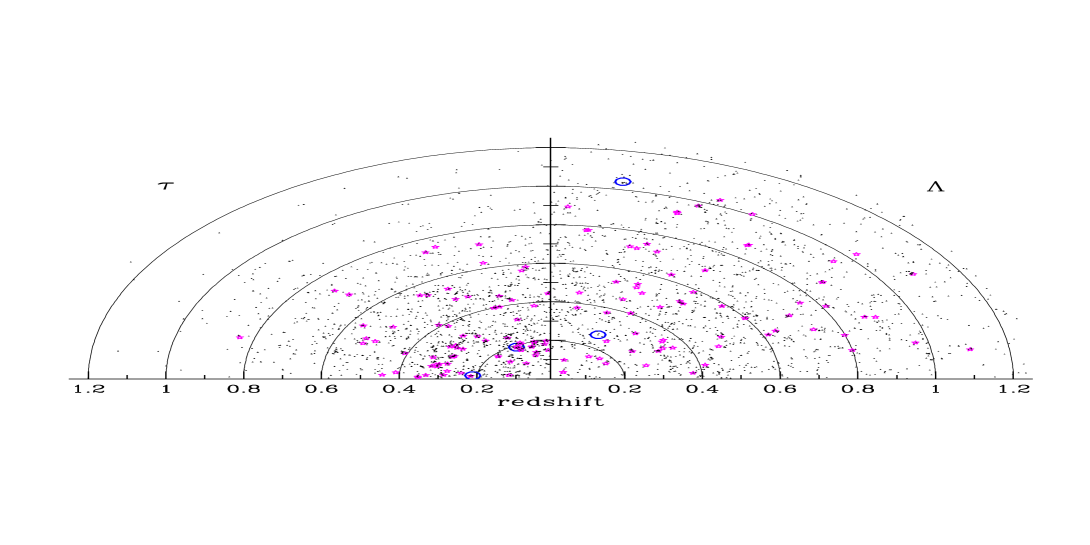
Figure 14.— Clusters expected in the same $90^{\circ}\times 3^{\circ}$ slices shown in Figure 6, but shown here after application of effective biases in $\sigma_{8}$ of $+10\%$ ($\tau$CDM) and $-10\%$ ($\Lambda$CDM).

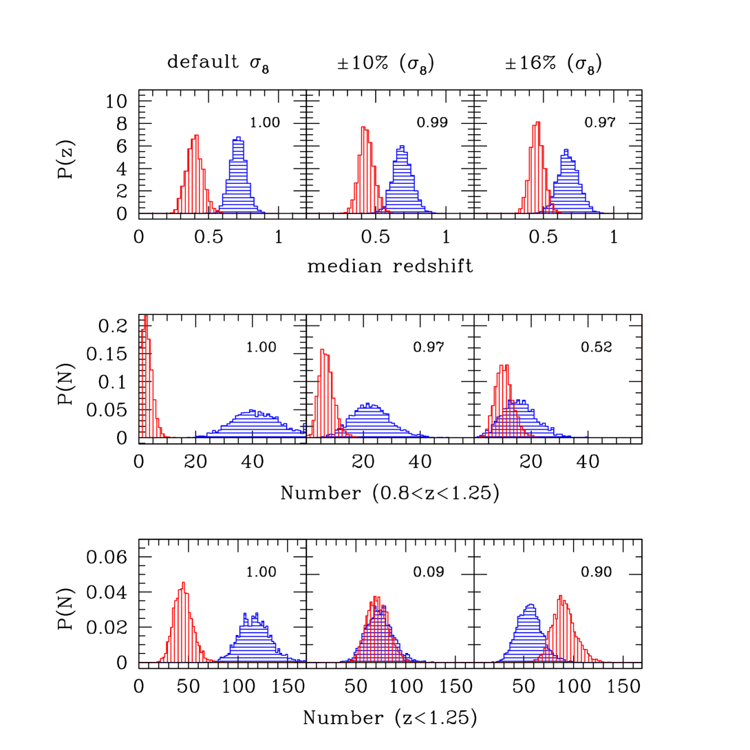
Figure 15.— The influence of varying $\sigma_{8}$ on the population of clusters more massive than $10^{14}\hbox{$\,h^{-1}$}{\rm M}_{\odot}$ expected in 10 sq deg survey fields. Columns (left to right) show probability distributions at the default $\sigma_{8}$ values, $(+/-)10\%$ and $(+/-)16\%$ variation ($+$ for $\tau$CDM/$-$ for $\Lambda$CDM) for the counts at redshifts $z<1.25$ (bottom row), counts in the high redshift interval $0.8<z<1.25$ (middle) and the median cluster redshift (top). Vertical hatched distributions are $\tau$CDM, horizontal are $\Lambda$CDM. Numbers in each panel give the power statistic described in the text. The distributions are generated by sampling 10 sq deg fields around 3000 randomly chosen pointings in the combined octant surveys of each model. Shifts in mass and number, equation (5.2) are used to effectively vary $\sigma_{8}$ in the cluster catalogs.

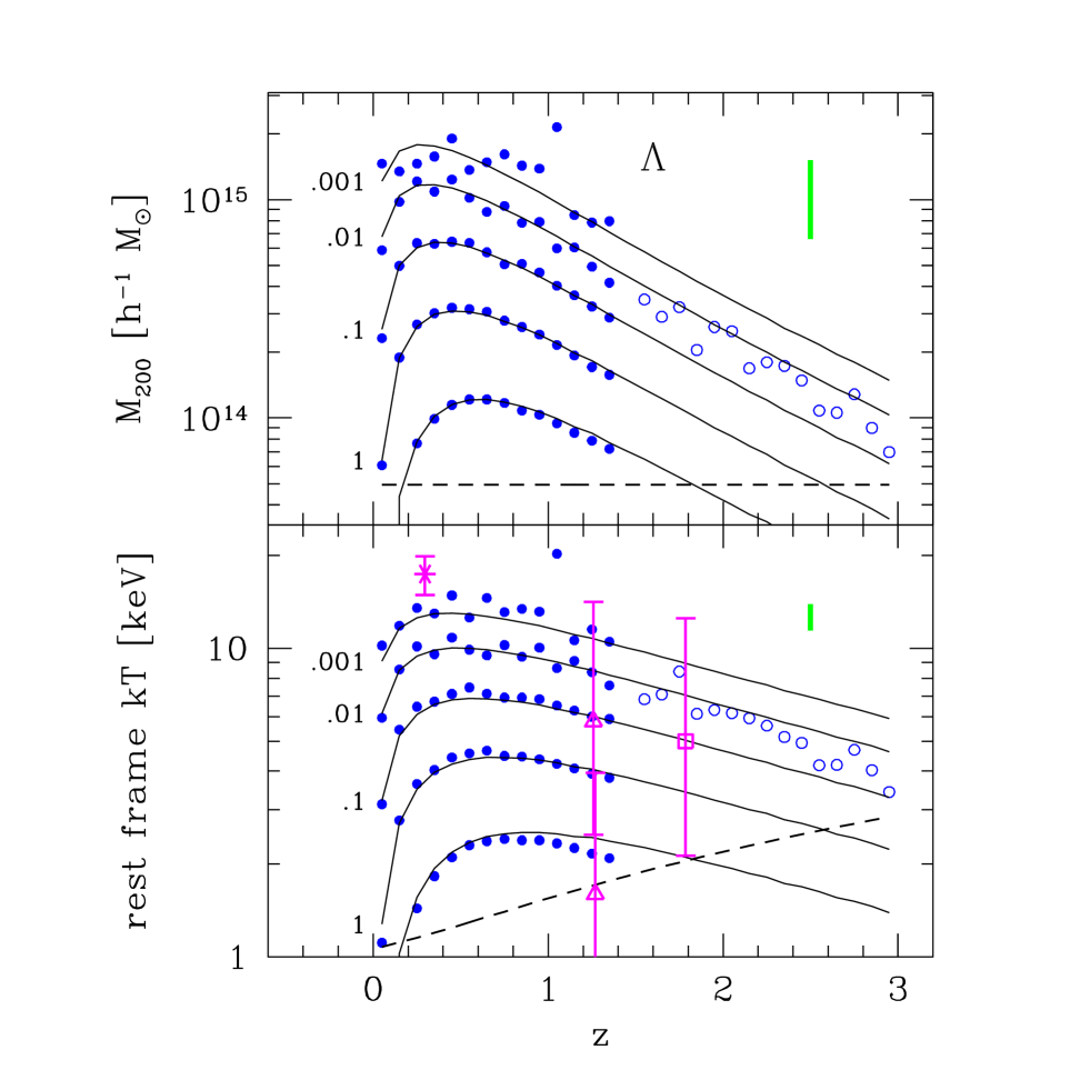
Figure 16.— Sky surface density characteristic mass (upper) and temperature (lower) in the $\Lambda$CDM model. Points from the 10,000 sq deg combined octant surveys (filled circles) and the 1000 square degree extension (open circles) show values above which the cluster sky surface density in the redshift interval $z-0.05$ to $z+0.05$ exceeds values $0.001$, $0.01$, $0.1$, 1 and 10 per sq deg per unit redshift. Clusters at the lowest sky density shown are the most massive or hottest in the particular redshift interval within the combined octants. Note the exceptional ‘monster’ cluster at $z\!=\!1.04$. Solid lines are JMF expectations described in the text. Vertical bars in each panel denote the $90\%$ confidence uncertainty range in the absolute calibration of mass and temperature scales. Open triangles and squares plot extremes of the known X–ray cluster population: RX J0849+4452 at $z\!=\!1.26$ and RX J0848+4453 at $z\!=\!1.27$ (Stanford et al. 2000, triangles); 3C294 at $z\!=\!1.786$ (Fabian et al. 2001, square) and 1E 0657-56 at $z\!=\!0.296$ (Tucker et al. 2001, asterisk). Dashed lines show a mass limit of 22 simulation particles (upper panel) and the virial temperature at that mass (lower).

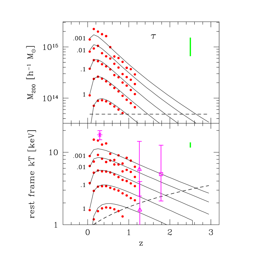
Figure 17.— Same as Figure 16, but for the $\tau$CDM model.

Appendix A A. Cluster Finding Details and Completeness Checks

The cluster finding algorithm that produced the catalogs in this paper begins by generating a density estimate for each particle using the distance to its eighth nearest neighbor (Casertano & Hut 1985), equivalent to Lagrangian filtering on a mass scale $2\times 10^{13}\hbox{$\,h^{-1}$}{\rm M}_{\odot}$. Sorting density values in decreasing order provides a list of potential sites for cluster centers. The list is pruned by eliminating particles whose densities lie below the threshold $\hbox{$\Delta$}\hbox{$\rho_{c}$}(z)$. Beginning with the first member of the sorted list, a sphere of radius $r_{\Delta}$ enclosing mass $M_{\Delta}$ is defined about that particle so that the enclosed density $\rho\!\equiv\!3\hbox{$M_{\Delta}$}/4\pi{\hbox{$r_{\Delta}$}}^{3}\!=\!\hbox{$\Delta$}\rho_{c}(z)$. Particles lying within this sphere are recorded as members of this group and are removed from the list of potential cluster centers. The process is repeated sequentially, centering on the next available particle in the list ordered by decreasing density, until the list is exhausted. Particles may belong to more than one group, but the center of a given group never lies within the spherical boundary of another group.

In analyzing SO(180) and mean SO(324) populations of the $\tau$CDM and $\Lambda$CDM models, respectively, J01 noted a problem of incompleteness in the SO cluster finding algorithm at particle counts $\mathrel{\hbox to0.0pt{\lower 3.0pt\hbox{$\mathchar 536\relax$}\hss}\raise 2.0pt\hbox{$\mathchar 316\relax$}}100$. Resolution tests in J01 indicated that space densities of groups comprised of 20 particles could be underestimated by $\!\sim\!30\%$. We employ here an independent SO algorithm with improved completeness properties at small numbers of particles. Figure 1 compares the SO(180) and mean SO(324) abundance functions (for $\tau$CDM and $\Lambda$CDM, respectively) at $z\!=\!0$ based on the new algorithm to the fits published in Appendix B of J01.

In the figure, the thick solid line show J01 functional fits while the thin solid and dotted lines show discrete mass functions derived with the algorithm employed here. The dot-dashed line is the discrete $\tau$CDM mass function derived by J01 using the previous SO algorithm. The top panel shows the percent deviation between the discrete sample measurements and the fit expectations.

For the $\tau$CDM case, both the old and new algorithms compare well against each other and against the fit above $\sim\!10^{15}\hbox{$\,h^{-1}$}{\rm M}_{\odot}$. At lower masses, the J01 algorithm displays an increasing underestimate in number density with respect to the fit, approaching a $30\%$ underestimate at the mass limit $5\times 10^{13}\hbox{$\,h^{-1}$}{\rm M}_{\odot}$ used in this work. The new SO algorithm (dotted) displays a similar qualitative trend, but the underestimate is reduced to $\mathrel{\hbox to0.0pt{\lower 3.0pt\hbox{$\mathchar 536\relax$}\hss}\raise 2.0pt\hbox{$\mathchar 316\relax$}}10\%$ in amplitude. A similar trend is seen for the new algorithm in the $\Lambda$CDM case where the number density lies $\sim\!12\%$ lower than the J01 fit expectations. This analysis indicates that the amplitude $A$ derived from fitting the space density to the Jenkins form, to equation (10), may be biased low by $\sim\!10\%$ at masses below $\sim\!10^{15}\hbox{$\,h^{-1}$}{\rm M}_{\odot}$.

A further check of resolution effects is made by directly comparing the HV mass function to one derived from smaller volumes with improved mass resolution. We do this for SO(200) clusters in the $\Lambda$CDM model at $z\!=\!0$, using data from the $256^{3}$ particle simulation of a $239.5\hbox{$\,h^{-1}$}{\rm\ Mpc}$ region from Jenkins et al. (1998). The new SO(200) algorithm is used to identify clusters in the same manner as done in the HV simulation. The cosmological parameters for the models are the same, except for a slight difference in the power spectrum used to generate the initial conditions, whereas the particle mass in the $256^{3}$ particle simulation is a factor 32 times smaller than that used in the HV computations.

Figure 2 shows the cumulative number of clusters found in the $256^{3}$ particle simulation (dotted line) along with the number expected based on the $z\!=\!0$ HV population (solid). Vertical bars on the HV results show the range in number derived from dividing the HV volume into 1728 independent cubes of side $250\hbox{$\,h^{-1}$}{\rm\ Mpc}$ and rescaling the counts in each cube to a $(239.5\hbox{$\,h^{-1}$}{\rm\ Mpc})^{3}$ volume. The inset shows the correlation between counts above $5\times 10^{13}$ and $3\times 10^{14}\hbox{$\,h^{-1}$}{\rm M}_{\odot}$ within the subvolumes. The small–volume simulation result is inconsistent with the HV distribution; the count distribution shows agreement at the $98\%$ level at $3\times 10^{14}\hbox{$\,h^{-1}$}{\rm M}_{\odot}$ but the $5\times 10^{13}$ count is $\sim\!0.5\%$ higher than the maximum of the HV distribution and $\!\sim\!20\%$ above the mean.

These findings, along with the slight discrepancy in predicted versus measured counts in the $\tau$CDM octant surveys (Figure 7) lead to a conservative estimate of the systematic theoretical uncertainty in the number density of clusters above $10^{14}\hbox{$\,h^{-1}$}{\rm M}_{\odot}$ to be $20\%$. Future studies, in particular those which cross-calibrate results for a particular cosmology modeled by different simulation teams, are needed to better assess the overall accuracy of this model of the mass function.

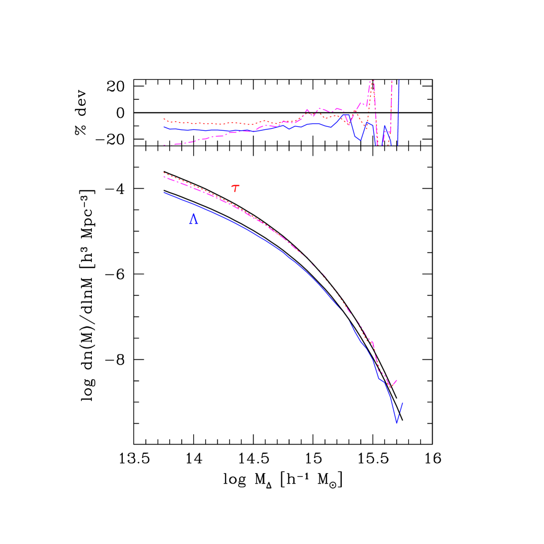
Figure 1.— Differential SO mass functions at $z\!=\!0$ are compared to the fits published in J01. In the lower panel, thick lines are the J01 expectations (from their Appendix B) for $\tau$CDM at $\hbox{$\Delta$}\!=\!180$ (upper curve) and $\Lambda$CDM at mean $\hbox{$\Delta$}\!=\!324$ (critical $\hbox{$\Delta$}\!=\!97.2$, lower curve). The $\Lambda$CDM simulation data are shown by the slightly jagged solid curve. Two simulation results are shown for $\tau$CDM— the dot-dashed line reflects the SO algorithm used by J01 and the dotted line shows results of the algorithm used in this work. The upper panel displays the percent deviation in number density between the HV simulation data and the J01 model fits.

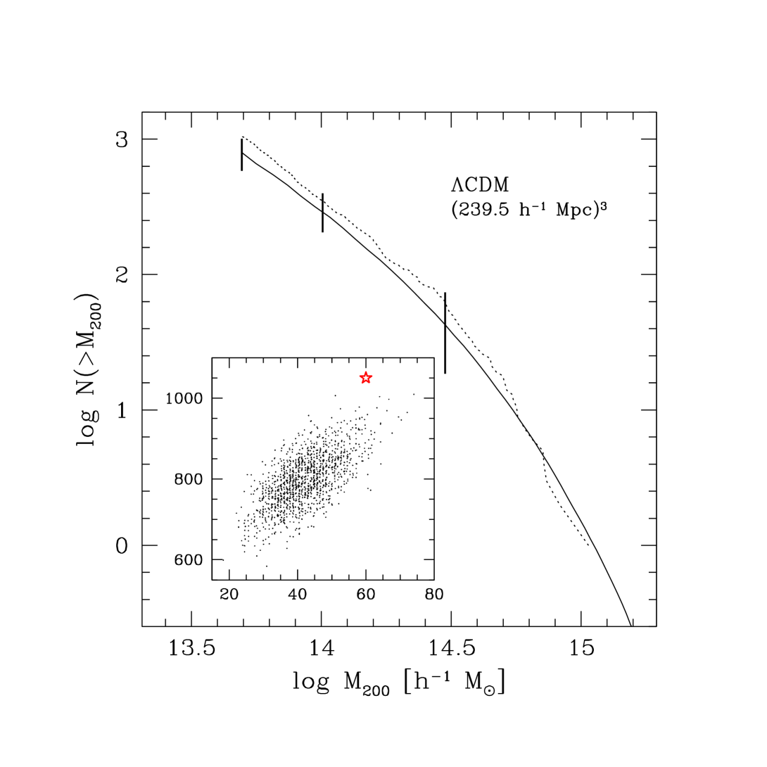
Figure 2.— The cumulative number of clusters within the volume indicated, scaled from the full $z\!=\!0$ HV simulation (solid line) and from a single realization of a $(239.5\hbox{$\,h^{-1}$}{\rm\ Mpc})^{3}$ volume (Jenkins et al. 1998; dotted line) for the $\Lambda$CDM cosmology. Vertical lines show the entire range of counts above masses $5\times 10^{13}$, $10^{14}$ and $3\times 10^{14}\hbox{$\,h^{-1}$}{\rm M}_{\odot}$ derived from subsampling 1728 cubic sub-volumes of side $250\hbox{$\,h^{-1}$}{\rm\ Mpc}$ within the HV realization and scaling to $239.5\hbox{$\,h^{-1}$}{\rm\ Mpc}$. The inset plots the correlation of counts above $3\times 10^{14}$ ($x$-axis) and $5\times 10^{13}$ ($y$-axis) derived from the sub-volumes. The star indicates the Jenkins et al. (1998) values.

Appendix B B. Mass scale renormalization

The mass scale of clusters at fixed space density is uncertain, both theoretically and empirically, for reasons discussed in the opening section. The lack of a uniquely defined scale motivates a model that would transform the JMF fit parameters derived in §3.3 to values appropriate for a redefined mass scale. As an example, we develop here a model to estimate the SO mass function fit parameters for threshold values $\Delta\neq 200$. The method is similar to that used in §5.2 to effectively vary $\sigma_{8}$ within the discrete cluster samples.

We have chosen a convention in which a spherical density threshold $\Delta\!=\!200$ defines cluster masses $M$. A choice $\Delta\neq 200$ would lead to a new mass $M^{\prime}$ for each cluster related to the original by some factor

$$M^{\prime}\ =\ M\,e^{\mu}.$$ (B1)

The space density of a set of disjoint clusters is fixed, implying

$$n(M^{\prime})\,\hbox{\rm d$\,$ln }\!M^{\prime}\ =\ n(M)\,\hbox{\rm d$\,$ln }\!M.$$ (B2)

This condition, with equation (B1), when used with the space density, equation (10), leads to a relation between JMF parameters

$$A^{\prime}\ =\ A\,e^{\mu}$$

$$B^{\prime} \ =\ B-\alpha_{\rm eff}(M)\,\mu$$ (B3)

to first order in $\mu$.

The factor $\mu$ can be calculated from an assumed mass profile. We use the form introduced by Navarro et al. (1996; hereafter NFW),

$$M(x)\ =\ \frac{800\pi}{3}\,\hbox{$\rho_{c}$}\,\hbox{$r_{200}$}^{3}\biggl{[}\frac{\ln(1+cx)-cx/(1+cx)}{\ln(1+c)-c/(1+c)}\biggr{]}$$ (B4)

where $x\!=\!r/\hbox{$r_{200}$}$ is a scaled radius and $c$ is a concentration parameter. N–body simulations suggest $c\!\simeq\!5$ at masses near $10^{15}\hbox{$\,h^{-1}$}{\rm\ Mpc}$ for the cosmologies studied here (NFW, Frenk et al. 1999; Jing 2000; Bullock et al. 2001).

Figure 1 shows the results of applying equation (B) to critical contrasts $\Delta\!=\!97.2$ and $500$ for the $\Lambda$CDM model, assuming $c\!=\!5$. The logarithmic shifts in mass scale are $\mu\!=\!0.093$ and $-0.141$, respectively. The agreement between the predicted and measured values is quite good. At $\Delta\!=\!97.2$ (equivalent to the mean contrast of $324$ used by J01), the bin-averaged mean fractional error and dispersion (for bins with $10\%$ or less Poisson uncertainty) are only $4.1\%$ and $3.8\%$. At $\Delta\!=\!500$, the mean is $-14.5\%$ and dispersion $4.9\%$.

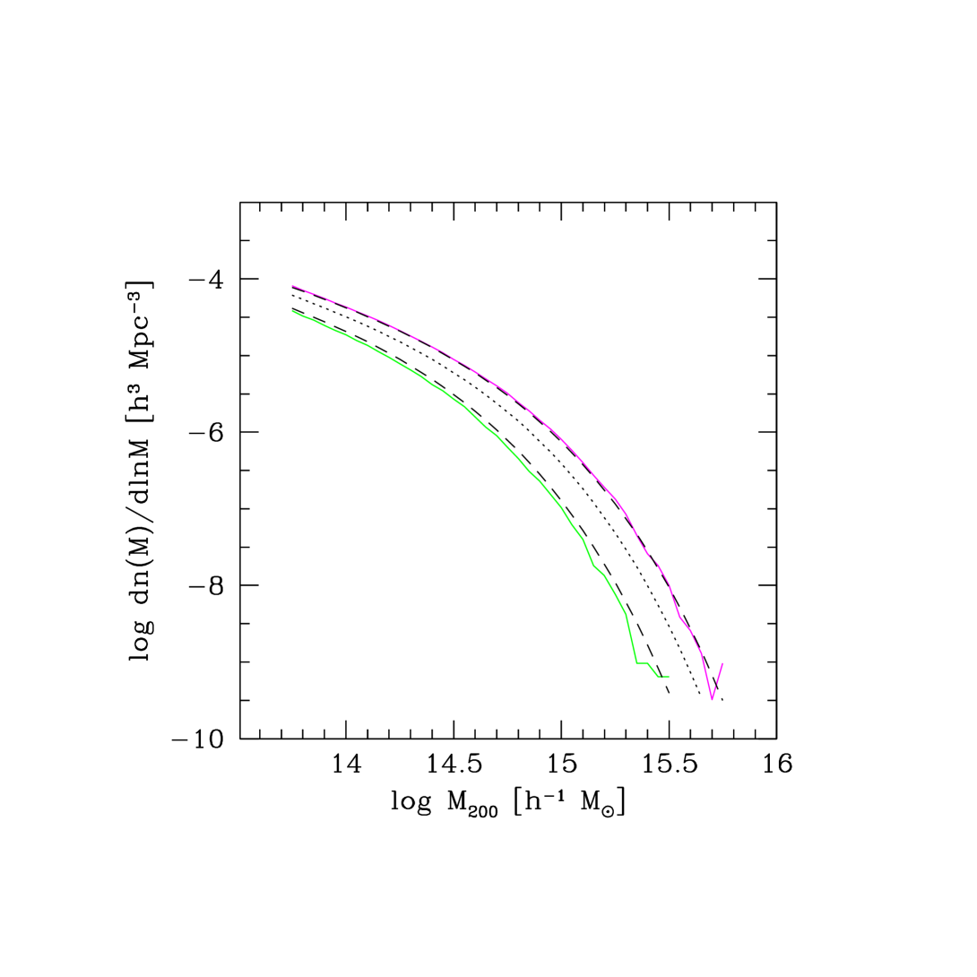
Figure 1.— The critical SO(500) and SO(97.2) mass functions (lower and upper, respectively) at $z\!=\!0$ for $\Lambda$CDM. Solid lines are measured from the HV simulation while dashed lines are predictions based on rescaling the SO(200) JMF fit (dotted line), assuming an NFW profile with concentration parameter $c\!=\!5$.

Appendix C Cluster catalogs

The SO(200) cluster catalogs derived from the sky survey and $z\!=\!0$ snapshot outputs of the simulations are included here as electronic tables. In the print edition, Tables 6 through 17 provide a truncated listing of the ten most massive clusters for each survey. Electronic versions list all clusters resolved above a mass limit of 22 particles ($5\times 10^{13}\hbox{$\,h^{-1}$}{\rm M}_{\odot}$), counts of which are listed in Table 5. Tables 6 through 11 are $\Lambda$CDM simulation catalogs from the $z\!=\!0$ snapshot, the combined PO and XW sky surveys, and the NO, VS, MS and DW sky surveys, respectively. Tables 12 through 17 provide the same for $\tau$CDM, with the exception that there is no extended wedge associated with the PO survey of this model (see Table 2).

Column entries give the mass $M_{200}$ (in $10^{15}\hbox{$\,h^{-1}$}{\rm M}_{\odot}$), redshift (for sky survey data) derived from Hubble flow and the radial peculiar velocity, one-dimensional velocity dispersion $\sigma_{v}$ determined from a three-dimensional average (in km s^-1), position in comoving coordinates (in $\,h^{-1}$ Gpc), and peculiar velocity (in km s^-1). The position is defined as the location of the particle having the smallest distance to its eighth neighboring particle (see Appendix A), and the peculiar velocity is defined by the mass-weighted mean within $r_{200}$.

Table 6Clusters in the $\Lambda$CDM $z=0$ snapshot survey.

$M_{200}$	$\sigma$	$x$	$y$	$z$	$v_{x}$	$v_{y}$	$v_{z}$
$10^{15}\hbox{$\,h^{-1}$}{\rm M}_{\odot}$	km s-1	$\hbox{$\,h^{-1}$}{\rm\ Gpc}$	$\hbox{$\,h^{-1}$}{\rm\ Gpc}$	$\hbox{$\,h^{-1}$}{\rm\ Gpc}$	km s-1	km s-1	km s-1
4.7745	1795	2.27792	0.44894	0.54195	-90	153	-6
4.7475	1866	2.03410	0.91683	0.44397	269	46	727
4.2840	1781	1.74103	2.84553	1.40265	87	-52	-154
3.9645	1632	0.96734	0.65102	2.32061	63	312	-282
3.8227	1891	1.75213	0.72151	1.80426	380	-90	-279
3.4920	1665	1.50312	1.77336	2.19206	-26	1	-17
3.3772	1531	1.21292	2.12486	0.27272	-434	-228	-821
3.3592	1583	2.50579	2.18682	0.31021	-183	588	174
3.3187	1519	2.07928	2.97238	1.91753	-532	-531	-156
3.2602	1566	0.38232	1.70524	0.62298	-228	257	98

Table 7Clusters in the $\Lambda$CDM PO+XW sky survey

$M_{200}$	redshift	$\sigma$	$x$	$y$	$z$	$v_{x}$	$v_{y}$	$v_{z}$
$10^{15}\hbox{$\,h^{-1}$}{\rm M}_{\odot}$		km s-1	$\hbox{$\,h^{-1}$}{\rm\ Gpc}$	$\hbox{$\,h^{-1}$}{\rm\ Gpc}$	$\hbox{$\,h^{-1}$}{\rm\ Gpc}$	km s-1	km s-1	km s-1
2.1465	1.04210	1740	2.27834	0.44795	0.54248	229	319	-99
1.9035	0.49167	1490	0.48208	1.20790	0.20341	287	-806	-725
1.8337	0.48731	1473	1.25433	0.30248	0.12419	300	-692	13
1.6245	0.48492	1440	1.25607	0.30110	0.12310	-520	45	327
1.6132	0.74772	1389	0.38256	1.70412	0.62232	171	-58	192
1.5052	0.48217	1339	1.00142	0.47311	0.64768	-177	670	268
1.4850	0.63925	1309	1.21259	0.74437	0.79747	-4	-6	406
1.4265	0.33432	1338	0.15125	0.88516	0.24984	-533	-287	-210
1.3927	0.26386	1273	0.62241	0.37143	0.16475	283	50	-310
1.3860	0.95680	1403	1.28228	0.28511	1.81830	-107	-259	41

Table 8Clusters in the $\Lambda$CDM NO sky survey

$M_{200}$	redshift	$\sigma$	$x$	$y$	$z$	$v_{x}$	$v_{y}$	$v_{z}$
$10^{15}\hbox{$\,h^{-1}$}{\rm M}_{\odot}$		km s-1	$\hbox{$\,h^{-1}$}{\rm\ Gpc}$	$\hbox{$\,h^{-1}$}{\rm\ Gpc}$	$\hbox{$\,h^{-1}$}{\rm\ Gpc}$	km s-1	km s-1	km s-1
1.8720	0.47097	1357	0.78598	0.89484	0.40376	-13	365	-193
1.6762	0.45872	1332	0.25973	1.14905	0.34105	-128	508	-150
1.5750	0.39013	1393	0.50888	0.89409	0.29059	-106	-92	-379
1.4985	0.36176	1308	0.54647	0.73774	0.40355	-467	-203	-432
1.4625	0.09295	1230	0.11250	0.20762	0.13595	114	63	68
1.4602	0.21513	1254	0.13535	0.45678	0.38800	-624	336	-46
1.4422	0.23629	1209	0.21785	0.32614	0.54597	41	299	-195
1.4310	0.84337	1304	1.25924	0.15777	1.59600	-158	-124	27
1.3612	0.25340	1225	0.35217	0.57399	0.23736	-38	458	-21
1.3567	0.24869	1277	0.68191	0.11578	0.14755	46	-19	-1027

Table 9Clusters in the $\Lambda$CDM VS sky survey

$M_{200}$	redshift	$\sigma$	$x$	$y$	$z$	$v_{x}$	$v_{y}$	$v_{z}$
$10^{15}\hbox{$\,h^{-1}$}{\rm M}_{\odot}$		km s-1	$\hbox{$\,h^{-1}$}{\rm\ Gpc}$	$\hbox{$\,h^{-1}$}{\rm\ Gpc}$	$\hbox{$\,h^{-1}$}{\rm\ Gpc}$	km s-1	km s-1	km s-1
3.7710	0.36705	1849	0.77855	1.94855	2.04204	-179	109	-38
2.3985	0.12317	1427	1.66806	1.18289	1.50177	-100	-204	-269
2.1847	0.31494	1513	1.16682	1.78942	0.74591	-276	55	-309
2.1352	0.22786	1510	1.83355	0.95563	1.60533	228	-71	352
2.0407	0.25998	1427	1.69566	2.12671	1.17188	-529	84	-410
2.0385	0.27780	1536	1.14664	2.02703	1.04228	-73	94	220
1.9957	0.21552	1393	1.20062	1.88904	1.87100	60	546	-365
1.9282	0.17104	1473	1.83406	1.48791	1.14040	367	-434	-99
1.9260	0.38687	1515	1.99907	1.19847	2.37855	294	-141	207
1.9237	0.21232	1425	1.62686	0.92821	1.34563	203	-10	-516

Table 10Clusters in the $\Lambda$CDM MS sky survey

$M_{200}$	redshift	$\sigma$	$x$	$y$	$z$	$v_{x}$	$v_{y}$	$v_{z}$
$10^{15}\hbox{$\,h^{-1}$}{\rm M}_{\odot}$		km s-1	$\hbox{$\,h^{-1}$}{\rm\ Gpc}$	$\hbox{$\,h^{-1}$}{\rm\ Gpc}$	$\hbox{$\,h^{-1}$}{\rm\ Gpc}$	km s-1	km s-1	km s-1
3.0622	0.12208	1765	1.61387	1.63047	1.81743	-135	-43	-404
2.9452	0.20045	1583	1.13968	1.94410	1.59070	37	-315	-414
2.7225	0.21132	1724	1.77946	1.14258	1.88827	41	-144	941
2.6640	0.26329	1622	1.50191	1.77218	2.19369	434	317	-245
2.3692	0.39004	1536	1.21250	0.74412	0.79839	-210	0	684
2.2320	0.53759	1482	1.20256	2.12932	0.26569	636	-375	138
2.1690	0.48039	1534	1.28226	0.28481	1.81857	55	-597	114
2.0925	0.54800	1465	0.38300	1.70434	0.62229	-215	29	239
2.0272	0.47799	1414	1.16678	1.69964	0.28919	308	159	-474
1.9147	0.41372	1393	0.49259	1.31877	1.03747	86	548	-522

Table 11Clusters in the $\Lambda$CDM DW sky survey

$M_{200}$	redshift	$\sigma$	$x$	$y$	$z$	$v_{x}$	$v_{y}$	$v_{z}$
$10^{15}\hbox{$\,h^{-1}$}{\rm M}_{\odot}$		km s-1	$\hbox{$\,h^{-1}$}{\rm\ Gpc}$	$\hbox{$\,h^{-1}$}{\rm\ Gpc}$	$\hbox{$\,h^{-1}$}{\rm\ Gpc}$	km s-1	km s-1	km s-1
1.2667	0.35165	1194	0.52955	0.51554	0.62439	236	159	160
0.7425	0.63063	1020	0.89636	1.04111	0.84907	58	-57	21
0.7335	0.54100	1078	0.83017	0.88976	0.74354	-346	-269	-328
0.6952	0.86474	1077	1.26522	1.12729	1.20595	-417	-122	217
0.6795	0.23262	883	0.42833	0.36816	0.34631	184	-40	-201
0.6277	0.49817	968	0.79520	0.73876	0.75309	24	340	-103
0.6210	0.61920	1075	0.87578	0.91529	0.96280	-130	-498	540
0.5872	0.16708	833	0.29741	0.28511	0.25289	406	-169	-255
0.5557	0.24148	766	0.37255	0.44021	0.38042	331	-714	-279
0.5512	0.52327	998	0.76163	0.87778	0.75294	-389	-179	-160

Table 12Clusters in the $\tau$CDM $z=0$ snapshot survey.

$M_{200}$	$\sigma$	$x$	$y$	$z$	$v_{x}$	$v_{y}$	$v_{z}$
$10^{15}\hbox{$\,h^{-1}$}{\rm M}_{\odot}$	km s-1	$\hbox{$\,h^{-1}$}{\rm\ Gpc}$	$\hbox{$\,h^{-1}$}{\rm\ Gpc}$	$\hbox{$\,h^{-1}$}{\rm\ Gpc}$	km s-1	km s-1	km s-1
4.8840	1912	1.60532	0.11171	1.05673	-273	241	-141
4.8707	1946	1.76731	0.09581	0.98359	206	229	-728
4.7597	1907	0.46288	1.83931	0.73075	402	598	-359
4.3290	1787	1.06007	1.25750	0.15836	195	-102	160
4.3246	1816	0.62941	0.32143	0.59557	-120	462	-43
4.1270	1655	0.18549	1.04133	1.38113	125	-584	-549
4.0448	1820	1.40794	0.55788	0.85002	-596	282	-236
3.8473	1734	0.24495	0.63610	0.51995	169	473	235
3.5209	1688	1.59185	0.02998	1.51849	-21	-1044	-78
3.5187	1569	0.54769	0.03614	1.24131	-125	524	-62

Table 13Clusters in the $\tau$CDM PO sky survey

$M_{200}$	redshift	$\sigma$	$x$	$y$	$z$	$v_{x}$	$v_{y}$	$v_{z}$
$10^{15}\hbox{$\,h^{-1}$}{\rm M}_{\odot}$		km s-1	$\hbox{$\,h^{-1}$}{\rm\ Gpc}$	$\hbox{$\,h^{-1}$}{\rm\ Gpc}$	$\hbox{$\,h^{-1}$}{\rm\ Gpc}$	km s-1	km s-1	km s-1
2.2333	0.15351	1635	0.02751	0.34796	0.21763	-155	234	84
1.9869	0.20570	1568	0.10704	0.52032	0.07637	-219	-55	-49
1.7671	0.39740	1512	0.62955	0.31885	0.59612	-123	640	-105
1.4208	0.26994	1345	0.18684	0.32731	0.55685	934	-132	219
1.3942	0.01660	1259	0.02224	0.05106	0.01156	-742	-559	77
1.2920	0.29180	1311	0.09007	0.52090	0.49083	-153	-70	39
1.2898	0.08068	1246	0.21347	0.08099	0.01491	122	-443	-133
1.2521	0.27828	1341	0.58237	0.37616	0.02971	-206	150	35
1.1500	0.25740	1307	0.43210	0.35366	0.33809	-507	-135	33
1.0811	0.19157	1201	0.42661	0.26000	0.09128	-478	-105	-160

Table 14Clusters in the $\tau$CDM NO sky survey

$M_{200}$	redshift	$\sigma$	$x$	$y$	$z$	$v_{x}$	$v_{y}$	$v_{z}$
$10^{15}\hbox{$\,h^{-1}$}{\rm M}_{\odot}$		km s-1	$\hbox{$\,h^{-1}$}{\rm\ Gpc}$	$\hbox{$\,h^{-1}$}{\rm\ Gpc}$	$\hbox{$\,h^{-1}$}{\rm\ Gpc}$	km s-1	km s-1	km s-1
1.8781	0.16574	1489	0.08750	0.34930	0.25921	532	-14	-310
1.6650	0.23534	1613	0.17937	0.04762	0.57891	-102	-429	-661
1.6228	0.40003	1540	0.64304	0.36559	0.55891	-6	475	93
1.5873	0.23482	1433	0.19753	0.03359	0.57222	-426	-150	-519
1.4119	0.13676	1456	0.15879	0.33140	0.02784	70	401	403
1.2388	0.08092	1148	0.13108	0.17990	0.05517	-93	166	-475
1.1566	0.14827	1301	0.23406	0.24841	0.20322	599	505	-569
1.1433	0.14885	1309	0.15585	0.14787	0.33972	36	-297	142
1.1255	0.13588	1194	0.25388	0.00900	0.26156	275	118	572
1.0922	0.05791	1091	0.03287	0.13919	0.07741	23	353	197

Table 15Clusters in the $\tau$CDM VS sky survey

$M_{200}$	redshift	$\sigma$	$x$	$y$	$z$	$v_{x}$	$v_{y}$	$v_{z}$
$10^{15}\hbox{$\,h^{-1}$}{\rm M}_{\odot}$		km s-1	$\hbox{$\,h^{-1}$}{\rm\ Gpc}$	$\hbox{$\,h^{-1}$}{\rm\ Gpc}$	$\hbox{$\,h^{-1}$}{\rm\ Gpc}$	km s-1	km s-1	km s-1
2.5530	0.08805	1595	1.23821	1.06196	0.96259	-18	-331	78
2.5108	0.15568	1622	1.41088	0.90971	0.98357	-261	-24	-177
2.2333	0.15351	1635	1.02751	1.34795	1.21762	-155	234	84
1.9869	0.20570	1568	1.10704	1.52032	1.07637	-218	-55	-49
1.9358	0.17072	1389	0.96303	1.00973	0.54585	-48	394	126
1.8937	0.16180	1570	0.57437	0.89833	1.00483	410	211	-184
1.8781	0.16574	1489	0.91249	0.65070	0.74078	-532	14	311
1.7671	0.39740	1513	1.62955	1.31885	1.59612	-120	638	-106
1.7560	0.37118	1547	1.46201	0.83718	1.73270	127	852	-638
1.7405	0.24550	1491	0.92007	1.16642	1.59436	-310	137	81

Table 16Clusters in the $\tau$CDM MS sky survey

$M_{200}$	redshift	$\sigma$	$x$	$y$	$z$	$v_{x}$	$v_{y}$	$v_{z}$
$10^{15}\hbox{$\,h^{-1}$}{\rm M}_{\odot}$		km s-1	$\hbox{$\,h^{-1}$}{\rm\ Gpc}$	$\hbox{$\,h^{-1}$}{\rm\ Gpc}$	$\hbox{$\,h^{-1}$}{\rm\ Gpc}$	km s-1	km s-1	km s-1
2.8616	0.08778	1619	1.12538	1.09734	0.80682	-359	49	176
2.6662	0.09450	1569	0.83169	1.09487	0.82472	-444	32	-178
2.0446	0.23637	1552	0.69721	1.13044	1.50301	161	-325	514
2.0291	0.23655	1533	1.40187	1.26906	1.36378	-248	-415	427
1.9625	0.36864	1529	0.62959	0.31918	0.59623	-93	539	-159
1.8448	0.37457	1541	1.06066	1.25588	0.15810	20	315	53
1.7960	0.06498	1418	1.04302	1.16623	0.93822	566	268	62
1.7804	0.35602	1629	1.35688	1.63401	1.44111	9	-443	-117
1.7649	0.13530	1456	0.70869	1.17978	0.85280	571	211	141
1.7027	0.13167	1369	0.94757	0.90342	0.65712	205	45	-20

Table 17Clusters in the $\tau$CDM DW sky survey

$M_{200}$	redshift	$\sigma$	$x$	$y$	$z$	$v_{x}$	$v_{y}$	$v_{z}$
$10^{15}\hbox{$\,h^{-1}$}{\rm M}_{\odot}$		km s-1	$\hbox{$\,h^{-1}$}{\rm\ Gpc}$	$\hbox{$\,h^{-1}$}{\rm\ Gpc}$	$\hbox{$\,h^{-1}$}{\rm\ Gpc}$	km s-1	km s-1	km s-1
0.5683	0.30774	993	0.41763	0.43087	0.45194	292	69	54
0.5461	0.11396	876	0.19790	0.17877	0.17220	-94	-258	-63
0.4951	0.46020	1001	0.65398	0.57027	0.56948	-842	261	4
0.4484	0.32176	890	0.47050	0.45774	0.42240	210	-75	-31
0.4285	0.28315	837	0.39105	0.38532	0.44474	37	-578	-129
0.4107	0.31961	986	0.47673	0.44308	0.42215	-146	375	11
0.3929	0.18746	818	0.28105	0.30862	0.25462	351	600	-69
0.3441	0.17978	833	0.28576	0.26987	0.26635	-27	34	234
0.3419	0.19586	796	0.29392	0.31370	0.27936	328	150	-391
0.3397	0.51005	894	0.60047	0.61408	0.71184	70	119	190

References

- Arnaud & Evrard (1999) Arnaud, M. & Evrard, A.E. 1999, MNRAS , 305, 631.
- Annis et al. (2001) Annis, J., Garzoglio, G., Kent, S., Kim, R., Goto, T. & the SDSS Collaboration 2001, BAAS, 198, 2601.
- Bahcall & Fan (1998) Bahcall, N.A. & Fan, X., 1998, ApJ , 504, 1.
- Bahcall, Fan, & Cen (1997) Bahcall, N.A., Fan, X. & Cen, R. 1997, ApJ , 485, L53.
- Balogh, Babul & Patton (1999) Balogh M.L., Babul A., Patton D.R., 1999, MNRAS , 307, 463.
- Barbosa et al. (1996) Barbosa, D., Bartlett, J., Blanchard, A. & Oukbir, J 1996, A&A , 314, 13.
- Bialek, Evrard & Mohr (2001) Bialek, J., Evrard, A.E. & Mohr, J.J. 2001, ApJ , in press, astro-ph/0010584.
- Blanchard & Bartlett (1998) Blanchard, A. & Bartlett, J.G. 1998, A&A , 332, L49.
- Blanchard et al. (2000) Blanchard, A., Sadat, R., Bartlett, J. & Le Dour, M. 2000, A&A , 362, 809.
- Bode et al. (2001) Bode, P., Bahcall, N.A., Ford, E.B., & Ostriker, J.P. 2001, ApJ , 551, 15.
- Böhringer et al. (2001) Böhringer, H., Schuecker, P., Guzzo, L., Collins, C.A., Voges, W., Schindler, S., Neumann, D.M., Cruddace, R.G., De Grandi, S., Chincarini, G., Edge, A.C., MacGillivray, H.T. & Shaver, P. 2001, A&A , 369, 826.
- Bond & Efstathiou ( 1984) Bond, J. R. & Efstathiou, G., 1984, Ap.J, 285, L45.
- Bond et al. (1991) Bond, J.R., Cole, S., Efstathiou, G. & Kaiser, N. 1991, ApJ , 379, 440.
- Borgani et al. (1999a) Borgani, S., Girardi, M., Carlberg, R.G., Yee, H.K.C., Ellingson, E. 1999a, ApJ , 527, 561.
- Borgani et al. (1999b) Borgani, S., Rosati, P., Tozzi, P., Norman, C. 1999, ApJ , 517, 40.
- Bower (1997) Bower, R.G. 1997, MNRAS , 288, 355.
- Bower et al. (2001) Bower, R.G., Benson, A.J., Lacey C.G., Baugh, C.M., Cole, S. & Frenk, C.S. 2001, MNRAS , 325, 497.
- Bryan adn Norman (1998) Bryan, G.L. & Norman, M.L. 1998, ApJ , 495, 80.
- Bullock et al. (2001) Bullock, J.S., Kolat, T.S., Sigad, Y., Somerville, R.S., Kravtsov, A.V., Klypin, A.A., Primack, J.R. & Dekel, A. 2001, MNRAS , 321, 559.
- Carlberg, Yee, & Ellingson (1997) Carlberg, R.G., Yee, H.K.C., Ellingson, E. 1997, ApJ , 478, 462.
- Casertano & Hut (1985) Casertano, P. & Hut, P. 1985, ApJ , 298, 80.
- Cavaliere & Fusco-Femiano (1976) Cavaliere, A. & Fusco-Femiano, R. 1976, A&A , 49, 137.
- Cavaliere, Menci & Tozzi (1999) Cavaliere A., Menci N. & Tozzi P., 1999, MNRAS , 308, 599.
- Clowe et al. (2000) Clowe, D., Luppino, G.A., Kaiser, N. & Gioia, I.M. 2000, ApJ , 539, 540.
- Colberg et al. (2000) Colberg, J., White, S.D.M., Yoshida, N., MacFarland, T., Jenkins, A., Frenk, C.S., Pearce, F.R., Evrard, A.E., Couchman, H.M.P., Efstathiou, G., Peacock, J. & Thomas, P. 2000, MNRAS , 319, 209.
- Colombi et al. (2000) Colombi, S., Szapudi, I., Jenkins, A. & Colberg, J. 2000, MNRAS, 313, 711.
- Dalton et al. (1997) Dalton, G.B., Maddox, S.J., Sutherland, W.J. & Efstathiou, G. 1997, MNRAS , 289, 263.
- david et al. (2001) David, L.P., Nulsen, P.E.J., McNamara, B.R., Forman, W., Jones, C., Ponman, T., Robertson, B. & Wise, M. 2001, submitted to ApJ , astro-ph/0010224.
- de Grandi et al. (1999) de Grandi, S., Böhringer, H., Guzzo, L. et al.1999, ApJ , 514, 148.
- De Propris et al. (2000) De Propris, R., Couch, W.J. & the 2dFGRS Team, astro-ph/0010498.
- Donahue et al. (1998) Donahue, M., Voit, G.M., Gioa, I.M, Luppino, G., Hughes, J.P. & Stocke, J.T. 1998, ApJ , 502, 550.
- Ebeling et al. (1998) Ebeling, H., Edge, A. C., B hringer, H., et al. 1998, MNRAS, 301, 881.
- Ebeling, Edge & Henry (2001) Ebeling, H., Edge, A.C. & Henry, J.P. 2001, submitted, astro-ph/0009101.
- Eke, Cole & Frenk ( 1996) Eke, V.R., Cole, S. & Frenk, C.S., MNRAS , 282, 263.
- (35) Eke, V.R., Cole, S., Frenk, C.S. & Henry, J.P., MNRAS , 298, 1145.
- Ettori, Allen & Fabian (2001) Ettori, S., Allen, S.W., Fabian, A.C. 2001, MNRAS , 322, 187.
- Evrard (1990) Evrard, A.E. 1990, ApJ , 363, 34.
- Evrard & Henry (1991) Evrard A.E. & Henry J.P., 1991, ApJ , 383, 95.
- (39) Evrard, A.E., Metzler, C. & Navarro, J.F. 1996, ApJ , 469, 494.
- Fabian et al. (2001) Fabian, A.C., Crawford, C.S., Ettori, S. & Sanders, J.S. 2001, MNRAS , 322, 11.
- Fairley et al. (2000) Fairley B.W., Jones L.R., Scharf C., Ebeling H., Perlman E., Horner D., Wegner G. & Malkan M., 2000, MNRAS , 315, 669.
- Fan, Bahcall & Cen (1997) Fan, X., Bahcall, N.A. & Cen, R. 1997, ApJ , 490, 123.
- (43) Finoguenov, A., Reiprich, T.H., & Böhringer, H. 2001, A&A , 368, 749.
- Fischer et al. (2000) Fischer, P. et al. 2000, AJ, 120, 1198.
- Frenk et al. (1988) Frenk, C. S., White, S. D. M., Efstathiou, G. & Davis, M. 1990, ApJ , 327, 507.
- Frenk et al. (1990) Frenk, C. S., White, S. D. M., Efstathiou, G. & Davis, M. 1990, ApJ , 351, 10.
- Frenk et al. (1999) Frenk, C. S., White, S. D. M., Bode, P., et al. 1999, ApJ , 525, 554.
- Gal et al. (2000) Gal, R.R., de Carvalho, R.R., Odewahn, S.C., Djorgovski, S.G. & Magoniner, V.E. 2000, AJ, 119, 12.
- Gioia & Luppino (1994) Gioia, I.M. & Luppino, G.A. 1994, ApJS, 94, 583.
- Gladders & Yee (2000) Gladders, M.D. & Yee, H.K.C. 2000, AJ, 120, 2148.
- Gonzalez et al. (2001) Gonzalez, A.H., Zaritsky, D., Dalcanton, J.J. & Nelson, A. 2001, ApJS, in press, astro-ph/0106055.
- Governato et al. ( 1999) Governato, F., Babul, A., Quinn, T., Tozzi, P., Baugh, C. M., Katz, N. & Lake, G., 1999, MNRAS , 307, 949.
- Henry (2000) Henry, J.P. 2000 ApJ , 534, 565.
- Henry & Arnaud (1991) Henry, J.P. & Arnaud, K.A. 1991, ApJ , 372, 410.
- Henry et al. (1992) Henry, J.P., Gioia, I.M., Maccacaro, T., Morris, S.L., Stocke, J.T. & Wolter, A. 1992, ApJ , 386, 408.
- Hjorth, Oukbir & van Kampen (1998) Hjorth, J., Oukbir, J. & van Kampen, E 1998, MNRAS , 298, 1.
- Hoekstra et al. (2002) Hoekstra, H., Yee, H.K.C., Gladders, M.D., Barrientos, L.F., Hall, P.B. & Infante, L. 2002, submitted to ApJ , astro-ph/0202285.
- Holder, Haiman & Mohr (2001) Holder, G.P., Haiman, Z. & Mohr, J. 2001, submitted to ApJ , astro-ph/0105396.
- Holder et al. (2000) Holder, G.P., Mohr, J.J., Carlstrom, J.E., Evrard, A.E., Leitch, E.M. 2000, ApJ , 544, 629.
- Horner, Mushotzky, & Scharf (1999) Horner, D,J., Mushotzky, R.F. & Scharf, C.A. 1999, ApJ , 520, 78.
- Jenkins et al. (1998) Jenkins, A., Frenk, C.S., Pearce, F.R., Thomas, P. A., Colberg, J.M., White, S.D.M., Couchman, H.M.P., Peacock, J.A., Efstathiou, G., Nelson, A.H. 1998, ApJ , 499, 20.
- Jenkins et al. (2001) Jenkins, A., Frenk, C.S., White, S.D.M., Colberg, J.M., Cole, S., Evrard, A.E., Couchman, H.M.P., Yoshida, N. 2001, MNRAS , 321, 372 (J01).
- Jing (2000) Jing, Y.P. 2000, ApJ , 535, 30.
- Kaiser (1991) Kaiser N., 1991, ApJ , 383, 104.
- Kay, Liddle & Thomas (2001) Kay, S.T., Liddle, A.R. & Thomas, P.A. 2001, submitted to MNRAS , astro-ph/0102352.
- Kerscher, Szapudi & Szalay (2000) Kerscher, M., Szapudi, I. & Szalay, A.S. 2000, ApJ , 535, L13.
- Kepner et al. (1999) Kepner, J., Fan, X., Bahcall, N., Gunn, J., Lupton, R., Xu, G. 1999 ApJ , 517, 78.
- Kitayama & Suto (1997) Kitayama, T. & Suto, Y. 1997, ApJ , 490, 557.
- Kneissl et al. (2001) Kneissl, R., Jones, M.E., Saunders, R., Eke, V.R., Lasenby, A.N., Grainge, K. & Cotter, G. 2001, submitted to MNRAS , astro-ph/0103042.
- Lacey & Cole ( 1994) Lacey, C. & Cole, S., 1994, MNRAS, 271, 676.
- Lahav et al. (1991) Lahav, O., Rees, M.J., Lilje, P.B. & Primack, J.R. 1991, MNRAS , 251, L128.
- Lee & Shandarin ( 1999) Lee, J. & Shandarin, S. 1999, ApJ , 517, 5.
- Lilje (1992) Lilje, P.B. 1992, ApJ , 386, L33.
- Lloyd-Davies, Ponman & Cannon (2000) Lloyd-Davies E.J., Ponman T.J. & Cannon D.B., 2000, MNRAS , 315, 689.
- Luppino & Kaiser (1997) Luppino, G. & Kaiser, N. 1997, ApJ , 475, 20.
- MacFarland et al. (1998) MacFarland, T., Couchman, H.M.P., Pearce, F.R., & Pichlmeier, J. 1998, NewA, 3, 687.
- Markevitch (1998) Markevitch, M. 1998, ApJ , 504, 27.
- Mathiesen & Evrard (2001) Mathiesen, B.F. & Evrard, A.E. 2001, ApJ , 546, 100.
- McNamara et al. (2001) McNamara, B.R., Wise, M.W., David, L.P., Nulsen, P.E.J. & Sarazin, C.L. 2001, in Constructing the Universe with Clusters of Galaxies, Paris, July 2000, astro-ph/0012331.
- Netterfield et al. (2001) Netterfield, C.B. et al. 2001, astro-ph/0104460.
- Mellier & van Waerbeke (2001) Mellier, Y. & van Waerbeke, L. 2001, in ”Where’s the Matter? Tracing Dark and Bright Matter with the New Generation of Large Scale Surveys”, eds. Treyer & Tresse, Frontier Group, astro-ph/0111091.
- Metzler, White & Loken (2001) Metzler, C.A., White, M., Loken, C. 2001, ApJ , 547, 560.
- Mohr, Mathiesen & Evrard (1999) Mohr, J.J., Mathiesen, B. & Evrard, A.E. 1999, ApJ , 517, 627.
- Mohr et al. (2000) Mohr, J.J., Reese, E.D., Ellingson, E., Lewis, A.D. & Evrard, A.E. 2000, ApJ , 544, 109.
- Moore et al. (1998) Moore, B., Governato, F., Quinn, T., Stadel, J. & Lake, G. 1998, ApJ , 499, L5.
- Mushotzky & Scharf (1997) Mushotzky, R. & Scharf, C.A. 1997, ApJ 482, L13.
- Navarro, Frenk & White (1996) Navarro, J.F., Frenk, C.S. & White, S.D.M. 1996, ApJ , 462, 563.
- Navarro, Frenk & White (1997) Navarro, J.F., Frenk, C.S. & White, S.D.M. 1996, ApJ , 490, 493.
- Nevalainen, Markevitch & Forman (1999) Nevalainen, J., Markevitch, M. & Forman, W. 1999, ApJ , 536, 73.
- Nichol et al. (2001) Nichol, R. et al. 2001, to appear in Proceedings of MPA/MPE/ESO Conference ”Mining the Sky”, astro-ph/0011557.
- Ostrander et al. (1998) Ostrander, E.J., Nichol, R.C., Ratnatunga, K.U. & Griffiths, R.E. 1998, AJ, 116, 2644.
- Oukbir & Blanchard (1992) Oukbir, J., & Blanchard, A. 1992, A&A , 262, L21.
- Outram et al. (2001) Outram, P.J., Hoyle, F., Shanks, T., Boyle, B.J., Croom, S.M., Loaring, N.S., Miller, L. & Smith, R.J. 2001, submitted to MNRAS , astro-ph/0106012.
- Padilla & Baugh (2001) Padilla, N.D. & Baugh, C.M. 2001, submitted to MNRAS , astro-ph/0104313.
- Park & Gott (1991) Park, C. & Gott, J.R. 1991, ApJ , 378, 457.
- Pearce & Couchman (1997) Pearce, F.R. & Couchman, H.M.P. 1997, NewA, 2, 411.
- Pen (1998) Pen, U.-L. 1998, ApJ , 498, 60.