Flux-loss of buoyant ropes interacting with convective flows

We present 3-d numerical magneto-hydrodynamic simulations of a buoyant, twisted magnetic flux rope embedded in a stratified, solar-like model convection zone. The flux rope is given an initial twist such that it neither kinks nor fragments during its ascent. Moreover, its magnetic energy content with respect to convection is chosen so that the flux rope retains its basic geometry while being deflected from a purely vertical ascent by convective flows. The simulations show that magnetic flux is advected away from the core of the flux rope as it interacts with the convection. The results thus support the idea that the amount of toroidal flux stored at or near the bottom of the solar convection zone may currently be underestimated.

1 Introduction

The concept of buoyant magnetic flux tubes is an essential part of the framework of current theories of dynamo action in stars, particularly in the case of cool dwarf stars such as the Sun. Results from studies of buoyant magnetic flux tubes carried out within the essentially 1-d thin flux tube approximation (e.g. Spruit Spruit1981 (1981) and Moreno-Insertis Moreno86 (1986)) are consistent with the observed latitudes of emergence and tilt angles of bipolar regions on the surface of the Sun (Fan et al. Fan+ea94 (1994) and Caligari et al. Caligari+ea95 (1995)). More general 2-d simulations of flux tube cross-sections have shown that cylindrical tubes are disrupted by a magnetic Rayleigh-Taylor instability (e.g. Schüssler Schussler1979 (1979), Tsinganos Tsinganos1980 (1980), Cattaneo et al. Cattaneo+ea90 (1990), Matthews et al. Matthews+ea95 (1995), Moreno-Insertis & Emonet Moreno+ea96 (1996)). This renders them unlikely to reach the surface unless the presence of fieldline twist introduces a sufficient amount of magnetic tension to suppress this effect (Emonet & Moreno-Insertis Emonet+ea96 (1996, 1998) and Dorch & Nordlund Dorch+ea98 (1998)). On the one hand, 3-d simulations of buoyant, twisted flux ropes have confirmed several of the results from 2-d simulations (Matsumoto et al. Matsumoto+ea98 (1998) and Dorch et al. Dorch+ea99 (1999)), and have further shown that the S-shaped structure of a twisted flux tube as it emerges through the upper computational boundary is qualitatively similar to the sigmoidal structures observed in EUV and soft X-ray by the Yohkoh and SoHO satellites (e.g. Canfield et al. Canfield+ea99 (1999) and Sterling et al. Sterling+ea00 (2000)). Moreover, tightly packed $\delta$-spots may be interpreted as the emergence of highly twisted, kinking flux ropes (e.g. Fan et al. Fan+ea99 (1999)). On the other hand, it has been suggested that the value of the critical degree of twist needed to prevent the Rayleigh-Taylor instability may be unrealistically high in the 2-d case, and a smaller twist may be sufficient in the case of sinusoidal 3-d magnetic flux loops (Abbett et al. Abbett+ea00 (2000)).

In the solar convection zone, buoyant flux structures are constantly interacting with the surrounding convective downdrafts and updrafts, and the question remains whether the quasi-steady behavior that the flux ropes reach in the later phase of their rise in 2-d simulations (Emonet & Moreno-Insertis Emonet+ea98 (1998) and Dorch & Nordlund Dorch+ea98 (1998)) is stable towards perturbations from the surroundings, and whether the results found for 3-d flux ropes moving in a essentially 1-d static stratification are valid in the more realistic case.

In this paper, we present our first results regarding the behavior of buoyant, twisted flux ropes embedded in a fully dynamic model of solar-like convection.

2 Numerical model

The set-up of the model is twofold, consisting of a snapshot of a time-dependent, but statistically relaxed “local box” convection zone model (sandwiched between two stable layers), and of an idealized twisted magnetic flux rope. We solved the full resistive and compressible MHD-equations on a staggered mesh of 150 vertical $\times$ $105^{2}$ horizontal grid points, using the method by Galsgaard and others (e.g. Galsgaard & Nordlund Galsgaard+ea97 (1997), Nordlund et al. Nordlund+92 (1992)):

$$\frac{\partial\rho}{\partial t} = -\nabla\cdot\rho{\bf u},$$ (1)

$$\frac{\partial\rho{\bf u}}{\partial t} = -\nabla\cdot(\rho{\bf u}{\bf u}-{\bf\tau})-\nabla P+{\bf F}_{\rm grav}+{\bf F}_{\rm Lorentz},$$ (2)

$$\frac{\partial{\bf B}}{\partial t} = \nabla\times({\bf u}\times{\bf B})+\nabla\times(\eta\nabla\times{\bf B}),$$ (3)

$$\frac{\partial e}{\partial t} = -\nabla\cdot(e{\bf u})+P(\nabla\cdot{\bf u})+Q_{\rm rad}+Q_{\rm visc}+Q_{\rm Joule}.$$ (4)

Here $\rho$, $\mathbf{u}$, $P$, $\mathbf{B}$, and $e$ represent the density, velocity, pressure, magnetic field, and internal energy respectively. $\eta$ and $\tau$ denote the magnetic diffusivity and the viscous stress tensor; the source terms $Q_{\rm visc}$, $Q_{\rm Joule}$, and $Q_{\rm rad}$ refer to the viscous, Joule, and diffusive heating. In the upper part of the domain, $Q_{\rm rad}$ includes an additional term that provides for a simple, isothermal cooling layer.

The computational method employs a finite difference staggered mesh with 6th order derivative operators, 5th order centering operators, and a 3rd order time-stepping routine. The diffusive terms are quenched in regions with smooth variations, to reduce the diffusion of well-resolved structures. Magnetic Reynolds numbers in non-smooth regions are of the order a few times $10^{2}$, but can be much higher in smooth regions.

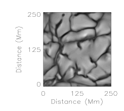
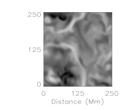
Figure 1: The vertical velocity in slices of the model convection zone in the initial state at two different depths: at the surface (left) and at the depth of the flux rope (right).

The computational box is horizontally periodic with sides of 250 Mm and a height of 313 Mm (of which 166 Mm is the convection zone, that covers 2.5 orders of magnitude in pressure). The flows are turbulent through-out the convection zone, and the kinetic energy spectrum displays a power law at intermediate wavenumbers ($k\approx$ 3 – 10). As it is typical for over-turning stratified convection, a cellular granulation pattern is generated on the surface of the convection zone (Fig. 1). The typical length scale of this pattern is about 50 Mm, somewhat larger than the canonical size of 32 Mm of solar super-granules (e.g. Leighton et al. Leighton+ea62 (1962)). The typical velocity of the granulation is 200 m/s in the narrow downdrafts at the surface and slightly less in the upwelling regions, close to what is found for solar super-granulation (e.g. Worden & Simon Worden+Simon76 (1976)).

We choose an initially isentropic flux rope with a buoyancy of $1/\gamma$ (with $\gamma=5/3$) lower than the case of temperature balance, where the buoyancy is $1/\beta$ (with $\beta$ being the classical plasma beta). This is computationally advantageous, since we avoid the costly process of perturbing the flux rope from a state of mechanical equilibrium.

The initial twist of the flux rope is given by

$$B_{z}=B_{0}e^{-(r/{\rm R})^{2}}\leavevmode\nobreak\ {\rm and}\leavevmode\nobreak\ B_{\phi}=\alpha(r/{\rm R})B_{z},$$ (5)

where $B_{z}$ is the parallel and $B_{\phi}$ the transverse component of the magnetic field with respect to the rope’s horizontal main axis. The coordinate system is chosen so that $z$ corresponds to the initial axial direction of the rope.

The wavelength $\lambda$ of the flux rope is equal to the horizontal size of the domain so that $\lambda=3.2\leavevmode\nobreak\ {\rm H}_{\rm P0}$ at the initial position of the rope. Thus, the flux rope is not undular Parker-unstable even though the stratification permits this instability for longer wavelengths (Spruit & van Ballegooijen Spruit+ea82 (1982)). The rope is initially twisted, with a pitch angle (at $r={\rm R}$) of $\psi_{\rm R}=\arctan(\alpha)$ and a radius ${\rm R}_{0}=0.177\leavevmode\nobreak\ {\rm H}_{\rm P0}$ which corresponds to a half-width at half-maximum of $B_{z}$ (henceforth HWHM) of $\sim 0.1\leavevmode\nobreak\ {\rm H}_{\rm P0}$.

To avoid problems associated with the large ratio of thermal to dynamic time scales, our convection model has a much higher luminosity than the Sun, and thus, all variables must be scaled to compare with solar values. The choice of the magnetic field strength is somewhat problematic in this regard. The ratio of kinetic to thermal energy density $e_{\rm K}/e$ is much larger in our model than in the Sun (though the convective flows remain subsonic with an average Mach number of 0.01). This requires a choice of $\beta$ that is smaller than its presumed value at the base of the solar convection zone so that the ratio of magnetic to kinetic energy density $e_{\rm M}/e_{\rm K}$ is the proper order of magnitude. However, a small $\beta$ is what is needed so that the time it takes to complete a simulation is not prohibitively long. We choose $\beta=100$, which yields a solar-like $e_{\rm M}/e_{\rm K}$ of 100.

3 Results

We have performed several fully convective 3-d simulations, as well as a number of 2-d convection-less simulations. The results of the latter agree with previous 2-d findings, and are used for reference in the following. We discuss results from a 3-d simulation with $\psi_{\rm R}=45^{\circ}$ ($\alpha=1$). In that case, the degree of twist is small enough to prevent the onset of the kink instability (the linear growth rate vanishes for $\alpha=1$, e.g. Fan et al. Fan+ea99 (1999)), yet it is large enough to prevent the onset of the Rayleigh-Taylor instability. Thus, the rope retains its cohesion without distorting its shape by any of these two instabilities, and we can focus our attention on the effects of the convective flows on the rope.

Figure 2: a) height of the flux rope as a function of time (stars). Also plotted are the corresponding results from a 2-d reference simulation (diamonds). The straight line corresponds to the average speed ($0.1\leavevmode\nobreak\ v_{\rm A0}$) in the rise phase. b) drift of the flux rope in the meridional plane. c) expansion of the flux rope (stars) with the corresponding result from the 2-d reference simulation over plotted (diamonds). Also plotted is an analytical expression (solid line, see text). d) magnetic field strength as a function of height.

Fig. 2 compares our 3-d simulation to a corresponding 2-d convection-less reference simulation, and a simple analytic flux tube. As the 3-d rope rises, convective flows perturb its motion, preventing it from entering a well-defined terminal rise phase with a constant rise speed, as in the 2-d reference simulation (see Fig. 2a). The rope remains straight and the maximum excursion of its axis, at the end of the simulation, is $\sim 0.04\leavevmode\nobreak\ \lambda$, where we define the rope’s axis as the set of positions along the rope, where the magnetic field strength is maximum. With the chosen super-equipartition axial field strength, the main action of the large-scale convective flows is to push the rope both left and right of the central plane (Fig. 2b; see also the mpeg-movie at Dorch Dorch-mpeg (2001)), while the effect of the small-scale downdrafts (of the order of the rope’s radius) is to locally deform its equipartition boundary.

Initially the rope is located in a general updraft region. This explains why the rise speed of the rope is slightly greater than that of the 2-d reference simulation, which reaches a terminal speed of $\sim 0.1\leavevmode\nobreak\ v_{\rm A0}$ ($v_{\rm A0}$ being the Alfvén speed at the initial position of the rope). Nevertheless, the two ropes arrive at the same final height at the end of the runs (though in the 3-d case, we note that the rope follows a longer path). Our 3-d rope also expands more quickly than the rope in the 2-d simulation, and its rate of expansion is closer to what is expected from an adiabatically expanding, non-stretching tube with constant flux ($B/\rho=$const.):

$${\rm R}(x)={\rm R}_{0}\left(1-\nabla_{a}\frac{x-x_{0}}{{\rm H}_{\rm P0}}\right)^{-1/2\nabla_{a}}.$$ (6)

Fig. 2c shows the rope’s characteristic size ${\rm R}_{hwhm}$ defined by the average between the vertical and horizontal HWHM along its axis (the short period oscillations due to differential buoyancy, that are not well-resolved, have been filtered out by smoothing over two grid points). As the rope rises and expands, its magnetic field strength ${\rm B}_{c}$, here defined as the average axial field strength along the rope, decreases at a rate close to that determined by Eq. (6). At later times, the field strength of the 3-d and 2-d ropes decrease at nearly the same rate (Fig. 2d). The deviation can be attributed to the fact that, during its ascent, a significant amount of the magnetic flux within the 3-d rope is lost to its surroundings.

Figure 3: Left: magnetic flux within the rope $\Phi_{i}$ (stars), the corresponding quantity in the 2-d simulation (diamonds) and an analytic fit (solid curve), Right: the normalized flux outside and above the center of the 3-d rope $\Phi_{u}$ (stars), and below, $\Phi_{l}$ (triangles). The same quantities are shown for the 2-d reference simulation (solid and dashed curves respectively).

This is illustrated by Fig. 3 (left), which shows the total normalized magnetic flux within the HWHM-boundary $\Phi_{i}$ as a function of time for both the 2-d and 3-d ropes. We note that as the 3-d simulation progresses, the total flux-loss from the computational domain is only 0.3$\%$. The flux content of the rope, however, decreases much more quickly.

Also shown in Fig. 3 (right) is the magnetic flux external $\Phi_{e}$ to the rope both above and below its center $\Phi_{u}$ and $\Phi_{l}$ respectively. Since the sum $\Phi_{e}+\Phi_{i}$ is nearly conserved, as $\Phi_{i}$ decreases, $\Phi_{e}=\Phi_{u}+\Phi_{l}$ must increase by an equal amount. However, the distribution of the flux-loss is not symmetric: more flux is lost to the surroundings below the rope than above. The e-folding time of the increase of flux $\Phi_{l}$ in the lower domain is $\sim 20\leavevmode\nobreak\ \tau_{\rm A}$ (with $\tau_{\rm A}={\rm R}_{0}/v_{\rm A0}$).

This asymmetry also exists in the 2-d reference simulation, even though the total flux-loss is much smaller in that case. The asymmetry is a result of two factors. First, as the rope rises, the total volume above it decreases, while the volume below it increases. Second, there is an anti-symmetry of the relative velocity across the rope. When the rope ascends, there is a tendency for flux to be advected towards the rope near its apex, and transported away from the rope in its wake. The more pronounced asymmetry in the 3-d case can be attributed to the pumping effect that transports the weak field downwards (Dorch & Nordlund Dorch+Nordlund01 (2001) and Tobias et al. Tobias+ea01 (2001)).

We have defined the flux rope as the magnetic structure that lies within the HWHM-boundary. This boundary is not, however, a contour that moves with the fluid in the classical sense: the flux within the latter kind of contour is naturally conserved (neglecting resistive effects) and equal to the total flux $\Phi_{0}=\Phi_{e}+\Phi_{i}$. The HWHM-boundary is a convenient way of defining the flux rope and a characteristic size ${\rm R}_{hwhm}$, that behaves more or less as it is expected from the analytical expression Eq. (6). The evolution of the flux within the rope’s core $\Phi_{i}$ is determined by

$$\dot{\Phi}_{i}=-\oint_{\rm boundary}\Delta{\bf v}\times{\bf B}\cdot{\rm d}{\bf l},$$ (7)

where $\Delta{\bf v}$ is the difference between the fluid velocity and the motion of the HWHM-boundary. The average “slip” $\overline{\Delta v}$ of the rope’s boundary in the simulation is only a small fraction of the rise speed, and varies between the range of plus or minus a few times $10^{-4}\leavevmode\nobreak\$ and $10^{-3}\leavevmode\nobreak\ v_{\rm A0}$.

Making the rather crude assumptions that the boundary only moves radially relative to the fluid and that the circumference of the boundary is circular (which it is not), Eq. (7) reduces to

$$\dot{\Phi}_{i}=-\pi{\rm R}_{hwhm}\leavevmode\nobreak\ \Delta v\leavevmode\nobreak\ {\rm B}_{c},$$ (8)

where ${\rm B}_{c}$ is the field strength at the center of the flux rope. Integrating Eq. (8) numerically with ${\rm R}_{hwhm}$ and ${\rm B}_{c}$ determined from the simulation (see Fig. 2), the result is a perhaps surprisingly good fit to the actual flux-loss, see Fig. 3 (left), if $\Delta v$ is set to 3 10${}^{-4}\leavevmode\nobreak\ v_{\rm A0}$ throughout the time span of the simulation except for a short interval of $\sim 3\leavevmode\nobreak\ \tau_{\rm A}$ around $t=30\leavevmode\nobreak\ \tau_{\rm A}$, where $\Delta v=-10^{-3}\leavevmode\nobreak\ v_{\rm A0}$, when the rope passes from one updraft to another (see the discussion below).

4 Discussion and conclusions

The 3-d numerical simulations show that the interaction of a buoyant twisted flux rope with stratified convection leads to a considerable loss of magnetic flux from the core of the flux rope (as defined by the rope’s HWHM-boundary).

The initial position of a flux rope in the convection zone is significant for the subsequent detailed history of its rise: with the present convective flows and the initial location of the flux rope, most of the rope starts out located inside or close to a convective updraft. Thus, the ascent of the rope is likely to be influenced by this fact, and we are therefore not able to draw any conclusions on the detailed path of its rise. However, in the course of the simulation, the flux rope rises 96 Mm, and loses about 25% of its original flux content. This, ceteris paribus, leads to an increase in the amount of toroidal flux that must be stored at the bottom of the convection zone during the course of the solar cycle.

In the Sun, toroidal flux ropes rise about 200 Mm through the convection zone before emerging as bipolar active regions. One may thus expect them to lose even more of their initial flux, which would then be pumped back down toward the bottom of the convection zone. We can quantify this subsequent flux-loss by assuming that Eq. (8) is valid through-out the rise, that the ropes expand according to the simple analytical estimate of Eq. (6), and that the ratio of the slip $\Delta v$ to the rise speed remains constant. Given these assumptions, the flux-loss at a height of 200 Mm is 26 % of the initial flux, i.e. not much more than in our simulation. However, the relative slip may not remain constant throughout the rope’s rise. For example, $\Delta v$ and thus $\dot{\Phi}_{i}$ changes at the time around $t=30\leavevmode\nobreak\ \tau_{\rm A}$, which corresponds to the time when the rope is at its maximum (rightward) excursion from a vertical ascent (see Fig. 2b). At that time, the rope exits the convective updraft with which it was initially associated, and enters a different ascending “plume” to the left of the its original position. This leads to a transient compression of the rope ($\Delta v<0$, in the simplified expression Eq. 8). After entering the new plume, the average slip returns to its previous positive value for the remainder of the rise.

Petrovay & Moreno-Insertis (Petrovay+Moreno97 (1997)) suggested that turbulent erosion of magnetic flux tubes may take place within the solar convection zone due to the “gnawing” of turbulent convection. They propose a mechanism whereby a flux tube is eroded by a thin current sheet that forms spontaneously within a diffusion time. That we do not see a loss of flux via this type of enhanced diffusion should not, however, be taken as a dis-proof of the feasibility of turbulent erosion: it requires the turbulence to be resolved down to much smaller scales $\ell\ll\lambda$, than in our simulations. Instead, the flux-loss is completely due to the advection of flux away from the core of the flux rope by convective motions. Most of the flux that is “gnawed-off” ends up in the trailing wake and some of this flux is mixed back into the upper layers by ascending flows. We speculate that both types of flux-loss may take place simultaneously in the Sun, and as a result, the amount of toroidal flux stored near the bottom of the solar convection zone may currently be underestimated.

- (1) Abbett, W.P., Fisher, G.H., and Fan, Y., 2000, ApJ 540, 548
- (2) Canfield, R.C., Hudson, H.S., and McKenzie, D.E ., 1999, Geoph. Res. Letters 26(6), 627
- (3) Caligari, P., Moreno-Insertis, F., and Schüssler, M., 1995, ApJ 441, 886
- (4) Cattaneo, F., Chiueh, T., and Hughes, D., 1990, JFM 219, 1
- (5) Dorch, S.B.F., 2001, www.astro.su.se/dorch/rope.mpg
- (6) Dorch, S.B.F. and Nordlund, Å., 1998, A&A 338, 329
- (7) Dorch, S.B.F., Archontis, V., and Nordlund, Å., 1999, A&A 352, L79
- (8) Dorch, S.B.F. and Nordlund, Å., 2001, A&A 365, 562
- (9) Emonet, T. and Moreno-Insertis, F., 1996, ApJ 458, 783
- (10) Emonet, T. and Moreno-Insertis, F., 1998, ApJ 492, 804
- (11) Fan, Y., Fisher, G.H., and McClymont, A.N., 1994, ApJ 436, 907
- (12) Fan, Y., Zweibel, E.G., Linton, M.G., and Fisher, G.H., 1999, ApJ 521, 460
- (13) Galsgaard, K. and Nordlund, Å., 1997, Journ. Geoph. Res. 102, 219
- (14) Leighton, R.B., Noyes, R.W., and Simon, G.W., 1962, ApJ 135, 474
- (15) Matsumoto, R., Tajima, T., Chou, W., Okubo, A., and Shibata, K., 1998, ApJ 493, L43
- (16) Matthews, P., Hughes, D., and Proctor, M.R.E., 1995, ApJ 448, 938
- (17) Moreno-Insertis, F., 1986, A&A 166, 291
- (18) Moreno-Insertis, F. and Emonet, T., 1996, ApJ 472, L53
- (19) Nordlund, A., Brandenburg, A., Jennings, R.L., Rieutord, M., Roukolainen, J., Stein, R.F., Tuominen, I., 1992, ApJ 392, 647
- (20) Petrovay, K. and Moreno-Insertis, F., ApJ 485, 398
- (21) Schüssler, M., 1979, A&A 71, 79
- (22) Spruit, H.C., 1981, A&A 98, 155
- (23) Spruit, H.C. and van Ballegooijen, A.A., 1982, A&A 106, 58
- (24) Sterling, A.C., Hudson, H.S., Thompson, B.J., and Zarro, D.M., 2000, ApJ 532, 628
- (25) Tobias, S.M., Brummell, N.H., Clune, T.L. and Toomre, J., 2001, ApJ 549, 1183
- (26) Tsinganos, K., 1980, ApJ 239, 746
- (27) Worden, S.P. and Simon, G.W., 1976, Solar Phys. 46, 73