Bias in Matter Power Spectra ?

We review the constraints given by the linear matter power spectra data on cosmological and bias parameters, comparing the data from the PSCz survey (Hamilton et al., 2000) and from the matter power spectrum infered by the study of Lyman alpha spectra at z=2.72 (Croft et al., 2000). We consider flat–$\Lambda$ cosmologies, allowing $\Lambda$, $H_{0}$ and $n$ to vary, and we also let the two ratio factors $r_{pscz}$ and $r_{lyman}$ ($r^{2}_{i}=\frac{P_{i}(k)}{P_{CMB}(k)}$) vary independently. Using a simple $\chi^{2}$ minimisation technique, we find confidence intervals on our parameters for each dataset and for a combined analysis. Letting the 5 parameters vary freely gives almost no constraints on cosmology, but requirement of a universal ratio for both datasets implies unacceptably low values of $H_{0}$ and $\Lambda$. Adding some reasonable priors on the cosmological parameters demonstrates that the power derived by the PSCz survey is higher by a factor $\sim 1.75$ compared to the power from the Lyman $\alpha$ forest survey.

1 Introduction

Bias, defined to be the ratio of rms luminosity density fluctuations to dark matter fluctuations at a fiducial scale of 12$h_{2/3}^{-1}$ Mpc, is the most uncertain of the minimal set of cosmological parameters. These may be taken to be $\Lambda$, $H_{0}$, $\Omega_{0}$ and $\Omega_{b}$ for the background, with the inhomogeneities described by $n$ and the bias parameter $b$.

There are three techniques available for computing the shape and amplitude of the power spectrum of density fluctuations. These involve using the CMB anisotropy data (BOOMERanG, MAXIMA, DASI), galaxy redshift surveys (PSCz, Hamilton & Tegmark, 2000) and the Lyman alpha forest (Croft et al., 2000). Use of large-scale peculiar velocity surveys and of galaxy cluster abundances provide a value of the normalisation, via the parameter $\sigma_{8}\Omega_{0}^{0.6}$, where $\sigma_{8}\equiv b$ evaluated at the fiducial scale of 12$h_{2/3}^{-1}$ Mpc. We confirm that CMB and galaxy surveys provide a consistent data set for the power spectrum. However incorporation of the matter power spectra inferred from Lyman alpha forest requires a relative bias of galaxies relative to the Lyman alpha forest once reasonable priors are adopted for the cosmological parameters.

Figure 1: Actual data set of matter power spectra. Up: PSCz spectrum. Down: Lyman alpha power spectrum. The solid line is the best model of the combined analysis (see text) and the (blue) dotted line correspond to the best model of the CMB, PSCz, Lyman $\alpha$ combined analysis.

2 Data sets

2.1 PSCz

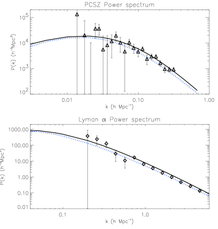
The linear power spectrum inferred by the PSCz survey is taken from Hamilton & Tegmark 2000 (HT00 hereafter). We choose the 22 points given in table B2 of HT00, which correspond to estimates of the decorrelated linear power spectrum. The dataset is shown in the upper part of figure 1.

2.2 Lyman $\alpha$

We use the linear matter power spectrum inferred from the flux power spectrum of lyman $\alpha$ forest spectra by Croft et al., 2000 (C00 hereafter). This corresponds to 13 estimates of the spectrum at $<z>=2.72$, referenced in table 4 of C00. When these data are used, the normalisation uncertainty (+27%, -23%) is included, then marginalised over (see next paragraph). The data are drawn in the lower part of figure 1.

3 Cosmologies

3.1 Free parameters

In this paper, we consider flat cosmologies, with no reionisation, no massive neutrinos and no tensor fluctuations. We also fix the baryon fraction to be consistent with Big–Bang nucleosynthesis and CMB determinations: $\Omega_{b}h^{2}=0.020$. The remaining parameters are listed in table 1, as well as the corresponding ranges and steps. All the theoretical power spectra are COBE–normalised, and the ratio parameters are defined as:

$$P(k)_{pscz/lyman}=r_{pscz/lyman}^{2}P_{cmb}(k).$$

Here $\lambda_{\rm o}$ is the vacuum density and $n$ is the fluctuation spectral index.

	$H_{\rm o}\ kms^{-1}/Mpc$	$\lambda_{\rm o}$	$n$	$r_{pscz}$	$r_{lyman}$
Min.	20	0.0	0.70	0.50	0.10
Max.	100	1.0	1.30	1.475	2.05
step	10	0.1	0.03	0.025	0.05

Table 1: Parameter space explored:

$\Omega_{\rm tot}=1$
$\Omega_{b}h^{2}=0.020$

3.2 Theoretical matter power spectrum

We have considered theoretical matter power spectra with an arbitrary value of the shape parameter ($\Gamma$), using the approach of Bardeen (1986) and Sugiyama (1995). We computed the COBE normalisation of the spectra using the CAMB (Lewis, Challinor, & Lasenby (2000)) code. We used the “grow package” from Hamilton 2001 to derive the growth factor. Our two theoretical power spectra at z=0 and z=2.7 are presented in the following equations:

$$P_{z=0}(k) = N_{1}\times TF(\Gamma,k)^{2}\times g(\Lambda)^{2}\times P_{o}(k)*r_{pscz}^{2}$$ (1)

$$P_{z=2.72}(k) = N_{2}\times f_{z}\times TF(\Gamma,k)^{2}\times g(\Lambda)^{2}\times P_{o}(k)*r_{lyman}^{2}$$ (2)

where we write:

$$f_{z}=(1+z)^{-2}*[(\Lambda+\Omega_{m}*(1.+z)^{3}+\Omega_{k}*(1+z)^{2})^{1/2}]^{3}$$ (3)

and the initial matter power spectrum is given by:

$$P_{o}(k)=(k*h)^{n}$$ (4)

We take the transfer function to be:

$$TF(\Gamma,k)=\frac{ln(1+2.34*q)}{(2.34*q)}\times$$

$$\frac{1}{(1+\alpha_{2}*q+(\alpha_{3}*q)^{2}+(\alpha_{4}*q)^{3}+(\alpha_{5}*q)^{4})^{1/4}}$$ (5)

where $q=k/\Gamma$. We use the coefficients given by Sugiyama (1995): $\alpha_{1}=2.34,\ \alpha_{2}=3.89,\ \alpha_{3}=16.1,\ \alpha_{4}=5.46,\ \alpha_{5}=6.719$. Here we treat $\Gamma$ as a free parameter. We then marginalize over it. The shape of the power spectrum will be investigated in a future paper. $N_{1}$ and $N_{2}$ are normalisation factors, such that our matter power spectra are COBE–normalised.

4 Statistics

4.1 Likelihood

We approximate the likelihood functions of our parameters by independent multivariate Gaussians, using the following expression:

$$\mathcal{L}_{pscz/lyman}=exp-\frac{\chi^{2}_{pscz/lyman}}{2}$$

For the PSCz data, the $\chi^{2}$ has been computed as follows:

$$\chi^{2}_{pscz}(\Theta_{p})=\sum\frac{(P_{i}(k_{i})-P^{model}(\Theta_{p}|k_{i}))^{2}}{\sigma_{i}^{2}.}$$ (6)

where $P^{model}$ is derived from equation 1 of the following section and $\Theta_{p}$ is the set of parameters explored listed in table 1.

Concerning the Lyman alpha data, we take into consideration the uncertainty on the normalisation. We add a contribution to $\chi^{2}$, assuming a double–tail Gaussian for the normalisation distribution:

$$\hat{\chi}^{2}_{lyman}(\Theta_{l},N)=\sum\frac{(P_{i}(k_{i})-P(\Theta_{l},N|k_{i})^{2}}{\sigma_{i}^{2}.}$$

$$+\frac{(N-1.)^{2}.}{(\sigma^{2})}$$

$$\chi^{2}_{lyman}(\Theta_{l})\equiv-2\times\log\left[\int exp(-\frac{\hat{\chi}^{2}_{lyman}}{2})dN\right]$$ (7)

4.2 Results

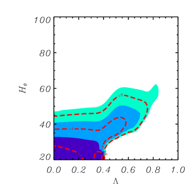
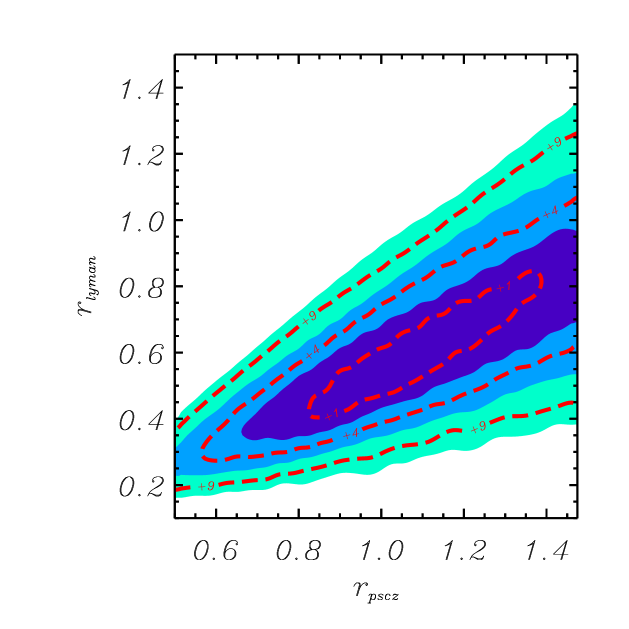
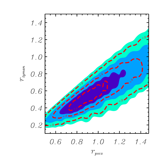
The results are shown in 2D contours plots, with red-dashed lines corresponding to confidence intervals 68, 95, 99% in one dimension, and filled contours corresponding to 68, 95, 99% in two dimensions. The remaining parameters have been marginalised (not integrated), finding the minimum for each pair of parameters plotted in the graphs.

5 Results and constraints

5.1 PSCz and Lyman $\alpha$ matter spectra

Given our 5 free parameters, the constraints given by each set independently are almost inexistent. Many combinations of parameters lead to degeneracies which allow values even out of our grid of parameters.

5.2 Are the two data sets consistent ?

We have seen that our two data sets allow most of the values for the parameters we are considering. Nevertheless, this does not mean that they are compatible. Marginalising over parameters, for a better view of the constraints, does not allow us to include all the correlations and degeneracies between parameters. This is even more critical when the constraints are weak. To see whether the data are consistent in some particular cosmologies, we adopt two scenario. The first is to consider that the ratios are the same for both datasets. Marginalising over these will reveal the prefered range for the cosmological parameters. The second approach is to let the ratios vary freely, while putting some priors on the cosmological parameters. This will give us estimates of the ratio for each data set.

5.2.1 Uniform ratio

We have combined the data sets by adding the two $\chi^{2}$ grids defined in equations 6 and 4.1, $r$ being the unique bias parameter. The prefered models obtained with this assumption correspond to very low values of $H_{o}$ and $\Lambda$. The “best one” is plotted in figure 1. The value of the goodness of fit for this model, given by the absolute value of the $\chi^{2}$ on the two dataset, is good ($\chi^{2}_{min}=22$ for 30 degrees of freedom). The corresponding confidence intervals are shown in figure 2, where the remaining parameters have been marginalised over. This combined analysis give strong constraints on the cosmological parameters, which are largely in contradiction with most estimates of the cosmological parameters from independent techniques (such as SNIa, age of the Unviverse, CMB). Although the concordance model is marginally acceptable, a low $H_{0}$ tilted CDM model is preferred.

Figure 2: Combined constraints from the Lyman $\alpha$ power spectrum and the PSCz spectrum with the same ratio. Filled contours mark the 68, 95 and 99% confidence levels in 2–dimensional space. The dashed red line define the 68, 95 and 99% confidence levels when projected on 1 parameter.

5.2.2 Ratio parameters

The preceding discussion does not reinforce our faith in the concordance model with respect to other parameter estimates. The analysis of the data could be done via an alternative approach. Assuming that we “know” the cosmological parameters, we may examine the relative bias of the two data sets. Statistically speaking, this means that we can put priors on the cosmological parameters, marginalise over them, and see what the constraints are on the 2 remaining parameters that are associated with the inhomogeneities power. We adopt the reasonable following priors in our analysis: $\Lambda=0.7\pm 0.1$, $H_{0}=65\pm 10\ kms^{-1}Mpc^{-1}$, $n=1\pm 0.1$ which are in agreement with most of the actual parameter estimates in the literature. We assume a Gaussian shape for the priors, giving the following likelihood:

$$\hat{\chi}^{2} = \chi^{2}_{pscz}+\chi^{2}_{lyman}+\chi^{2}(\Lambda)+\chi^{2}(H_{0})+\chi^{2}(n)$$

$$\chi^{2}(\Lambda) = \frac{(\Lambda-0.7)^{2}}{0.1^{2}}$$

$$\chi^{2}(H_{0}) = \frac{(H_{0}-65)^{2}}{10^{2}}$$

$$\chi^{2}(n) = \frac{(n-1.0)^{2}}{0.1^{2}}$$

then

$$\chi^{2}_{combined}(r_{pscz},r_{lyman})=Min_{[\Lambda,H_{0},n]}(\hat{\chi}^{2})$$ (8)

Figure 3 shows the confidence intervals for $r_{pscz}$ and $r_{lyman}$. The best model is obtained for $r_{pscz}=1.075$ and $r_{lyman}=0.6$, with a good goodness of fit: $\chi^{2}=24.8$ for 29 degrees of freedom. We can clearly see, in the figure 3 the correlation between the two biases that leads to a relation (over the explored range of parameters and between the 95% confidence level interval):

$$r_{pscz}=1.57*r_{lyman}+0.16\;\;\;or\;\;\;\frac{r_{pscz}}{r_{lyman}}\sim 1.8$$ (9)

The corresponding 68% intervals on each ratio are: $0.45<r_{lyman}<0.8$ and $0.8<r_{lyman}<1.35$; the constraints being low at 95% CL.

Figure 3: Combined Constraints from the Lyman $\alpha$ matter power spectrum and the PSCz spectrum with priors on cosmological parameters (see text)

5.2.3 Combining CMB and matter spectra

Figure 4: CMB constraints using COBE, BOOMERanG, DASI and MAXIMA datasets for flat $\Omega_{b}h^{2}=0.02$ models.

Figure 5: Combined Constraints from CMB, PSCz spectrum and the Lyman $\alpha$ power spectrum in the ($r_{pscz},r_{lyman}$) plane

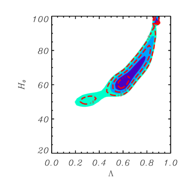
Instead of setting independent priors on each cosmological parameter, we can use the latest CMB analysis as a prior. In LeDour et al., 2000 and Douspis et al., 2001, we used the current CMB data set to derive constraints on cosmological parameters. The latter paper considers the most recent data including BOOMERanG (Netterfield et al., 2001), DASI (Halverson et al., 2001) and MAXIMA (Lee et al., 2001). We use the same grid as in table 1 for the CMB analysis. As seen in the literature (Douspis 2000, Jaffe et al., 2001, Melchiorri and Griffiths, 2000 and others), the CMB by itself does not constrain $H_{0}$ or $\Lambda$; both of these parameters are degenerated with the total density (or the curvature). As we have fixed $\Omega_{b}h^{2}=0.02$ and $\Omega_{total}=1$ in this analysis, the CMB now gives interesting confidence intervals on the remaining cosmological parameters (see figure 4). These constraints are similar to those used in the previous section, but contain more information, because of the correlations between parameters. This way of setting priors should be preferable to the previous one.

We constructed a new likelihood grid from the CMB and the matter power spectra:

$$\chi^{2}(\theta) = \mathcal{A}_{cmb}+\chi^{2}_{pscz}+\chi^{2}_{lyman}$$ (10)

$$\rm with\;\;\;\theta = (\Lambda,H_{0},n,\Gamma,r_{pscz},r_{lyman})$$ (11)

where $\mathcal{A}$ is the approximation developed in Bartlett et al., 2000. We then maximise this new grid and marginalise to find confidence intervals. The best model given by $\Lambda=0.6,\ H_{0}=60,\ n=0.97,\ \ r_{pscz}=0.875,\ r_{lyman}=0.5$ has a good goodness of fit and is plotted in figure 1.

As the constraints on cosmological parameters are stronger in the CMB analysis than in the matter power spectrum analysis, we do not expect any improvement on cosmological parameter confidence intervals. On the other hand, marginalising over $\Lambda,\ H_{0},\ n$ gives us interesting constraints on $r_{pscz}\ {\rm and}\ r_{lyman}$. When the three datasets are combined, we find constraints on the relative bias and again a degenerated relation between the two ratio parameters, leading to a lower ratio factor for the Lyman linear power spectrum (cf figure 5). The 68 % confidence level are the following: $0.45<r_{lyman}<0.6$ and $0.7<r_{lyman}<1.1$. We may also express the relative bias between the two sets of data as:

$$r_{pscz}=1.33*r_{lyman}+0.20\;\;\;or\;\;\;\frac{r_{pscz}}{r_{lyman}}\sim 1.75$$ (12)

inside the 95% confidence levels.

6 Conclusions

Determination of the cosmological model parameters is entering into a new era of precision. The weakest link in our understanding of the universe is in the realm of the density fluctuations, and their evolution. It is well known that bias depends on the objects being sampled, and varies with galaxy luminosity and morphological type. However these variations are attributed to the complex physics of galaxy formation. We find here that by adopting reasonable cosmological model priors, the matter power spectrum inferred by Lyman alpha forest power spectrum can be shown to be biased low relative to the the bias of $L_{\ast}$ galaxies.

It is usually assumed that the Lyman alpha forest, representing gas that has not yet virialized and has density contrast between unity and 200, is a good tracer of the dark matter (e.g. Croft et al. 2001). In fact this is a dangerous assumption, since the Lyman alpha forest gas is a very small fraction of the total gas density, 99.99 percent or more of which is ionized. Moreover, the proximity effect observed for quasars and more recently for Lyman break galaxies (Steidel 2001), demonstrates that the forest is not a good tracer of the total matter density on scales of up to tens of megaparsecs.

We note that gas-rich dwarf galaxies, which avoid the vicinities of luminous galaxies, also display a significantly lower bias, or even an antibias, compared to that of luminous galaxies. Dwarfs are likely to be the final fate of much of the forest. Indeed LCDM simulations of clustering find that luminous galaxies themselves are somewhat antibiased. Hence our result fits in well with hierarchical structure formation, since the low Lyman alpha forest ratio $\frac{r_{pscz}}{r_{lyman}}\sim 1.75$ is similar to that of dwarf galaxies.

References

- Bardeen (1986) Bardeen et al., 1986, ApJ, 304, 15
- Bartlett, Douspis, Blanchard, & Le Dour (2000) Bartlett, J. G., Douspis, M., Blanchard, A., & Le Dour, M. 2000, A&AS, 146, 507
- Croft et al. (2000) Croft, R.A.C. et al., astro-ph/0012324
- Douspis (2000) Douspis, M., 2000, PhD thesis
- Douspis et al (2001) Douspis M., Blanchard A., Sadat R., Bartlett, J.G.,& Le Dour M., A&A in press, astro-ph/0105129
- (6) Halverson et al., astro–ph/0104489 (DASI)
- (7) Hamilton, A. J. S. 2001, MNRAS, 322, 419
- Hamilton & Tegmark (2000) Hamilton, A.J.S. & Tegmark, M., astro-ph/0008392
- Jaffe et al (2001) Jaffe et al. 2001, Phys. Rev. Lett., 86, 3475-3479
- Le Dour, Douspis, Bartlett, & Blanchard (2000) Le Dour, M., Douspis, M., Bartlett, J. G., & Blanchard, A. 2000, A&A, 364, 369
- (11) Lee et al., astro–ph/0104459 (MAXIMA)
- Lewis, Challinor, & Lasenby (2000) Lewis, A., Challinor, A., & Lasenby, A. 2000, ApJ, 538, 473
- (13) Melchiorri A. & Griffiths L.M., New Astronomy Reviews, 45, Issue 4-5, 2001
- (14) Netterfield et al., astro–ph/0104460 (BOOMERanG)
- Seljak & Zaldarriaga (1996) Seljak U. & Zaldarriaga M. 1996, ApJ 469, 437
- (16) Steidel C., 2001, private communication
- Sugiyama (1995) Sugiyama, N. 1995, ApJS, 100, 281