Interstellar Turbulence:
II. Energy Spectra of Molecular Regions in the Outer Galaxy

Abstract

The multivariate tool of Principal Component Analysis (PCA) is applied to 23 fields in the FCRAO CO Survey of the Outer Galaxy. PCA enables the identification of line profile differences which are assumed to be generated from fluctuations within a turbulent velocity field. The variation of these velocity differences with spatial scale within a molecular region is described by a singular power law, ${\delta}v=cL^{\alpha}$ which can be used as a powerful diagnostic to turbulent motions. For the ensemble of 23 fields, we find a mean value $<\alpha>$=0.62$\pm$0.11. From a recent calibration of this method using fractal Brownian motion simulations (Brunt & Heyer 2001), the measured velocity difference-size relationship corresponds to an energy spectrum, $E(k)$, which varies as k^-β, where $\beta=2.17\pm 0.31$. We compare our results to both decaying and forced hydrodynamic simulations of turbulence. We conclude that energy must be continually injected into the regions to replenish that lost by dissipative processes such as shocks. The absence of large, widely distributed shocks within the targeted fields suggests that the energy is injected at spatial scales less than several pc.

1 Introduction

Complex velocity fields and non-thermal line widths attest to the presence of turbulent flows in dense, molecular clouds. The energy density associated with such flows may provide the overall dynamical support to counter the self-gravity of molecular clouds and the pressure of the external medium and therefore, regulates the formation of stars in the Galaxy (Zuckerman & Evans 1974). For compressible gas, the advection of material through a chaotic velocity field contributes to the hierarchical structure of the dense interstellar medium (Falgarone, Phillips, & Walker 1991). While such dynamical functions have long been assigned to turbulence, there are few observational descriptions of the physical nature of such flows. Such descriptions are essential to a more complete accounting of the star formation process.

Since the instantaneous behavior of turbulent flows is unpredictable, most theoretical descriptions of turbulence focus upon statistical correlations of the velocity field (Landau and Lifshitz 1959). The energy spectrum, E(k), defined as the angular integral of the power spectrum of the velocity field, quantifies the degree to which the velocities are correlated with spatial scale. Over the inertial range of spatial scales, the energy spectrum varies as a singular power law with wave vector k,

$$E(k)\sim k^{-\beta}$$

The scaling exponent, $\beta$, provides a concise description of the velocity field and can be used to distinguish between different turbulent conditions. For example, the incompressible energy cascade model of Kolmogorov (1941) gives $\beta=5/3$. For compressible turbulent flows in which energy is dissipated in ubiquitous shocks, $\beta=2$ (Passot, Pouquet, & Woodward 1988; Passot, Vazquez-Semadeni, & Pouquet 1995; Gammie & Ostriker 1996). The functional form of the energy spectrum in equation 1.1 is equivalent to the statement that the root mean square velocity varies with size $l$ over which it is measured as

$$<v_{l}^{2}>^{1/2}\sim l^{\gamma}$$

where $\gamma=(\beta-1)/2$.

In principle, values of $\beta$ applicable to the molecular interstellar medium are constrained by observations. In practice, retrieving such dynamical information from spectroscopic imaging observations is challenging. Observed radiation fields lie on a fundamentally different basis than the intrinsic physical fields. Both real and modeled interstellar clouds are described by physical fields of velocity, v(x,y,z), density, n(x,y,z), temperature, T(x,y,z), molecular abundance, and the local UV radiation field, where x,y,z are spatial coordinates. Observed radiation fields, T_R(x,y,v_z), of a given molecular line transition are retrieved on the basis of projected position on the sky (x,y) and the Doppler-shifted line of sight velocity (v_z). Moreover, the radiation temperature field is an extremely complicated convolution of velocity, density, temperature and optical depth structure along the line of sight. If the velocity field is turbulent, involving multiple non-local re-correlations along the line of sight, then the transformation of the field to an axis is highly non-linear.

Several studies have shown that the observed molecular line profiles are incompatible with extreme values of $\beta$ (Goldreich & Kwan 1974; Leung & Lizst 1976; Dickman 1985; Kwan & Sanders 1986). That is, the velocity field is neither smooth ($\beta>3$) nor micro-turbulent ($\beta<1$). More direct measures of $\beta$ include “cloud-finding” decompositions from which a size-line width relationship is identified (Carr 1987; Stützki & Güsten 1990) and autocorrelation function and structure function analyses of centroid velocity fluctuations (Scalo 1984; Kleiner & Dickman 1985; Miesch & Bally 1994). While these analyses are widely used, there has been no demonstration that these methods can accurately recover the statistics, (i.e. $\beta$ or equivalently, $\gamma$), of molecular cloud velocity fields from radiation temperature (T_R(x,y,v_z)) measurements over a wide range of conditions. More recent efforts to exploit the three dimensional information within the observed data cubes include Rosolowsky et al. (1999) and Lazarian & Pogosyan (2000).

Heyer and Schloerb (1997) have applied the multivariate technique of Principal Component Analysis (PCA) to decompose spectroscopic imaging observations of targeted molecular regions. The effect of the decomposition is to identify velocity gradients over various scales as these are measured by differences within the line profiles with respect to the noise and resolution limits. From the set of significant eigenvector and eigenimages, they derive a power law relationship between the velocity differences and the spatial scale over which these gradients occur such that

$${\delta}v\sim L^{\alpha}$$

In a companion paper, Brunt & Heyer (2001) demonstrate that the method outlined by Heyer & Schloerb (1997) with some modifications, is sensitive to velocity fields with varying statistics and provide a calibration to estimate $\beta$ from the observed power law index $\alpha$ under a wide variety of physical and observing conditions. The basic calibration is $\beta=3{\alpha}+0.15$. We stress that this calibration was obtained under highly idealized conditions, using simulated observations generated from fractional Brownian motion (fBm) velocity fields and multifractal density fields, as described in Brunt & Heyer (2001). While such a calibration allows statistically controlled inputs to the calibration, it does not include features expected in real turbulent fields, such as intermittency or correlations between velocity convergences and density enhancements. For observational concerns, Brunt & Heyer (2001) found that PCA was not strongly affected by emission saturation, which may be expected to be present in the ¹²CO (J=1–0) data utilized here. The reasons for this are not completely understood, since the PCA method is currently empirical in nature. Self-reversal, we expect, would have an impact, but this was not prevalent in the simulated observations, nor is it widely seen in ¹²CO (J=1–0) emission. These points are discussed in more detail in $\S$4.

In this paper, we apply the PCA method to an ensemble of molecular regions to determine the degree of velocity correlation within the interstellar medium. The fields are extracted from the FCRAO CO Survey of the Outer Galaxy (Heyer et al. 1998). In $\S$2, we describe how the regions were selected. The analysis method is demonstrated in detail for one of the targeted regions in $\S$3. A summary of the analysis upon all of the fields is presented in $\S$4. In $\S$5, we discuss the results in context with phenomenological descriptions and hydrodynamic simulations of interstellar turbulence.

2 The Data

The FCRAO CO Survey of the Outer Galaxy is a spectroscopic imaging survey of molecular ¹²CO emission over a very large region of the outer Galaxy ($40^{\circ}\times 8^{\circ}$, sampled every $50\arcsec$) and covering the V_LSR  range -150 to +40 km s^-1  sampled every 0.81 km s^-1  (Heyer et al. 1998). The wide field and spatial dynamic range provide an unbiased sample of molecular emission and enable the isolation of a large number of fields to analyze.

2.1 Selected Fields

Twenty three fields have been selected from the Outer Galaxy Survey with a broad range of cloud morphologies. Nine of the fields are within the Perseus spiral arm defined here spectroscopically as $-60<V_{LSR}<-30$ km s^-1. The remaining fields have centroid velocities greater than -20 km s^-1  and are referred to collectively as “local” fields. Several well-known giant molecular clouds, both in the Perseus and local arms are included in the sample. These include clouds associated with optical and radio HII regions and OB associations (W3, W5, NGC 7538, and Sh 156, and Cep OB3). Fields were visually selected from inspection of spectroscopically-restricted integrated intensity maps and spatially-restricted global spectrum plots. In some cases, due to the angular limits of the Survey or due to the imposition of spectroscopic segregation, the emission does not fall to the zero level at the boundaries for some fields. This feature is mostly restricted to the local emission, which covers a broader range in Galactic latitude and suffers more from spectroscopic blending. Tests have been carried out to gauge the effect of truncating a region and suggest that it does not cause any significant problems since we are primarily interested in the statistics of the fields which are well sampled by the available spectra.

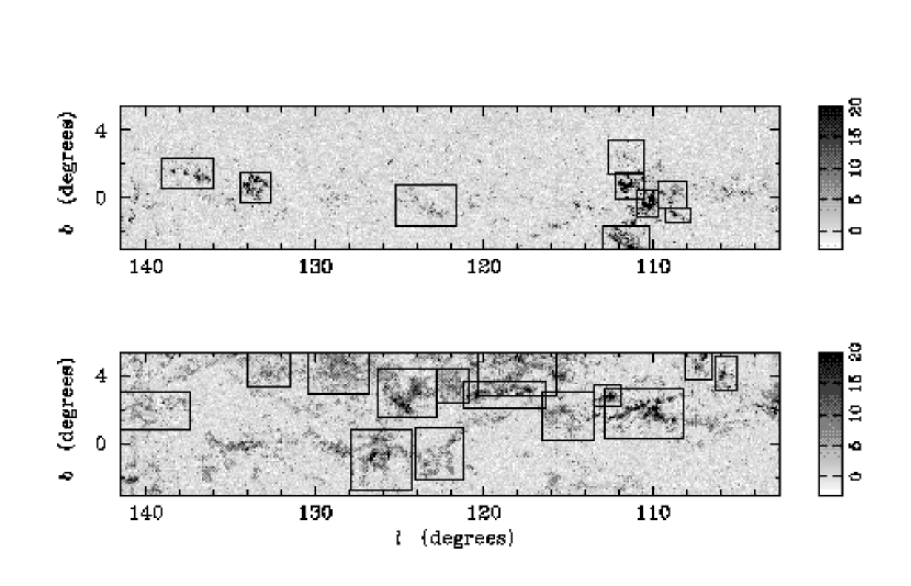
Figure 1: Images of ¹²CO J=1-0 intensity integrated over the velocity intervals of the Perseus (top) and local (bottom) spiral arms. The boxes show the individual fields analyzed in this study.

An overview of the selected fields is presented in Figure 1. The spectroscopic and angular limits ($v_{min}$:$v_{max}$, $l_{min}$:$l_{max}$, $b_{min}$:$b_{max}$), the number of spectroscopic channels (N_v) and spatial pixels (N_l $\times$ N_b) of these fields are reported in Table 1. To identify these fields in Figure 1, the identification number of the Perseus Arm (P) and local (L) fields increases with decreasing $l_{max}$. To obtain absolute spatial scales, kinematic distances have been derived from the velocity and positional centroids in each field assuming a flat rotation curve with V_∘ = 220 kms^-1 and R_∘ = 8.5 kpc. The derived scaling exponent, $\alpha$, is independent of distance while the amplitude, ${\delta}v$(1pc), is linearly dependent upon the presumed distance to the source. In this study, we are exclusively interested in $\alpha$.

3 Results

3.1 A Detailed Example of the Analysis

The formal description of PCA is presented by Heyer & Schloerb (1997) and Brunt & Heyer (2001). Here, we provide a detailed example of the complete analysis upon an individual field to demonstrate the statistical output from PCA and the extraction of characteristic scales from the set of eigenimages and eigenvectors. Given a data set $T(x_{i},y_{i},v_{j})=T_{ij}$ with n=$N_{l}{\times}N_{b}$ spectra and P spectroscopic channels, a set of P eigenvectors, $u_{l}$, and eigenvalues, $\lambda_{l}$, are derived from the solution of the eigenvalue equation with the covariance matrix, S, of the data,

$$Su=\lambda u$$

where

$$S_{jk}={{1}\over{n}}\sum_{i=1}^{n}T_{ij}T_{ik}$$

The eigenvectors are subject to the orthogonal condition,

$$\sum_{j=1}^{P}u_{jl}u_{jm}=\left\{\begin{array}[]{ll}1&\mbox{ if $l=m$}\\ 0&\mbox{ if $l{\neq}m$}\end{array}\right\}$$

The eigenvalues are equivalent to the variance of the data projected onto the respective eigenvectors. The eigenvalues and corresponding eigenvectors are sorted from largest to smallest to establish the principal components of the data set. An eigenimage, $I_{l}$, is constructed by projecting each spectrum in the field onto the $l^{th}$ eigenvector, $u_{l}$,

$$I_{l}(x_{i},y_{i})=I_{l}(r_{i})=\sum_{j=1}^{P}T_{ij}u_{jl}$$

Effectively, a given eigenvector, $u_{l}$, defines a spectral window with a characteristic velocity, ${\delta}v_{l}$, which gauges the profile differences over the observed field. The spectra are weighted by $u_{l}$ to produce a spatial map, $I_{l}(r)$, which locates line profile differences within the data cube. The first principal component generally consolidates all of the spectroscopic channels with signal. Higher order components ($l\approx P$) provide an accurate measure of the variance due to the random noise of the data. The equivalence of the eigenvalues with the projected variance enables a simple characterization of the signal to noise ratio of the data cube,

$$\zeta_{1}=\sqrt{{\lambda_{1}-\lambda_{P}}\over{\lambda_{P}}}$$

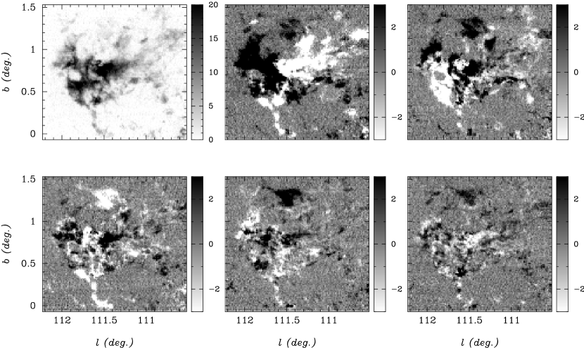
Figure 3: b) The set of eigenimages, $I_{l}(r)$, derived for the P6 field from the projection of the spectra onto the eigenvectors.

In Figure 2 and Figure 3, the set of eigenvectors and eigenimages derived for field P6 (NGC 7538) are shown. The first 3 components ($l=1,2,3$) identify the large scale kinematics of the cloud which is comprised of 2 features at velocities -56 and -50 km s^-1  respectively. Subsequent components ($l=4,5,6$) isolate smaller velocity differences within these features as these contribute to the measured variance of the data cube. Finally, for $l\geq 8$, any variance due to cloud kinematics can not be distinguished from the random noise of the data. Therefore, for this cloud, we need only to consider components $l<8$.

The identification of smaller velocity differences by the eigenvectors with increasing $l$ is intrinsic to the use of orthogonal functions to decompose the data cube. However, the spatial granularity of the eigenimages also decreases with increasing $l$ and reflects a fundamental property of spectral line observations of the molecular gas component in which line profiles are increasingly similar in shape and velocity with decreasing angular distances. It is this variation of spatial granularity with decreasing velocity which we wish to quantify as this is related to the energy spectrum of the velocity field (Brunt & Heyer 2001).

To determine the characteristic velocity and spatial scales for each component, the raw autocorrelation functions, $C_{V}^{l}(dv)$, $C_{I}^{l}(\tau)$, are calculated from the eigenvectors and eigenimages respectively,

$$C_{V}^{l}(dv)=<(u^{l}(v)u^{l}(v+dv)>$$

$$C_{I}^{l}(\tau)=<(I^{l}(r)I^{l}(r+\tau)>$$

where $\tau=\tau(x,y)$ These expressions include an additive component, $C_{N}(\tau)$ due to instrumental noise (Brunt & Heyer 2001). The noise subtracted autocorrelation function, $C_{I0}(\tau)$ is calculated,

$$C_{I0}(\tau)=C_{I}(\tau)-C_{N}(\tau)$$

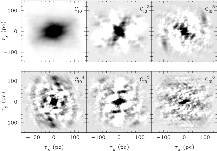
Figure 5: b) The 2D autocorrelation functions, $C^{l}_{I0}(\tau_{x},\tau_{y})$ of the eigenimages of the P6 field. The characteristic spatial scale, $L_{l}$, is derived for each principal component, $l$, from the e-folding lengths of $C^{l}_{I0}(\tau_{x},\tau_{y})$ respectively along the cardinal directions.

Since the 2 dimensional autocorrelation function is derived from a large number of lags, the noise contribution can be significant. Moreover, for spectroscopic data cubes constructed using reference sharing or on the fly mapping modes, the noise is correlated between positions observed with the same receiver horn and reference position. In these cases, $C_{N}(\tau)\neq 0$ for $\tau\neq 0$. The details to deriving $C_{N}(\tau)$ are discussed in the Appendix. The noise subtracted autocorrelation functions determined from the set of eigenvectors and eigenimages displayed in Figure 2 and Figure 3 are shown in Figure 4 and Figure 5 respectively.

The characteristic velocity scale, ${\delta}v_{l}$, is determined from the velocity lag at which

$$C_{V}^{l}({\delta}v_{l})/C_{V}^{l}(0)=e^{-1}$$

For the 2 dimensional ACF of the eigenimage, one must additionally correct for the effects of finite resolution observations upon the zero lag (see Brunt & Heyer 2001). We determine the spatial correlation lengths along the cardinal directions, ${\delta}x_{l},{\delta}y_{l}$, from the noise corrected ACF,

$${{C_{I0}^{l}({\delta}x_{l},0)}\over{C_{I0}^{l}(0,0)}}=e^{-1}$$

$${{C_{I0}^{l}(0,{\delta}y_{l})}\over{C_{I0}^{l}}(0,0)}=e^{-1}$$

and assign the biased characteristic spatial scale, $L_{lB}$ to the quadrature sum,

$$L_{lB}=\sqrt{{\delta}x_{l}^{2}+{\delta}y_{l}^{2}}$$

The true characteristic scale, $L_{l}$, is derived from $L_{lB}$ with subpixel corrections to account for finite resolution of the observations. Since the eigenimages tend to be isotropic, the ACF profiles along the cardinal directions are a reasonable approximation to the variation of the ACF along any arbitrary angle. The characteristic velocity and spatial scales are statistically well defined with respect to the noise as these represent mean values over the full spectrum and field respectively. A measurement error, $\sigma_{{\delta}v}$, to the value ${\delta}v_{l}$ is given by one half the velocity resolution of the spectrometer. For the spatial scale, $\sigma_{L}$ is determined from the quadrature sum of the spatial resolution and the degree of anisotropy, $|{\delta}x_{l}-{\delta}y_{l}|$, in the spatial ACF. The PCA velocity statistic, $\alpha$, is then obtained from the set of ${\delta}v,L$ pairs which are larger than the respective spectral and pixel resolution limits and form the power law relationship

$${\delta}v\propto L^{\alpha}$$

where the unsubscripted quantities refer to the ensemble (${\delta}v_{l},L_{l}$). The retrieval of each ${\delta}v,L$ pair represents a vast amount of information consolidated from the entire field and describes the spatial scales over which velocity gradients are detected as line profile differences. The set of (${\delta}v$, L) points derived from the significant principal components are plotted in Figure 6. A power law fit to these points yields a scaling exponent $\alpha=0.69\pm 0.02$.

3.2 Results for All Targeted Fields

Individual plots of the retrieved characteristic scale measurements for the selected fields are shown in Figure 6 and Figure 7. Power law fits to these relationships yield the scaling exponent, $\alpha$ and the amplitude, $c={\delta}v(1pc)$. These values are listed in Table 2 in addition to the number of principal components included in the fit (N_pc), the number of principal components rejected (N_c - see Brunt 1999), and the variance-based signal-to-noise estimates ($\zeta_{1}$). Values of $\gamma$ and $\beta$ which describe the intrinsic velocity field statistics have been derived according to the calibration of Brunt & Heyer (2001) and are also tabulated in Table 2. The error estimates listed for these values include all fitting errors and calibration uncertainties.

A summary of the derived values for $\alpha$ and $\beta$ is presented as a histogram in Figure 8. The shaded part of the histogram includes those regions with associated HII regions and OB stars. We have calculated weighted (1/$\sigma_{\alpha}^{2}$, where $\sigma_{\alpha}$ is the statistical uncertainty in the scaling exponent) and unweighted averages of the exponents reported in Table 2. The weighted values are: $<\alpha>=0.62\pm 0.11$, $<\beta>=2.17\pm 0.31$ , $<\gamma>=0.49\pm 0.16$. The unweighted values are: $<\alpha>=0.68\pm 0.10$, $<\beta>=2.21\pm 0.31$, $<\gamma>=0.57\pm 0.13$. The uncertainties of these derived averages are larger than those of the individual fits. The range in $\gamma$ is comparable to the range found by centroid velocity ACF analysis (see Miesch and Bally 1994).

There is no general relationship between the measured value of $\alpha$ and any subjectively assigned morphology of the fields or association with HII regions and OB stars. It is also evident that the PCA results for the local fields as a whole contain a larger degree of scatter than the Perseus Arm fields. There is no reason of course to expect that these relationships should be exact power laws, and the instances of large scatter may be indicative of complex systematic motions or multi-component field statistics which are not resolved by our analysis.

3.3 Large-Scale Field Results

The angular and spectroscopic boundaries of the targeted fields have been determined by simple inspection of integrated images over limited velocity intervals. As such, some fields are truncated at the boundary or may be comprised of two or more unrelated clouds which share a common velocity. If two or more fields with varying velocity fields statistics are grouped together as a singular field, this inhomogeneity may skew the estimate to $\alpha$. To gauge the effect of inhomogeneous velocity fields upon the composite field, we have constructed a large scale field which contains the selected fields P4, P6, P7, P8 and P9. PCA is applied to this field and scale measurements are determined. The results are shown in Figure 9. The solid line is the fit, $\alpha=0.68$, c = 1.47 kms^-1. The derived exponent is close to the mean value of the individual fields (0.65). The largest characteristic scales obtained from this measurement are very similar to those obtained from the individual fields.

Secondary considerations are the effects of large scale flows such as Galactic rotation or streaming motions from a spiral potential. The rotation of the Galaxy generates a velocity difference across the field,

$${\Delta}v=({\partial}v_{R}/{\partial}l){\Delta}l$$

$${\Delta}v=cos(l)(V(R)(R_{\circ}/R)-V(R_{\circ})){\Delta}l$$

where R is the galactocentric radius of the cloud, V(R) is the rotation curve, and ${\Delta}l$ is the longitude extent of the field in radians. A signature of Galactic rotation would be a secondary, linear component at the largest scales in the measured power law. For molecular regions in this study, the angular extents are small (${\Delta}l<3^{\circ}$). Assuming a flat rotation curve ($V(R)=V(R_{\circ})$=220 km s^-1), any velocity shifts due to Galactic rotation are small (${\Delta}v<2$ km s^-1) or comparable to the velocity resolution of the data (0.98 km s^-1). Application of this method to data cubes with signal more continuously distributed over large scales, such as the HI 21cm line, would more readily detect this signature of Galactic rotation.

4 Discussion

The analysis used in this study identifies gradients within the data cube with respect to the noise level and resolution limits, as these gradients are reflected in line profile differences. These are direct statistical measurements with no implicit assumptions or predefined descriptions of clumps within the cloud complex. Such differences arise from various dynamical processes such as rotation, collapse, outflow, turbulence and on larger scales, streaming due to spiral arm potentials or rotation of the Galaxy. Systematic collapse motions over the entire cloud are unlikely. Similarly, velocity gradients due to rotation across the projected surface of a cloud are rarely identified. In general, systematic, smooth velocity fields generate values of $\beta\geq 3$ and are inconsistent with those values measured in Figure 8. As was shown in $\S$3.3, the observed motions are larger than those due to the rotation of the Galaxy. Thus, we conclude that the identified gradients are primarily due to fluctuations within the turbulent velocity fields of the targeted regions.

The relationship between the measured scaling exponent, $\alpha$, and the exponents which describe the velocity field, ($\beta$ or $\gamma$) is derived from fBm simulations (Brunt & Heyer 2001). The fBm model clouds, while statistically well defined, are physically unrealistic in that the velocity and density fields are uncorrelated. In reality one would expect these fields to be highly interdependent in a compressible medium due to the advection term in the fluid equations which govern the time evolution of material. Also, in the fBm models, the velocity field is equally distributed between solenoidal and longitudinal modes. Hydrodynamic simulations often generate velocity fields which are largely solenoidal. Finally, the fBm simulations do not account for intermittency in which there are strong, non-gaussian velocity fluctuations although it is not evident whether PCA is even sensitive to such effects.

Finally, we consider the possibility of systematic biases in our measured exponents, aside from the caveats listed above. As shown in Paper I, PCA is mostly unaffected by saturation of the emission, as is certain to occur for the ¹²CO (J=1-0) line. Indeed, the more highly saturated measurements are more reliable than less saturated measurements, due mainly to the fact that more of the velocity field is sampled and hence a fuller account of the velocity field statistics is obtained. Variance in the observed line profiles under saturated conditions is still observed, arising from variation in the line centroid velocities. In the saturated regime, PCA preferentially traces variance due to this line centroid variation, while under less saturated conditions PCA works more similarly to ’cloud-finding’ analyses (see Heyer & Schloerb 1997), by identifying kinematically distinct structures.

While PCA provides an effective bridge between these two regimes, it is not entirely without bias over the full range of possibilities. In Paper I, we identify regions of low intrinsic $\beta$ ($\sim$ 1) which are sparsely sampled by the molecular tracer (eg as in a C¹⁸O observation) as being more sensitive to bias. Specifically, an inferred intrinsic $\beta$ from an observation in this regime is prone to overestimation. For our most sparsely sampled observations at $\beta$ = 1, we derive $\beta$ = 1.35 - 1.56 ($\alpha$ = 0.4 - 0.47, instead of the expected $\alpha\sim$ 0.3), while higher values of intrinsic $\beta$ are not biased.

The origin of this bias comes from the characteristic scale measurements being skewed preferentially towards the typical size of the isolated kinematic structures rather than their typical separation, in accord with our description of PCA under conditions of sparse sampling and our method of deriving the characteristic spatial scales through ACF analysis. Our observations here are not sparsely sampled and so do not suffer this bias strongly, nor are the recovered values of $\alpha$ consistent with such overestimation since they lie in the regime ($\beta\geq$ 2 generally) which is not subject to this sparse sampling bias.

We do note however that accurate characterization of regions of intrinsically low $\beta$ which are sparsely sampled by the molecular tracer would not be possible with our method in its current formulation. This shortcoming may be possibly circumvented in the future by a modified method by which characteristic scales are measured or by estimating potential bias through analysis of the integrated intensity power spectrum, as can be done in the power spectrum method of Lazarian & Pogosyan (2000) for which similar type of sampling bias occurs.

4.1 Comparison with Numerical Models of Interstellar Turbulence

Magnetohydrodynamic simulations provide physical insight to the complex, turbulent flows within the interstellar medium under a variety of conditions. However, given the strong dependence on initial conditions, the simulations require established observational constraints in order to refine the input parameters and to gauge the physical relevance of the numerical results. Ideally, the measured distribution of $\beta$ shown in Figure 8 provides a fundamental constraint to E(k) generated by the increasingly more sophisticated hydrodynamic simulations and phenomenological models of interstellar turbulence (Ostriker, Gammie, & Stone 1999; Padoan, Jones, & Nordlund 1997; Vazquez-Semadeni, Passot, & Pouquet 1995). In practice, direct comparisons do not account for the filtered nature of molecular line observations. That is, the velocity field can only be probed in those regions in which the chosen molecular tracer is detected. In low column density regions, the ambient ultraviolet radiation field can modify the gas phase by photodissociation. In regions of low volume density (n(${\rm H}_{2}$ ) $<$ 50 ${\rm cm}^{-3}$), the molecule may not be sufficiently excited by collisions or radiative trapping to be detected. The effect of these conditions is to mask a portion of the velocity field and limit the range of wave vectors traced by the data. In contrast, the energy spectrum for a simulation is calculated directly from the full velocity field with no weighting of the density field or consideration of radiative transfer effects. Therefore, a more relevant and fair comparison would be to construct an ideal observation, $T_{A}(x,y,V)$, from the velocity, temperature, and density fields (Falgarone et al. 1994; Padoan et al. 1998; Brunt & Heyer 2001) and to apply the same statistical analyses described in $\S$3. Such ideal observations are not presently available so we make direct comparisons between the data and recent simulations while considering the above limitations.

The Kolmogorov spectrum ($\beta=5/3$) describes the energy spectrum of an incompressible fluid in which energy is deposited at the largest scales and cascades to the smallest scales where it is ultimately dissipated (Kolmogorov 1941). Within the inertial range, the kinetic energy resides within solenoidal (divergenceless) motions or eddies. While this provides an idealized description of an incompressible turbulent flow, several hydrodynamical simulations of turbulence in compressible gas show Kolmogorov-like spectra following the removal or quenching of energy sources and the rapid dissipation of non-eddy like motions by vorticity stretching or weak shocks (Porter et al. 1992, Vazquez-Semadeni, Passot, & Pouquet 1995). For simulations in which energy is constantly injected or forced into the system, there is a continuous dissipation of energy. The resultant energy spectrum follows a k^-2 power law which reflects the Fourier transform of a field of velocity discontinuities or shocks (Passot, Vazquez-Semadeni, & Pouquet 1995; Gammie & Ostriker 1996; Padoan, Jones, & Nordlund 1997). Finally, for simulations in which energy is intermittently injected by star formation, the resultant energy spectra can not be characterized by a singular power law as there exists simultaneous downward and upward energy cascades (Vazquez-Semadeni, Passot, & Pouquet 1995). We recognize that it is not strictly valid to compare our results with the results of 2D numerical simulations (in which energy dissipation through vortex-stretching is inhibited, and consequently energy is dissipated solely through shocks). However it is reasonable to suppose that k^-2 spectra are indicative of the presence of shocks generated by a continuous energy input.

While we measure a fairly wide distribution of $\beta$ values, the mean of the distribution is $\sim$2.2. From our data, we conclude that simulations which include the continuous forcing of energy into the system offer the most accurate description of the molecular line observations. The energy is mostly likely dissipated in shocks and must be replenished by some source. Miesch & Bally (1994) summarize various energy sources which may operate in the interstellar medium. For the sample of clouds used in this study, the relevant sources are: outflows from newborn stars on the smallest scales, HII regions, supernovae, stellar winds at intermediate scales, and UV radiation, Galactic shear, gravitational torques at the scale of the clouds. The lack of correspondance between specific values of $\beta$ and the presence or association of HII regions and OB stars imply that these are not the exclusive source of energy in the molecular interstellar medium. For the sample of clouds used in this study, there are no filamentary signatures to large scale (L$>$5pc) shocks as generated in the forced supersonic turbulent models of Padoan, Jones, & Nordlund (1997). Such shocks must occur at smaller scales which are not resolved by these observations or are simply not recognized due to the projection and blending of shock signatures. This suggests an upward cascade of energy powered by internal sources such as winds from newborn stars.

4.2 Comparison with Results for the Atomic ISM

Lazarian & Pogosyan (2000, hereafter LP00) showed that power spectrum analysis of HI 21cm spectral line observations can provide information on the intrinsic velocity spectrum of neutral gas or the intrinsic density fluctuation spectrum of neutral gas, depending on whether ’thin’ or ’thick’ velocity intervals are examined.

Recently the formulation of LP00 was applied to HI 21cm line data from the Small Magellanic Cloud (SMC; Stanimirovic & Lazarian 2001, hereafter SL01). To summarize the formulation of LP00 : for a ’thin’ velocity slice (where ’thin’ means that the width of the slice in velocity space is smaller than the turbulent velocity dispersion), the spectral slope of the measured power spectrum of the emission in the thin slice can be related to the intrinsic spectral slope of the velocity field. To make comparisons with our measurements easier, we have converted the LP00 formalism to our energy spectrum system. For an observed ’energy’ spectrum of HI emission in the thin slice $E_{s}(k)\propto k^{-\beta_{s}}$, the inferred spectral index of the intrinsic velocity field $\beta$ (see equation 1.1) is given by :

$$\beta=5-2\beta_{s}$$

Hence, the expected range of 1 $\leq$ $\beta$ $\leq$ 3 corresponds to 1 $\leq$ $\beta_{s}$ $\leq$ 2. (In the LP00 system, the corresponding range of observed power spectrum spectral indices, measured as negative values, ranges between -2 and -3.)

SL01 found, for thin velocity slices within the SMC, $\beta_{s}\sim$ 1.8 which implies $\beta\sim$ 1.4 - ie a velocity spectral index which is slightly less than the Kolmogorov value ($\beta$ = 5/3) and distinctly less than the indices measured in our molecular regions. The SMC is well-suited for analysis of this type, since it is distant enough that divergent lines-of-sight do not play a substantial role in the derived quantities. However, the scales probed by SL01 ($\sim$ 30pc - 4kpc) are not usefully compared to our molecular region data here (typically up to a few tens of pc). If we assert that the large-scale results for the SMC are applicable within the Milky Way, and that the molecular and atomic gas are part of some single turbulent fluid (Ballesteros-Paredes et al. 1999) then this requires a steepening of the velocity spectrum on scales of a few tens of pc, indicative of energy input on smaller scales preferentially, with either an upward energy cascade or a different energy input mechanism operating on larger scales. However, given the insufficient overlap between our data and SL01, this hypothesis cannot by currently supported by the existing data, even allowing the above assertions to be valid. One could argue on the basis of the same data, for example, that if the atomic spectral slope continues similarly (as $\sim$ Kolmogorov) to smaller scales than probed by SL01 then molecular regions preferentially occur in regions of enhanced energy input. Distinguishing between these two scenarios thus requires analysis of atomic data on scales similar to that of the molecular data.

Measurements of the spectral index of HI emission in comparably ’thin’ velocity slices within the Milky Way have been made by Green (1993). With a suitable interpretation within the LP00 formulation these may be more directly compared to our results. We note the caveat that these nearby measurements, both for Green’s data and ours, may be affected by divergent line-of-sight geometry. From spectral line data in the Outer Galaxy (towards l,b = 140,0 - slightly below our field P1) Green measured spectral indices of HI intensity energy spectra ranging between 1.06 and 2.02 (representative errors on these indices are 0.1 - 0.2). These imply values for the intrinsic spectral slope of the velocity energy spectrum covering the entire expected range of 1 $\leq$ $\beta$ $\leq$ 3. We assume that the influence of density fluctuations on thin slices is negligible, as it is for the SMC data. If this is not valid, then the inferred intrinsic $\beta$ are low compared to the true values.

In the velocity range similar to our P1 field (-50 to -30 kms^-1) the emission energy spectrum indices ranged between $\sim$ 1.36 to 1.75, corresponding to intrinsic velocity field spectral indices of $\beta\sim$ 1.5 - 2.3, while our molecular field P1 has $\beta$ = 2.38, near the upper end of the range for HI. At the distance of the Perseus Arm, the range of scales probed by Green’s measurements is similar to that of our measurements.

However, closer inspection of Green’s results does not provide any obvious interpretation of the variation of the HI velocity index with respect to the locations of the spiral arms in the Outer Galaxy (defined kinematically). This may be due in part to the complex nature of the relationship between observed V_LSR and actual physical location, due to the influence of non-circular motions induced by the Perseus Spiral Arm (Roberts 1971, Heyer & Terebey 1998). Since the observed index $\beta_{s}$ varies between 1.06 at V_LSR = -63 kms^-1 and 1.75 at V_LSR = -48 kms^-1, the interpretation of the information provided by these measurements presents a tremendous challenge.

Clearly, a more complete analysis of directly comparable atomic and molecular regions would be of great interest, preferably with the same analysis methods. The Canadian Galactic Plane Survey (English et al. 1998) can provide such a database. Of particular interest would be the analysis of HI self absorption regions (Gibson et al. 2000), which trace cooler atomic gas both with and without a detectable molecular component and may thus probe the supposed transition region between Kolmogorov and shock-dominated turbulence.

5 Conclusions

We have identified macroscopic velocity field correlations within an ensemble of molecular clouds in the outer Galaxy using Principal Component Analysis and the characterization of velocity and spatial scales from the eigenvectors and eigenimages.

1. The velocity correlations are well-characterized by a relationship of the form

   $${\delta}v\sim L^{\alpha}$$

   The mean value of the spectral index from a sample of 23 clouds is 0.62. Using the calibration of Brunt & Heyer (2001), this corresponds to a spectral index to the turbulent energy spectrum, $\beta$=2.17.

2. These measurements of $\beta$ are consistent with hydrodynamic simulations of the interstellar medium in which there is a continuous injection of energy into the system.

3. The absence of large scale shocks within the molecular clouds imply that the energy is injected at scales $<$ several pc.

Appendix A Appendix

A.1 Removing the Noise Contribution to the ACF

In order to derive accurate spatial scales independent of the signal to noise level of the data, it is necessary to remove the noise contribution to the eigenimage ACFs. For Gaussian noise, there is no contribution to an ACF for lags $\tau\neq 0$. The contribution at zero lag is simply equal to the variance of the noise ($\sigma^{2}_{N}$). Consequently subtracting this quantity from the “raw” eigenimage ACF at lag zero, prior to normalization, will remove the noise contribution, with residual standard deviation of $\sigma^{2}_{N}/\sqrt{N_{p}}$ where $N_{p}$ is the number of pixels used to calculate the ACF. Very accurate estimates of $\sigma^{2}_{N}$ can be obtained from several high $l$ eigenimages, due to the propagation of noise to the eigenimages (Heyer & Schloerb 1997).

For the Outer Galaxy Survey data, the noise properties are distinguished from gaussian noise due to the reference sharing technique used to take the data (Heyer et al. 1998). There are noise correlations for $\tau\neq 0$. An ACF of the noise of the Outer Galaxy Survey contains correlations at ($|\tau_{y}|=0,1\;$ pixels   and $\;|\tau_{x}|=0,5,10,15,20,25\;$ pixels) where $x$ is along the Galactic longitude direction and $y$ along the Galactic latitude direction. The correlation at non-zero $\tau_{x}$ is due the 5 pixel dimension of the focal plane array receiver and the sharing of a single reference measurement over 5 settings of the array in the x direction. The correlation at non-zero $\tau_{y}$ is due to sharing the reference measurement over 2 settings of the array in the y direction.

We have developed a simple method to remove the correlated noise contribution to the eigenimage ACF. Given the eigenimage,

$$I^{l}({\bf r})\;=\;I^{l}_{0}({\bf r})+N({\bf r})$$

where I${}^{l}_{0}({\bf r})$ is a noiseless eigenimage and N(${\bf r}$) is the noise contribution, the unnormalized spatial, C${}^{l}_{I}(\mbox{\boldmath$\tau$}$), is

$$C^{l}_{I}(\mbox{\boldmath$\tau$})\;=\;<(I^{l}_{0}({\bf r})+N({\bf r}))(I^{l}_{0}({\bf r}+\mbox{\boldmath$\tau$})+N({\bf r}+\mbox{\boldmath$\tau$}))>$$

$$C^{l}_{I}(\mbox{\boldmath$\tau$})\;=\;C^{l}_{I0}(\mbox{\boldmath$\tau$})+C^{l}_{N}(\mbox{\boldmath$\tau$})+<I^{l}_{0}({\bf r})N({\bf r}+\mbox{\boldmath$\tau$})+I^{l}_{0}({\bf r}+\mbox{\boldmath$\tau$})N({\bf r})>$$

where C${}^{l}_{I0}$ is the ACF of the noiseless eigenimage and C${}^{l}_{U}$ is the ACF of the noise. Assuming the last of these terms (the correlation of signal and noise) is zero, then

$$C^{l}_{I}(\mbox{\boldmath$\tau$})\;=\;C^{l}_{I0}(\mbox{\boldmath$\tau$})+C^{l}_{N}(\mbox{\boldmath$\tau$})$$

and we may approximate the noiseless eigenimage ACF by subtracting an estimate of a pure noise ACF from the raw eigenimage ACF. Pure noise ACFs can be obtained from several high $l$ eigenimages that are free of signal. We refer to this process as “ACF Flat Fielding” since it is similar to the process of removing sensitivity variations across a CCD chip. An example of the process is shown in Figure 10. This is the fifth eigenimage from field L1 in raw form (C_I) and in flat-fielded form (C_IO) after subtraction of the flat field (C_N). These are 1D cuts through the ACFs showing the noise correlations along the x and y axes. After flat-fielding, this ACF (as in the majority of cases) is very isotropic within the e-folding length.

Figure 2: a) The set of eigenvectors, $u_{l}(v)$, ($1\leq l\geq 6$) derived for the P6 (NGC 7538) field.

Figure 4: a) The 1D autocorrelation functions, $C^{l}_{V}(dv)$ of the eigenvectors for the P6 field from which the characteristic scale, ${\delta}v_{l}$ is determined from the e-folding length.

Figure 6: The derived velocity scales versus spatial scales for all significant components for the Perseus arm fields. The solid line shows a power law fit to the ${\delta}v$,L points. The spectral index and amplitude for each source are reported in Table 2. The horizontal and vertical dotted lines show the spectral and spatial resolution limits of the data. Points with ${\delta}v_{l}$ greater than the spectral resolution and $L_{l}$ less than twice the spatial resolution are excluded from the fits.

Figure 7: Same as Figure 4 for the local spiral arm sources L1-L14.

Figure 8: Distribution of measured values of $\alpha$ for all selected fields. The corresponding values of $\beta$ using the calibration of Brunt & Heyer (2001) are shown as the top ordinate axis. The hatched areas in the histogram denote the contributions of those clouds associated with HII regions and OB stars. The weighted ($1/\sigma_{\alpha}^{2}$) mean value for $\beta$ is 2.17$\pm$0.3. The vertical dotted line corresponds to $\beta=5/3$ for Kolmogorov turbulence.

Figure 9: Results from the analysis upon a larger field in the Perseus arm comprised of fields P4,P6,P7,P8, and P9. The spectral index of the composite field is similar to the geometric mean value of the four subfields.

Figure 10: A demonstration of correcting for the correlated noise properties in the autocorrelation function. (top) the uncorrected ACFs, $C^{5}_{I}(\tau_{x},0),C^{5}_{I}(0,\tau_{y})$ along the x and y directions respectively. (middle) correlated noise ACFs $C_{N}(\tau_{x},0),C_{N}(0,\tau_{y})$ derived from the last stored eigenimage ($l=32$). (bottom) corrected ACFs, $C^{5}_{I0}(\tau_{x},0),C^{5}_{I0}(0,\tau_{y})$ after the subtraction of the noise ACFs from the raw, uncorrected ACFs.

Table 1: Boundaries of the selected Fields

Field	$v_{min}$	$v_{max}$	$l_{max}$	$l_{min}$	$b_{min}$	$b_{max}$	Nv	Nl	Nb	Distance (kpc)	Comments
P1	-52.0	-30.1	139.09	135.97	0.54	2.40	28	220	134	3.7	W5
P2	-60.2	-30.1	134.43	132.65	-0.24	1.53	38	128	128	4.3	W3
P3	-56.1	-32.5	125.22	121.61	-1.63	0.75	30	260	172	4.0
P4	-55.3	-25.2	112.94	110.25	-3.03	-1.70	38	194	96	3.9
P5	-64.2	-39.0	112.61	110.59	1.44	3.46	32	146	146	5.0
P6	-69.9	-35.0	112.23	110.52	-0.07	1.53	44	124	116	5.2	NGC 7538
P7	-69.9	-30.0	110.98	109.68	-1.12	0.46	50	94	114	4.8	Sh 156
P8	-65.0	-35.0	109.65	107.96	-0.61	0.99	38	122	116	5.2
P9	-61.8	-41.5	109.32	107.80	-1.49	-0.64	26	110	62	5.2	Sh 152
L1	-20.3	-3.3	141.54	137.37	0.88	3.10	22	300	160	1.0
L2	-14.7	4.8	134.00	131.43	3.39	5.41	25	186	146	0.4
L3	-20.3	4.8	130.38	126.82	2.97	5.41	32	256	176	0.4
L4	-20.3	-7.3	127.87	124.31	-2.75	0.81	17	256	256	1.0
L5	-20.3	-3.3	126.33	122.78	1.58	4.44	22	256	206	0.8
L6	-28.5	-9.8	124.10	121.19	-2.14	1.00	24	210	226	1.5
L7	-9.8	4.8	122.85	120.91	2.48	4.42	19	140	140	0.5
L8	-25.2	-10.6	121.17	116.30	2.13	3.65	19	350	110	1.6
L9	-9.8	4.8	120.34	115.72	2.83	5.41	19	332	186	0.5
L10	-25.2	4.8	116.57	113.51	0.18	3.10	38	220	210	0.9
L11	-26.8	-9.8	113.50	111.95	2.19	3.51	22	112	96	1.6
L12	-17.9	0.8	112.92	108.21	0.32	3.24	24	338	210	1.0	Cep OB3
L13	-20.3	4.8	108.12	106.57	3.84	5.41	32	112	114	0.9	Sh 140
L14	-20.3	4.8	106.36	105.01	3.17	5.19	32	98	146	1.1

Table 2: PCA Results

Field	$\zeta_{1}$	Npc	Nc	$\alpha$	c	$\beta$	$\gamma$
P1	4.2	5	0	0.73$\pm$0.10	0.61$\pm$0.07	2.38$\pm$0.38	0.66$\pm$0.11
P2	7.6	7	0	0.84$\pm$0.09	0.56$\pm$0.06	2.69$\pm$0.36	0.75$\pm$0.10
P3	2.5	4	0	0.52$\pm$0.01	0.74$\pm$0.02	1.72$\pm$0.24	0.33$\pm$0.02
P4	5.7	9	0	0.60$\pm$0.04	1.01$\pm$0.06	1.97$\pm$0.28	0.47$\pm$0.07
P5	1.8	5	1	0.80$\pm$0.02	0.71$\pm$0.04	2.58$\pm$0.25	0.72$\pm$0.06
P6	11.7	7	0	0.69$\pm$0.02	0.67$\pm$0.04	2.25$\pm$0.25	0.62$\pm$0.06
P7	11.1	8	0	0.61$\pm$0.02	0.93$\pm$0.05	2.00$\pm$0.25	0.49$\pm$0.04
P8	5.0	6	0	0.63$\pm$0.01	0.62$\pm$0.01	2.08$\pm$0.25	0.53$\pm$0.03
P9	6.7	4	0	0.70$\pm$0.02	0.70$\pm$0.03	2.28$\pm$0.25	0.63$\pm$0.06
L1	3.2	4	1	0.53$\pm$0.02	0.92$\pm$0.05	1.76$\pm$0.25	0.36$\pm$0.04
L2	3.8	4	0	0.89$\pm$0.07	0.97$\pm$0.13	2.86$\pm$0.33	0.81$\pm$0.09
L3	4.8	8	0	0.75$\pm$0.04	1.05$\pm$0.07	2.42$\pm$0.28	0.67$\pm$0.07
L4	4.5	4	0	0.62$\pm$0.02	0.67$\pm$0.08	2.04$\pm$0.25	0.52$\pm$0.05
L5	5.2	6	0	0.72$\pm$0.02	0.73$\pm$0.04	2.34$\pm$0.25	0.65$\pm$0.06
L6	3.4	6	0	0.59$\pm$0.10	0.62$\pm$0.08	1.94$\pm$0.39	0.46$\pm$0.17
L7	5.8	5	0	0.81$\pm$0.07	0.71$\pm$0.13	2.61$\pm$0.32	0.73$\pm$0.09
L8	5.0	5	0	0.60$\pm$0.04	0.66$\pm$0.07	1.98$\pm$0.27	0.48$\pm$0.07
L9	4.4	6	0	0.59$\pm$0.05	0.96$\pm$0.07	1.94$\pm$0.29	0.46$\pm$0.09
L10	3.4	9	0	0.74$\pm$0.05	0.81$\pm$0.15	2.41$\pm$0.28	0.67$\pm$0.07
L11	6.0	6	0	0.63$\pm$0.03	0.97$\pm$0.05	2.07$\pm$0.25	0.53$\pm$0.05
L12	5.8	5	1	0.63$\pm$0.05	0.91$\pm$0.10	2.05$\pm$0.28	0.52$\pm$0.08
L13	8.0	5	1	0.76$\pm$0.11	1.30$\pm$0.16	2.46$\pm$0.41	0.68$\pm$0.12
L14	7.9	4	0	0.59$\pm$0.05	1.23$\pm$0.07	1.94$\pm$0.28	0.46$\pm$0.08

References

- Ballesteros-Paredes et al. (1999) Ballesteros-Paredes, J., Vazquez-Semadeni, E., & Scalo, J.M 1999, ApJ, 515, 286
- Brunt (1999) Brunt, C., 1999, PhD. Thesis, University of Massachusetts at Amherst
- Brunt & Heyer (2001) Brunt, C. & Heyer, M. H. 2001, ApJ, in press
- Carr (1987) Carr, J. 1987, ApJ, 323, 170
- Dickman (1985) Dickman, R.L. 1985, in Protostars and Planets II, eds. D.C. Black & M.S. Matthews, University of Arizona Press, p. 150
- English et al. (1998) English, J., Taylor, A. R., Irwin, J. A., Dougherty, S. M., Basu, S., Beichman, C., Brown, J., Cao, Y., Carignan, C., Crabtree, D., Dewdney, P., Duric, N., Fich, M., Gagnon, E., Galt, J., Germain, S., Ghazzali, N., Gibson, S. J., Godbout, S., Gray, A., Green, D. A., Heiles, C., Heyer, M., Higgs, L., Jean, S., Johnstone, D., Joncas, G., Landecker, T., Langer, W., Leahy, D., Martin, P., Matthews, H., McCutcheon, W., Moriarity-Scheiven, G., Pineault, S., Purton, C., Roger, R., Routledge, D., St-Louis, N., Tapping, K., Terebey, S., Vaneldik, F., Watson, D., Willis, T., Wendker, H., & Zhang, X. 1998, PASA, 15, 56
- Falgarone et al. (1991) Falgarone, E. Phillips, T.G., & Walker, C. K. 1991, ApJ, 378, 186
- Falgarone et al. (1994) Falgarone, E. Lis, D.C., Phillips, T.G., Pouquet, A., Porter, A. & Woodward, P.R., 1994, ApJ, 436, 728
- Gammie et al. (1996) Gammie, C.F. & Ostriker, E. 1996, ApJ, 466, 814
- Gibson et al. (2000) Gibson, S.J., Taylor, A.R, Higgs, L.A., & Dewdney, P.E. 2000, ApJ, 540, 851
- Goldreich & Kwan (1974) Goldreich, P. & Kwan, J. 1974, ApJ, 189, 441
- Green (1993) Green, D.A 1993 MNRAS, 262, 327
- Heyer & Schloerb (1997) Heyer, M. H. & Schloerb 1997, ApJ, 475, 173
- Heyer et al. (1998) Heyer, M. H., Brunt, C., Snell, R. L., Howe, J., Schloerb, F. P., & Carpenter, J. C. 1998, ApJS, 115, 241
- Heyer & Terebey (1998) Heyer, M.H., & Terebey, S. 1998, ApJ, 502, 265
- Kleiner & Dickman (1985) Kleiner, S.C. & Dickman, R.L. 1985, ApJ, 295, 466
- Kolmogorov (1941) Kolmogorov, A.N. 1941, in Comtes Rendus de l’Academie des Sciences de l’URSS, 31, 358
- Kwan & Sanders (1986) Kwan, J. & Sanders, D.B. 1986, ApJ, 309, 783
- Landau & Lifshitz (1959) Landau, L.D. & Lifshitz, E.M. 1959, in Fluid Mechanics, (Pergamon Press: Oxford), p. 123