Asymmetry of the PLANCK antenna beam shape and its manifestation in the CMB data

Abstract

We present a new method to extract the beam shape incorporated in the pixelized map of CMB experiments. This method is based on the interplay of the amplitudes and phases of the signal and instrumental noise. By adding controlled white noise onto the map, the phases are perturbed in such a way that the beam shape manifests itself through the mean-squared value of the difference between original and perturbed phases. This method is useful in extracting preliminary antenna beam shape without time-consuming spherical harmonic computations.

1 Introduction

The future space mission planck will be able to measure, with unprecedented angular resolution and sensitivity, the cosmic microwave background (CMB) anisotropy and polarization at 9 frequencies in the range 30–857 GHz. In combination with balloon–borne experiments such as boomerang, maxima-1, tophat and the recently launched space mission map, these observational data will provide a unique base for investigation of the history and the large–scale structure formation of the Universe.

The accuracy of the cosmological parameter extraction planned for the planck mission is determined by the corresponding accuracy of the systematic effects. Systematic errors can be one of the most important sources of errors for high multipole range of the $C(l)$ power spectrum (Mandolesi et al. (2000)). It is well known that extraction of the information about cosmological parameters such as baryonic density $\Omega_{b}$, cold dark matter density $\Omega_{cdm}$, Hubble constant $H_{0}$, and so on, needs additional information about the statistical characteristics of the measured CMB anisotropy signal from the sky. The pure CMB signal is assumed to be a realization of a random Gaussian signal on the sphere with power spectrum $C(l)$. The Gaussianity of the CMB signal means that all its statistical properties are specified by its power spectrum $C(l)$, which depend on $l$ and not on the phases.

In the framework of the CMB observations the signal measured by different instruments at different frequencies, however, displays some peculiarities in observational as well as in foreground manifestations. This is why a variety of the methods of the correct information extraction from the CMB data sets are now under discussion. All these methods are somewhat complementary to each other in the future highly sensitive CMB experiments, due to different sensitivity of the methods to different characteristics of the signal.

From a theoretical point of view, the power spectrum of the true CMB signal is independent of Fourier rings, meaning that it does not depend on the azimuthal number $m$. For a flat patch of the sky it corresponds to homogeneity and isotropy of the signal, without angular dependency of the power spectrum $C({\bf k})$ on $\theta=\tan^{-1}({k_{y}}/{k_{x}})$, where ${\bf k}=(k_{x},k_{y})$. In reality, the CMB signal from the sky has a more complicated structure reflecting some artifacts of the observation and different kinds of foreground contaminations, which can destroy the isotropy of the power spectrum. We will focus on a few important sources causing artificial anisotropy of the map: (i) “non-Gaussianity” (inhomogeneity and anisotropy) of the foregrounds in the map; (ii) asymmetry of the beam shape, which is now the standard part of investigation on systematic effects; (iii) correlations of the instrumental (pixel) noise; (iv) low multipole modes, e.g. $l\sim 2-10$ for the whole sky ($k\Theta\simeq 1$, where $\Theta$ is the linear size of the path of the sky), which are statistically peculiar. Some of the above–mentioned sources of the $C(l)$ anisotropies are frequency–dependent, thus their contributions to the maps at different frequency channels of the planck are different. For example, the foregrounds such as dust emission, synchrotron, free–free, as well as bright and faint point sources, have different frequency dependencies and intensities at 33 and 857 GHz range, which definitely can manifest as some sources of errors in the pixel–pixel window function and in the corresponding correlation function of the signals. The influence of the low multipole modes (point (iv)) on the possible anisotropies of the maps in the flat sky approximation can be detected directly from the corresponding $C({\bf k})$ amplitudes of the power spectrum.

This paper is mainly devoted to illustration of the idea about manifestation and estimation of the asymmetric (elliptical or more irregular) beam shapes incorporated in the pixelized data, using both analysis of the two-dimensional spectrum and of phases of the map (Naselsky et al. 2000 (a)). We concentrate on beam asymmetry estimation using simulated CMB map, which reflects directly the specific of the planck scan strategy, map making and noise level.

There are some important issues related to the beam profiles of the antenna for the planck Low Frequency Instrument (LFI) and High Frequency Instrument (HFI) frequency channels (Mandolesi et al. (2000)). For instance, down to the level -10 dB at LFI, the antenna shapes have approximately elliptical forms and peculiarities will only be included at higher multipoles if the level decreases down to -20 dB or less, according to the design of the Focal Plane Unit (FPU). Thus, roughly speaking, decentralization of the feed horns in the FPU produces the optical distortions of the beam shapes from the circular Gaussian shapes(Burigana et al. (1998)).

Beam shape influence on the accuracy of the CMB anisotropy $C(l)$ extraction from the observational data is related to the scanning strategy and pixelization of the maps from the time-ordered data(TOD)(Wu et al. (2001)). During scanning of the CMB sky the antenna beam moves across the sky, meaning that antenna beam is a function of time. After pixelization of the TOD the position of each pixel in the CMB map is related directly with some points in the time stream for which we need to obtain the information of the orientation of the beam and location of the beam center relative to each pixel. In principle, given the scanning strategy( which for the planck mission is under discussion) and the beam shapes for each frequency channel, we would be able to model the geometrical properties of the pixel beam shapes and their manifestation in the pixel–pixel window functions incorporated in the CMB power spectrum $C(l)$. However, the computational cost would increase dramatically due to the complicated character of the pixel–pixel beam matrix(Maino et al. (1999)). Moreover, the scanning strategy and the instrumental noise combined with the systematic effects could transform the actual beam shape during the time of observation. We then should find some peculiarities of the complicated beam shape influence on the CMB signal.

If the response of an antenna on the measured signal is linear and the CMB signal and the instrumental noise are Gaussian and not correlated, then the information about the beam anisotropy obtaining by both methods (power spectrum analysis and phase analysis) is the same. However in the general case the sets of encoded information obtained by both methods are different. Thus using both methods is desirable.

The plan of this paper is as follows. In Section 2 we give some definitions of CMB signals and discuss the basic model of the planck sky map. In Section 3 we introduce a general power spectrum and phase analysis of CMB signal and the concept of beam–shape extraction. In Section 4 we describe the main idea and its analytical approach. The numerical results are presented in Section 5 and the conclusion in Section 6.

2 Model of the PLANCK sky map

Let us introduce the standard model of CMB experiment where TOD contain the information about the signal (and noise ) from a large numbers of the circular scans. We suppose for simplicity that all systematic errors are removed after a preliminary “cleaning” of the scans. In the temporal domain the observed signal ${m}_{t}$ is the combination of the CMB + foreground signal ${d}_{t}$ and random instrumental noise $n_{t}$,

$$m_{t}=d_{t}+n_{t},$$ (1)

where

$$d_{t}=\sum\limits_{l=0}^{\infty}\sum\limits_{m=-l}^{l}B_{t,lm}a_{lm}Y_{lm}(\@vec{x}_{t}),$$ (2)

with $B_{t,lm}$ being the multipole expansion of the time–stream beam $B_{t}(\@vec{x}_{t})$. In Eq. (2) $a_{lm}$ is the corresponding multipole coefficient of the CMB + foreground signal expansion on the sphere and $Y_{lm}$ is the spherical harmonics. Following Tegmark (1996) we will assume that map–making algorithm is linear. The signal in each pixel $s_{p}$ is then

$$d_{t}=\sum\limits_{p=0}^{N}{\bf M}_{t,p}s_{p},$$ (3)

where $M_{t,p}$ is the corresponding pointing matrix and $s_{p}$ represents the CMB plus foregrounds signals from the sky convolved by the pixel beam $B_{p,lm}$,

$$s_{p}=\sum\limits_{l=0}^{\infty}\sum\limits_{m=-l}^{l}B_{p,lm}a_{lm}Y_{lm}(\@vec{x}_{p})+N_{p}.$$ (4)

$N_{p}$ is the instrumental noise in each pixel:

$$N_{p}=\sum\limits_{l=0}^{\infty}\sum\limits_{m=-l}^{m=l}N_{lm}Y_{lm}(\@vec{x}_{p}),$$ (5)

and $N_{lm}$ is the coefficient of the pixel noise expansion. $\@vec{x}_{p}$ is a two–dimensional vector with the components ($x_{p},y_{p}$) to denote the location on the surface of the sphere. The pointing matrix ${\bf M}_{t,p}$ depends on the scanning strategy of the observation. Below, as a basic model, we will use the model of the planck mission scanning strategy discussed by Burigana et al. (2000) with stable orientation of the spin axis in the Ecliptic plane and without precession of the spin axis. Any precession of the spin axis will cause additional (regular) spin–axis modulation.

Instead of the fast rotating beam model described by Wu et al. (2001), we will use a stable–orientationed beam model during sky crossing for the spin and optical axes, i.e., during the rotation of the optical axis around the spin axis of the satellite, the orientation of the beam is stable with respect to the optical axis. In addition we will also assume that instrumental noise is non-correlated for a single time–ordered scan, and between scans as well. Definitely this model of instrumental noise is primitive, and needs modifications and more detailed investigation, but it nevertheless reflects, as shown in the next section, the geometrical properties of asymmetry of the beam and their manifestation in the pixelized maps by a given scanning strategy. Under the assumptions mentioned above we will use the elliptical beam shape model of Burigana et al. (2000). For a small part of the flat sky approximation, we will use the Cartesian coordinate system with the $x$ axis parallel to the scanning direction and $y$ axis perpendicular to it. We denote by $x_{t}$ and $y_{t}$ the position of the center of the beam at the moment $t$. Then the beam shape can be written as

$$B_{t}(\@vec{x}-\@vec{x}_{t})=\exp\left[-\frac{1}{2}({\bf RU})^{T}{\bf D}^{-1}({\bf RU})\right],$$ (6)

with

$${\bf U}=\left(\begin{array}[]{c}x-x_{t}\\ y-y_{t}\par\end{array}\right),$$ (7)

where $R$ is the rotation matrix which describes the orientation of the elliptical beam,

$${\bf R}=\left(\begin{array}[]{rr}\cos\alpha&\sin\alpha\\ -\sin\alpha&\cos\alpha\end{array}\right),$$ (8)

with $\alpha$ the angle between $x$ axis and the principal axis of the ellipse. The ${\bf D}$-matrix denotes the beam dispersion along the ellipse principal axis, expressed as

$${\bf D}=\left(\begin{array}[]{cc}\sigma^{2}_{+}&0\\ 0&\sigma^{2}_{-}\par\end{array}\right).$$ (9)

As mentioned by Wu et al. (2001), the signal in the time stream is not the pixel temperature in $s_{p}$ itself. The observed signal in each pixel $p$ depends on the orientation of the pixel beam $B_{p}(\@vec{x})$ and the location of its center. For a non-symmetric spatially dependent beam, the convolution of the signal with asymmetric beam immediately produces asymmetry coupled with the underlying signal, which affects the estimation of angular power spectrum. For beam shape above -20 dB level, where the beam shape is elliptical, we will use the flat sky approximation in order to demonstrate how we can estimate the beam shape in the phases diagram. In such an approximation we can describe the signal and instrumental noise on some small area of the sky using FFT method instead of time consuming spherical harmonic expansion. In addition we will use the stable pixelized beam orientation model for a small area of the sky to reflect the scanning strategy of the observation.

3 Power and phase analysis of the CMB+noise signal

Under the assumption of complete sky coverage, the spherical harmonics $Y_{lm}(\theta_{p},\phi_{p})$ can be expressed as a product of the Legendre polynomials $P_{l}^{m}$ and the signal can be written as (Burigana et al, 1998)

$$s(\theta_{p},\phi_{p}) = \sum\limits_{l=0}^{l_{max}}\sqrt{\frac{2l+1}{4\pi}}p_{l}^{0}(\cos\theta_{p}){\bf Re}(c_{l,0}+N_{l,0})$$ (10)

$$+2\sum\limits_{m=1}^{l_{max}}\sum\limits_{l=Max\{2,m\}}^{l_{max}}\sqrt{\frac{2l+1}{4\pi}}p_{l}^{m}(\cos\theta_{p})\times$$

$$[{\bf Re}(c_{lm}+N_{lm})\cos(m\phi_{p})$$

$$-{\bf Im}(c_{lm}+N_{lm})\sin(m\phi_{p})],$$

where

$$c_{lm}=a_{lm}B_{p,lm},$$ (11)

and

$$p_{l}^{m}(\cos\theta_{p})=\sqrt{\frac{(l-m)!}{(l+m)!}}P_{l}^{m}(\cos\theta_{p}).$$ (12)

We assume for simplicity the cobe-like cubic pixelization, which satisfies the following symmetry properties: if $\theta\in\theta_{p}$, then $-\theta\in\theta_{p}$ also, and if $\phi\in\phi_{p}$, then $\phi+\pi\in\phi_{p}$.

Using Eq. (10) we can introduce the phases $\Psi_{lm}$ of the signal on the map, by

$$\tan\Psi_{lm} = \frac{{\bf Im}(c_{lm}+N_{lm})}{{\bf Re}(c_{lm}+N_{lm})}=$$ (13)

$$= \frac{|c_{lm}|\sin\Psi_{lm}^{sig}+|N_{lm}|\sin\Psi_{lm}^{noise}}{|c_{lm}|\cos\Psi_{lm}^{sig}+|N_{lm}|\cos\Psi_{lm}^{noise}},$$

where $\Psi_{lm}^{sig}=\tan^{-1}[{\bf Im}(c_{lm})/{\bf Re}(c_{lm})]$ is the phase of the signal from the sky and $\Psi_{lm}^{noise}=\tan^{-1}[{\bf Im}(N_{lm})/{\bf Re}(N_{lm})]$ is the phase of the noise. Provided that CMB anisotropy is a random Gaussian field, the $a_{lm}$ of eq. 2 coefficient is a random variable with zero mean ($\langle a_{lm}\rangle=0$) and variance $\langle a_{lm}a_{l^{{}^{\prime}}m^{{}^{\prime}}}\rangle=\delta_{ll^{{}^{\prime}}}\delta_{mm^{{}^{\prime}}}C(l)$ where $\delta_{lm}$ is the standard Kronecker symbol and $C(l)$ the power spectrum. Actually, the realization of the random CMB signal on the sphere is unique, which means that in a $\Delta T(\theta,\phi)$ distribution on the sky we have a single realization of the phases only.

We denote the combined signal by $S_{lm}$:

$$S_{lm}=c_{lm}+N_{lm},$$ (14)

and the power spectrum of this unique realization by $|S_{lm}|^{2}$. Our task is to extract the information about the beam shape either using $\Psi_{lm}$, $|S_{lm}|^{2}$ or their combination.

The manifestation of the beam shape asymmetry in the $|S_{lm}|^{2}$ can be demonstrated in the following way. Let us consider the following function

$$\Delta^{2}_{s}(lm)=\frac{\langle|N_{lm}|^{2}\rangle}{|S_{lm}|^{2}}.$$ (15)

Qualitatively the properties of the function $\Delta^{2}_{s}(lm)$ are the following. For small $l$ the CMB signals surpass the noise and the value of $|S_{lm}|^{2}$ is determined by the CMB signal, so for this region $\langle\Delta^{2}_{s}(lm)\rangle\ll 1$. For larger $l$, $|S_{lm}|^{2}$ becomes smaller. Because of the cosmic variance (fluctuations of $|S_{lm}|^{2}$ as a spectrum of the realization of a random process), some $|S_{lm}|^{2}$ can become close to zero, $|S_{lm}|^{2}<\epsilon^{2}$ where $\epsilon$ is a constant and $\epsilon\ll 1$. This means that $\Delta^{2}_{s}(lm)$ at these points on the $(l,m)$-plane has maxima

$$\Delta^{2}_{s}(lm)>\frac{1}{\epsilon^{2}}.$$ (16)

The number density of these maxima increases at larger $l$. For $l$ of the order $l_{b}\sim\Theta^{-1}_{b}\gg 1$, where $\Theta_{b}\sim$ FWHM of the antenna beam, the antenna affects the spectrum. If the antenna is asymmetric, this influence is also asymmetric. Thus we have the asymmetric distribution of maxima in this region of the spectral plane. For very large $l$’s, where the noise $N_{lm}$ dominates the number density of maxima, Eq. (16) is determined by the noise, and does not depend on the beam and is therefore isotropic. The effects are demonstrated in Fig. 1, which is a result of a numerical experiment. In order to show the beam effect from $\Delta_{s}(k_{x},k_{y})$, we add on the symmetric part. There are 25 contour levels between $\Delta_{s}(k_{x},k_{y})=0$ and $5\times 10^{-3}$. The coordinates represent the flat sky approximation of the general case at the limit $l,m\gg 1$ (described in Section 5).

Figure 1: Shade-filled contour map of $\Delta_{s}(k_{x},k_{y})=\langle|N_{\bf k}|^{2}\rangle^{1/2}/|S_{\bf k}|$( in logarithmic scale). The $x$ and $y$ axis are $k_{x}$ and $k_{y}$ axis, respectively. The detail of the simulation is described in Section 5. For presentation reason( to show the relevant part of the Fourier ring of $\Delta_{s}(k_{x},k_{y})$), we take 25 contour levels between 0 and $5\times 10^{-3}$.

Interval of modes that are sensitive to the beam asymmetry starts from $l\sim l_{b}$ and goes to infinity in ideal conditions (no pixel noise, $\langle N^{2}\rangle=0$). For the real situation the limit of this interval is finite and determined by the pixel noise, $|a_{lm}B_{lm}|^{2}\sim|N_{lm}|^{2}$.

To extract the information about the beam shape from Fig. 1 one needs, for example, to draw the averaged iso-density of the distribution of maxima of $\Delta^{2}_{s}$ satisfied to Eq. (16). One of the possible methods of drawing this is described in the next section.

4 Phase analysis and controlled noise as a probe of the antenna beam shape

In this section we will show how to estimate the antenna beam shape using the information contained in the phase distribution of the signal in the map, using a single realization of the phases of all $({lm})$ modes. After the description of this phase method it will be clear that, in the simple case of linear response of the antenna, Gaussian CMB signal and noise, the phase method is equivalent to the power spectrum method described above. However, as we mentioned in the introduction, in the general case these methods give different sets of information.

For the phase analysis we will “perturb” the phases by adding controlled white noise into the map. We consider an ensemble $M$ ( $M\gg 1$), where each element of the ensemble consists of the same realization of the CMB signal and pixel noise plus a random realization of a controlled white noise $W_{p}$ with the variance $\sigma_{W}^{2}=const$ and random phases for each $(lm)$ mode,

$$s_{p}^{W}=s_{p}+W_{p}.$$ (17)

We calculate the ensemble average of the squared difference between phases $\Psi^{M}_{lm}$ of the noise-added realization and the initial one, $\Psi_{lm}$:

$$\Delta^{2}(lm)=\langle\left(\Psi^{M}_{lm}-\Psi_{lm}\right)^{2}\rangle|_{M}$$ (18)

The function $\Delta^{2}(lm)$ from Eq. (18) is considered separately for different values of the variance of the controlled noise $\sigma_{W}^{2}$ in the range from $\sigma_{W}^{2}\ll\sigma_{N}^{2}$, up to the level of pixel noise $\sigma_{W}^{2}\simeq\sigma_{N}^{2}$. We will show that the function $\Delta^{2}(lm)$ reflects all asymmetric peculiarities of the initial signal $s_{p}$. The results of such a kind of phase analysis are tested numerically and are presented in the next section. Here we describe the analytical approach to the analysis of the phase mixing effect to demonstrate how it is possible to reconstruct the antenna beam shape from the phase distributions in $(lm)$-plane.

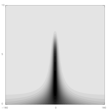
Figure 2: The shade-filled map of the integral( Eq. (20)) as a function of two variables: phase $\Psi_{lm}$ along the horizontal axis and $\rho=|S_{lm}|/\sqrt{\langle|W_{lm}|^{2}\rangle}$ along the vertical axis. The intensity of the gray color corresponds to 20 gray layers from 0 to $\pi^{2}$.

For the $s^{W}_{p}$ signal the definition of the combined phases $\Psi^{M}_{lm}$ for each $(lm)$ mode is similar to Eq. (13):

$$\tan\Psi^{M}_{lm}=\frac{|S_{lm}|\sin\Psi_{lm}+|W_{lm}|\sin\Phi^{W}_{lm}}{|S_{lm}|\cos\Psi_{lm}+|W_{lm}|\cos\Phi^{W}_{lm}}$$ (19)

where $S_{lm}$ is the multipole expansion of the combined signal(CMB $\otimes$ BEAM + PIXEL NOISE) at the mode $(lm)$, $\Psi_{lm}$ the corresponding phase, $W_{lm}$ the controlled noise expansion, and $\Phi^{W}_{lm}$ its phase. The analytical expression for the function $\Delta^{2}(lm)$ can be written in the following way

$$\Delta^{2}(lm)=\frac{1}{2\pi}\int_{-\Psi_{lm}}^{2\pi-\Psi_{lm}}\varphi^{2}d\varphi$$ (20)

$$\left\{e^{-\rho^{2}/2}+\frac{\sqrt{\pi}}{2}\rho\cos\varphi\left[1+\Phi\left(\frac{\rho\cos\varphi}{\sqrt{2}}\right)\right]\right\},$$

where

$$\rho=\frac{|S_{lm}|}{\sqrt{\langle|W_{lm}|^{2}\rangle}},$$ (21)

and

$$\Phi(x)=\frac{2}{\sqrt{\pi}}\int^{x}_{0}e^{-t^{2}}dt.$$ (22)

The integral in Eq. (20) has been tabulated as a function of two variables $\Psi_{lm}$ and $\rho$ and the result is presented in Fig. 2. We will use this tabulation for the numerical experiment in the next section. In this section we will obtain simple analytical asymptotics of Eq. (18).

From Eq. (20) one can find the difference

$$\tan\Psi^{M}_{lm}-\tan\Psi_{lm}=\frac{\frac{|W_{lm}|}{|S_{lm}|}\sin(\Phi^{W}_{lm}-\Psi_{lm})}{\left(1+\frac{|W_{lm}|\cos\Phi^{W}_{lm}}{|S_{lm}|\cos\Psi_{lm}}\right)\cos\Psi_{lm}}.$$ (23)

Let us determine the mean–squared value $\Delta^{2}_{\tan}(lm)$ of the difference between $\tan\Psi^{M}_{lm}$ and $\tan\Psi_{lm}$ using Eq. (23)

$$\Delta^{2}_{\tan}(lm)=\frac{1}{2\pi}\int_{0}^{2\pi}d\Phi^{W}_{lm}\left(\tan\Psi^{M}_{lm}-\tan\Psi_{lm}\right)^{2}.$$ (24)

One finds that $\Delta^{2}_{\tan}(lm)\simeq\Delta^{2}(lm)/\cos^{4}\Psi_{lm}$  if $\Delta^{2}(lm)\ll 1$ and after integration we obtain

$$\Delta^{2}_{\tan}(lm) = \frac{2\alpha_{lm}^{2}(1+\alpha_{lm}^{2})}{(1-\alpha_{lm}^{2})^{3}\cos^{2}\Psi_{lm}}$$ (25)

$$\times\left[1-\frac{\alpha_{lm}^{2}(3-\alpha_{lm}^{2})}{1+\alpha_{lm}^{2}}\cos 2\Psi_{lm}\right]$$

where $\alpha_{lm}=(1-\sqrt{1-\beta_{lm}^{2}})/\beta_{lm}$, and

$$\beta_{lm}=\frac{\sqrt{\langle|W_{lm}|^{2}\rangle}}{|S_{lm}|}\cos\Psi_{lm}\leq\frac{1}{2}.$$ (26)

In the asymptotic $|\beta_{lm}|\ll 1$ we have $\alpha_{lm}=\frac{1}{2}\beta_{lm}\ll 1$ and from Eq. (24) and Eq. (25) we get

$$\Delta^{2}(lm)\simeq\frac{{\langle|W_{lm}|^{2}\rangle}}{2|S_{lm}|^{2}}\left[1-\frac{3{\langle|W_{lm}|^{2}\rangle}}{4|S_{lm}|^{2}\cos^{2}\Psi_{lm}}\cos 2\Psi_{lm}\right].$$ (27)

For our approximation we can neglect the second term in the brackets of Eq. (27) and

$$\Delta^{2}(lm)\approx\frac{{\langle|W_{lm}|^{2}\rangle}}{2|S_{lm}|^{2}}.$$ (28)

Properties of ${\langle|W_{lm}|^{2}\rangle}$ are the same for any values of $l$ (and $m$). Properties of $1/2|S_{lm}|^{2}$ were discussed in the previous section when we discussed $\Delta^{2}_{s}(lm)$. It is obvious that qualitatively the behaviors of the function $\Delta^{2}(lm)$ are the same as $\Delta^{2}_{s}(lm)$. But there is one principal difference between the qualitative and the full correct description of the asymptotic $|S_{lm}|^{2}\rightarrow 0$. Namely, if $|S_{lm}|^{2}\rightarrow 0$ then ${\langle|W_{lm}|^{2}\rangle}/|S_{lm}|^{2}\gg 1$, and the asymptotic Eq. (27) is not valid. Under the condition $|W_{lm}|^{2}\gg|S_{lm}|^{2}$ we have $\Psi^{M}_{lm}\simeq\Phi^{W}_{lm}$ and from Eq. (18) and Eq. (19) we reach

$$\Delta^{2}(lm)\simeq\frac{4\pi^{2}}{3}-\pi\Psi_{lm}+\Psi^{2}_{lm}.$$ (29)

In fact the controlled white noise is some kind of averaging factor in our phase analysis. An analogous method may be used for the power spectrum analysis of the beam asymmetry.

5 The flat sky approximation and numerical results

The general properties of $|S_{lm}|^{2}$ allow us to introduce more convenient and faster flat sky analysis, which is specifically useful for the antenna beam shape estimation. This model reflects the scanning strategy at present specified for the planck mission, when, for a small part of the sky far from the North and South poles, the model of the stable and fixed beam orientation is adequate, without rotation and multi-crossing scans. The implementation of FFT significantly decreases the computational cost, which, for time consuming spherical harmonic analysis, is a major issue.

Using definitions of the signals and noises from the previous section, we define $S_{sky}({\bf k})$ to be the Fourier component of the signal from the sky measured by antenna and $N({\bf k})$ that of the noise, which does not depend on the beam properties. The Fourier modulus and phases of the combined signal are defined as follows,

$$S({\bf k})=S_{sky}({\bf k})+N({\bf k})=\sqrt{C({\bf k})}\exp[i\Phi({\bf k})].$$ (30)

The function $C({\bf k})$ is the power spectrum of the combined signal (observational data and noise) and $\Phi({\bf k})$ describes the phases. $S_{sky}({\bf k})$ represents the CMB signal convolved with the beam. If the signal from the sky does not contain non-Gaussian foreground components (or its manifestation is suppressed at the “cosmologically clean” channels from 70 to 217 GHz (Mandolesi et al. (2000))) and if the noise $N({\bf k})$ is uncorrelated white noise, the distribution of the phases $\Phi({\bf k})$ for different ${\bf k}$ must be random and uniform. If there are some contaminations from the foregrounds and(or) pixel noise is of non-Gaussian nature, the phase distribution over the ${\bf k}$ range can be weakly correlated, and can be tested by phase diagram method(Coles and Chiang (2000)). Such kind of uncertainties of the statistical properties of the signal $C({\bf k})$ are important for separation of the pure CMB signal and noise for complicated characters of the beam shape.

We start out with a squared Gaussian random map with the power spectrum from the angular power spectrum of the $\Lambda$CDM model from Lee et al. (2001). The map simulates a $25.6^{\circ}\times 25.6^{\circ}$ square realization of the CMB temperature fluctuations with pixel size 3 arcmin and periodic boundary conditions (PBC) (see Bond and Efstathiou (1987) and remarks in Section 6). We then add pixel noise, $\sigma_{noise}\sim 6\times 10^{-6}$, after convolving the map with an elliptical beam with long-axis and short-axis FWHM 12 and 9 arcmin, respectively. After generation of the map, which models the HFI 100 GHz frequency channel, we sum $M=10^{2}$ realizations of the controlled noise with variance $W^{2}$ close to the pixel noise variance (Eq. (17) and $W^{2}\sim\langle N^{2}({\bf k})\rangle$) and calculate the mean squared difference between phase of the signal and that of the signal plus controlled noise in the flat sky approximation:

$$\Delta^{2}({\bf k})=\langle\left[\Psi_{n}({\bf k})-\Psi({\bf k})\right]^{2}\rangle|_{M}.$$ (31)

Analogously we can calculate $\Delta_{s}(k)$ for the flat approximation. In Fig. 1 we display the function $\Delta_{s}(k)$, it is rather difficult, however, to draw the averaged contour lines for $\Delta_{s}(k)$ directly from this map. It is easier to do this for the map of the $\Delta(k)$ function. Fig. 3 displays the $\Delta({\bf k})$ function using color representation of phases (Coles and Chiang (2000)). In the color representation, phases are mapped onto the color circle, so that the phase of each mode is represented by a color hue. Color red represents $0^{\circ}$ and the primary hues are $120^{\circ}$ apart, i.e., phases of $120^{\circ}$ and $240^{\circ}$ are represented by color green and blue. Cyan and other complementary colors magenta and yellow represents $180^{\circ}$ and $300^{\circ}$, and $60^{\circ}$, respectively. For presentation effect, we add the symmetric part (Fourier ring) in the Fourier domain. It is clear from the color map of Fig. 3 that in the center for large-scale modes( small ${\bf k}$), the values of $\Delta({\bf k})$ are approaching zero, shown by color red. This is due to the fact that the phases of large-scale modes( the inner rings) are not “perturbed” by added noise. On small-scale modes( the outer rings), where the phases are dominated by pixel noise, the added controlled noise randomizes the resulting phases when the controlled noise level is chosen the same as that of pixel noise.

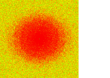
Figure 3: The colored phase map for the $\Delta({\bf k})$ function. The $x$ and $y$ axis are $k_{x}$ and $k_{y}$ axis, respectively. For presentation reason, we show the symmetric part( Fourier ring) in the Fourier domain. The size of the phase map is ranged from $-{\bf k}$ to ${\bf k}$ ( $|{\bf k}|=128$), where $2\pi|{\bf k}|^{-1}\sim$ 12 arcmin.

Figure 4: The contour map of $\Delta_{sm}({\bf k})$ for $k_{s}=7$. The contour level is in unit of degree. The size of the phase map is taken from $-{\bf k}$ to ${\bf k}$( $|{\bf k}|=128$), where $2\pi|{\bf k}|^{-1}\sim$ 12 arcmin.

In the intermediate regime, the beam shape manifests itself through the $\Delta({\bf k})$ function. The fuzzy regions in the intermediate regime reflect the anisotropy of the beam shape. By taking average as

$$\Delta_{sm}({\bf k})=\frac{1}{(2k_{s}+1)^{2}}\sum_{{\bf k}^{{}^{\prime}}\in S}\Delta({\bf k}^{{}^{\prime}}),$$ (32)

where $S=\{{\bf k^{{}^{\prime}}}:\{|k_{x}-k_{x}^{{}^{\prime}}|<k_{s}$, $|k_{y}-k_{y}^{{}^{\prime}}|<k_{s}\}\}$, we can find the mean shape of the beam. Figure 4 shows the contour map of the $\Delta_{sm}({\bf k})$ function by $k_{s}=7$. From the contour map, the elliptic shape is estimated roughly to have the same ratio of the simulated beam shape, i.e., 4/3.

An important issue is related to the asymmetric beam extraction from a real map, covering a small patch of the sky. Previously we used periodic boundary condition (PBC) for modeling the CMB signal (Bond and Efstathiou (1987)). In reality, for some square $\Theta\times\Theta$ patch of the whole sky map, the PBC is artificial and one can ask how sensitive this controlled noise method is to the deviation of the artificial phases of the signal from the true distribution? To answer this question we show in Fig. 5 the result of a numerical experiment for a map which was constructed in the following way: We generate, as described earlier, the PBC map with the size $\Theta_{p}\times\Theta_{p}$, $\Theta_{p}=25.6^{\circ}$, and extracted from this map the inner part $\Theta_{np}\times\Theta_{np}$ with the size $\Theta_{np}=12.8^{\circ}$. We then apply the controlled noise method for the non-PBC map and compare our results of the beam extraction with the PBC case. Figure 5 shows the colored map of this $\Delta$ function. In order to compare with the PBC case, only half of $k$-range of interest is extracted from non-PBC case, as the beam size relative to the map is now twice of the PBC case. The peculiarity of the red crossing is induced by the non-PBC. The difference between these two models is less then $5{\%}$. This implies that we can apply our method for small real patch of the sky directly.

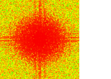
Figure 5: The colored phase map of $\Delta$ function for non-PBC map, which is extracted from the central part of the previous $25.6^{\circ}\times 25.6^{\circ}$ PBC simulated map. The $x$ and $y$ axis are $k_{x}$ and $k_{y}$ axis, respectively. To compare with Fig. 3, we only show half of the $k$-range of Fig. 3, i.e., from $-{\bf k}$ to ${\bf k}$( $|{\bf k}|=64$), where $2\pi|{\bf k}|^{-1}\sim$ 12 arcmin.

6 Conclusion

In this paper we propose the method of power and phase analysis to demonstrate the manifestation of the anisotropy of the antenna beam shape incorporated in the pixelized CMB anisotropy data, and how to estimate the shape of the beam.

It is worth noting that the numerical realization of the phase diagram method described above is based on the flat sky approximation and illustrates the general properties of the CMB signal extraction from the pixelized sky map at the high multipole limit $l\gg 1$. In such a case, the Fourier analysis reflects directly the general properties of the phases of a signal on the sphere, which in the general (whole sky) limit must be defined using spherical harmonic analysis. But there are a few balloon experiments (boomerang, maxima, tophat) which cover relatively small areas of the sky in comparison with planck and the recently launched map missions. Moreover, for the beam shape extraction from map and planck missions it will be convenient to extract preliminary information about antenna beam shape without time consuming spherical harmonic computations. In connection with the planck mission this approach looks promising due to otherwise high computation cost in the framework of the $C(l)$ extraction program.

As it is shown, the functions $\Delta^{2}_{s}({\bf k})$ and $\Delta^{2}({\bf k})$ reflect the general properties of the power spectrum ${C({\bf k})}$ measured from the small patch of the sky.

At the end of this discussion we would like to give the following remark. For estimation of the asymmetry of the antenna beam shape using the controlled noise method, we need to know the limit of the beam cross-level (in dB), for which we can extract the peculiarities of the beam. According to general prediction of the beam shape properties for the planck mission it is realistic to assume that the ellipticity of the beam preserves up to the cross-level $\nu\simeq-10$ dB. For a small patch of the map we can use $B({\bf k})\sim\exp\left[-k^{2}_{x}/(2\sigma^{2}_{+})-k^{2}_{y}/(2\sigma^{2}_{-})\right]$ and $C({\bf k})$ for the best fit $\Lambda$CDM cosmological model from the MAXIMA-1 data. Because of logarithmic dependence of the beam shape parameters on the $C({\bf k})$ and $\sigma^{2}_{N}$:

$$\frac{k^{2}_{x}}{2\sigma^{2}_{+}}+\frac{k^{2}_{y}}{2\sigma^{2}_{-}}\simeq-\ln\left[\frac{C({\bf k})}{\sigma^{2}_{N}}\right]$$

we can find the ratio $\sigma^{2}_{-}/\sigma^{2}_{+}$ with 3-5 $\%$ accuracy at the cross-level $\nu\simeq-6$ dB. This method is most applicable to the patch of sky at low declination where the assumption of stable orientation of the antenna beam is satisfied. A more general case will be investigated in a separate paper.

References

- Bond and Efstathiou (1987) Bond, J.R., & Efstathiou, G. 1987, MNRAS, 226, 655
- Burigana et al. (1998) Burigana, C., et al. 1998, A&AS, 130, 551.
- Coles and Chiang (2000) Coles, P., & Chiang, L.-Y. 2000, Nature, 406, 376
- Hobson and Lasenby, (1998) Hobson, M.P., & Lasenby, A.N. 1998, MNRAS,298,905.
- Lee et al. (2001) Lee, A.T., et al., preprint(astro-ph/0104459).
- Maino et al. (1999) Maino, D., et al. 1999, A&AS, 140, 1
- Mandolesi et al. (2000) Mandolesi, N. et al. 2000, A&AS 145, 323
- Naselsky et al. 2000 (a) Naselsky, P., Novikov D., & Silk J., preprint(astro-ph/0001733)
- Naselsky et al. 2000 (b) Naselsky, P., Novikov, D., Novikov, I., & Silk, J., preprint (astro-ph/0012319).
- Tegmark (1996) Tegmark, M. 1996, ApJ, 470, 81
- Wu et al. (2001) Wu, J.H.P. et al. 2001, ApJS, 132, 1