Automated optical identification of a large complete northern hemisphere sample of flat spectrum radio sources with $S_{\rm 6cm}>200$ mJy

Abstract

This paper describes the automated optical APM identification of radio sources from the Jodrell Bank - VLA Astrometric Survey (JVAS), as used for the search for distant radio-loud quasars. Since JVAS was not intended to be complete, a new complete sample, JVAS++, has been constructed with selection criteria similar to those of JVAS ($S_{5GHz}>200$ mJy, $\alpha_{1.4-5GHz}>-0.5$), and with the use of the more accurate GB6 and NVSS surveys. Comparison between this sample and JVAS indicates that the completeness and reliability of the JVAS survey are $\sim 90\%$ and $\sim 70\%$ respectively. The complete sample has been used to investigate possible relations between optical and radio properties of flat spectrum radio sources. From the 915 sources in the sample, 756 have an optical APM identification at a red ($e$) and/or blue ($o$) plate, resulting in an identification fraction of 83% with a completeness and reliability of 98% and 99% respectively. About $20$% are optically identified with extended APM objects on the red plates, e.g. galaxies. However the distinction between galaxies and quasars can not be done properly near the magnitude limit of the POSS-I plates. The identification fraction appears to decrease from $>$90% for sources with a 5 GHz flux density of $>1Jy$, to $<$80% for sources at 0.2 Jy. The identification fraction, in particular that for unresolved quasars, is found to be lower for sources with steeper radio spectra. In agreement with previous studies, we find that the quasars at low radio flux density levels also tend to have fainter optical magnitudes, although there is a large spread. In addition, objects with a steep radio-to-optical spectral index are found to be mainly highly polarised quasars, supporting the idea that in these objects the polarised synchrotron component is more prominent. It is shown that the large spread in radio-to-optical spectral index is possibly caused by source to source variations in the Doppler boosting of the synchrotron component.

1 Introduction

Over the last decade, a comprehensive catalogue of compact flat spectrum radio sources, the Jodrell Bank $-$ VLA Astrometric Survey (JVAS), has been constructed (Patnaik et al, 1992; Browne et al., 1997; Wilkinson et al., 1998). The main aim of this survey was to provide the astronomical community with a network of bright radio sources with accurate positions ($\sim 10-15$ mas) primarily intended for use as phase calibrators for the Jodrell Bank MERLIN, the VLA and VLBI networks. In addition to its astrometric goals, JVAS proved an effective means of finding radio sources exhibiting strong gravitational lensing, with six systems confirmed to date (King et al. 1999).

Its virtually complete northern-sky coverage makes JVAS uniquely suited for studying the high luminosity end of the flat spectrum radio source population. Our group has been particularly involved in the search for distant quasars (Hook et al. 1996, Hook et al. 1998, Hook & McMahon 1998). As part of this project, sources in the JVAS survey were optically identified using the catalogue output of the APM (the Automated Plate Measurement Facility at Cambridge) scans of the POSS-I plates. This catalogue is ideal for identifying large samples of objects, since they are generated in an automated way allowing an objective assessment of their reliability and homogeneity.

This paper describes the automated optical identification procedure of JVAS, as used for the search for distant quasars. It can be used as a guidance for future projects, involving the optical identification of comprehensive samples of flat spectrum radio sources, like those in the Cosmic Lens All Sky Survey (CLASS; Myers et al. 2001). Since JVAS is not complete, a new sample is constructed using selection criteria similar to those of JVAS, but with the emphasis on completeness, and with the use of more accurate selection surveys. By comparing this sample with JVAS, the completeness of JVAS is assessed. This is described in section 2. Section 3 and 4 describe the APM-POSS-I catalogue and the optical identification procedure of JVAS and its complete counterpart. Section 5 gives the results and discusses possible relations between optical and radio properties using the complete sample.

2 A complete sample of flat spectrum radio sources

2.1 The Jodrell Bank $-$ VLA Astrometric Survey (JVAS)

The JVAS catalogue has been presented in three separate papers, for the regions $+35^{\circ}\leq\delta\leq+75^{\circ}$ (Patnaik et al., 1992), $+0^{\circ}\leq\delta\leq+20^{\circ}$ (Browne et al., 1997), and $+20^{\circ}\leq\delta\leq+35^{\circ}$ and $+75^{\circ}\leq\delta\leq+90^{\circ}$ (Wilkinson et al., 1998). Their initial source list was constructed using the Greenbank surveys conducted at 1.4 and 5 GHz by Condon & Broderick (1985, 1986) and Condon, Broderick & Seielstad (1989), selecting all sources with spectral indices larger than $\alpha=-0.5$ ($\alpha$ defined as $S_{\nu}\propto\nu^{\alpha}$) and $S_{5GHz}\geq 200$ mJy, excluding the region $|b|<2^{\circ}.5$. The 5 GHz flux densities used to construct the sample were determined directly from the maps and have been found to be systematically higher by $\sim 10\%$ than the flux densities determined by Gregory and Condon (87GB, 1991) from the same maps. Since the main goal of JVAS was to construct a grid of phase calibrator sources, and the distribution of the sample above contained some undesirable large holes ($\sim 5^{\circ}$) in some areas, a few additional sources were selected with $S_{5GHz}\geq 150$ mJy to fill these holes. Where possible, the potential calibrator sources were cross-checked against lower frequency surveys to make sure they had genuine flat spectra. The resulting source list was observed with the VLA at 8.4 GHz between 1990 and 1992 (Patnaik et al, 1992; Browne et al., 1997; Wilkinson et al., 1998). The resulting catalogue includes sources with observed 8.4 GHz peak brightness $\geq 50$ mJy/beam.

For sources that are in the regions $+0^{\circ}\leq\delta\leq+20^{\circ}$ and $+35^{\circ}\leq\delta\leq+75^{\circ}$ the rms position error was estimated to be approximately 10 mas in each coordinate (Patnaik et al., 1992; Browne et al., 1997). For sources in the regions $+20^{\circ}\leq\delta\leq+35^{\circ}$ and $+75^{\circ}\leq\delta\leq+90^{\circ}$ this was estimated to approximately be 40 mas (Wilkinson et al., 1998). The resulting catalogue contains 2121 radio sources.

2.2 The selection of a complete flat spectrum sample

Survey	Freq.	Wave-	Reso-	Flux	Position
		length	lution	Density	Error
	(GHz)	(cm)	(arcsec)	(mJy)	(arcsec)
87GB	4.85	6.2	210	$>$25	10$-$30
GB6	4.85	6.2	210	$>$18	10$-$30
GB1400	1.40	21.4	710	$>$150	30$-$70
NVSS	1.40	21.4	45	$>$2.5	1$-$7

Table 1: The relevant parameters of the radio surveys used for the selection of JVAS and JVAS++.

The JVAS catalogue was primarily intended to provide phase calibrators with a uniform sky distribution, and was not intended as a statistically complete flat spectrum sample. Therefore, a similar, complete sample has to be defined to be able to conduct statistically meaningful optical/radio studies. This sample, which we call JVAS++, will then also be used to assess the completeness of JVAS.

The JVAS++ sample was constructed using similar selection criteria as used for the Cosmic Lens All Sky Survey (CLASS; Myers et al. 2001), and is based on the recently available and more accurate radio surveys, the GB6 at 5 GHz (Gregory et al. 1996), and the NVSS at 1.4 GHz (Condon et al. 1998). All the relevant parameters of the radio surveys involved are given in table 1. In the selection procedure, the 1.4 GHz flux density of a GB6 radio source is defined as all the NVSS flux within 70^′′ of the GB6 position (as used for CLASS). The sample has the following selection criteria:

• GB6 5 GHz flux density, $S_{5GHz}>200$ mJy

• declination, $0^{\circ}<\delta<75^{\circ}$, galactic latitude, $|b|>30^{\circ}$.

• radio spectral index, $\alpha_{1.4-5GHz}>-0.5$.

In this way, 915 sources were selected. The distribution on the sky is shown in figure 1. The high galactic latitude cut-off was chosen to reduce the possible influence of galactic foreground extinction. Furthermore, the APM catalogue is only available at these latitudes. About 16% (153) sources are not in the JVAS sample and have been observed with the VLA in B configuration at 8.4 GHz as part of the CLASS survey, in a similar manner as the targets in the JVAS sample (Myers et al. 2001). These provided us with radio positions at an accuracy similar to those of the JVAS sources. Fifty-eight sources are fitted by multiple components at 8.4 GHz. For these, the positions of the brightest components are used. Fifteen objects are not detected with the VLA, all exhibiting extended structure on arcminute scales.

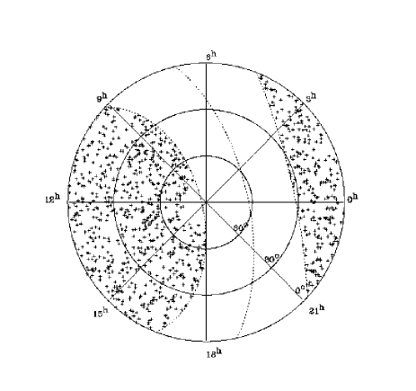
Figure 1: Polar projection of the sky distribution of the sources in the complete sample. The dotted lines indicate the $0^{\circ}$ and $\pm 30^{\circ}$ galactic latitudes.

2.3 The completeness and reliability of JVAS

JVAS contains 762 sources which overlap with JVAS++. In the same area of sky, another 371 sources are part of JVAS, but are not in JVAS++. In addition, 153 objects are in JVAS++, but are not part of JVAS.

The large differences between the JVAS and JVAS++ are due to several effects:

• the use of different selection surveys for JVAS.

• the use of a difference flux density scale for JVAS, which was found to be offset by 10% at 5 GHz.

• the use of a variety of spectral data in the target selection, the non-detection of some sources, and the exclusion of some sources for which the observed VLA position was found to be offsetted by more than 40 arcseconds from the pointing position.

Figure 2: The completeness and reliability of the JVAS survey as function of GB6 5 GHz flux density (left) and 1.4-5 GHz Spectral index (right), with respect to JVAS++ as defined in section 2.

Figure 3: The distribution of the normalised differences in 1.4 GHz flux density of the GB1400 and NVSS catalogues for all the sources in the complete sample, (left), steep spectrum sources (middle) and flat spectrum sources (right).

Figure 4: The distribution of the normalised differences in 5 GHz flux density of the GB6 and 87GB catalogs for all the sources in JVAS++, (left), only the steep spectrum sources (middle), and only the flat spectrum sources (right)

The use of a different flux density scale at 5 GHz, implies that the actual selection criteria for JVAS are, $S_{5GHz}>180$ mJy, and $\alpha_{1.4-5}>-0.58$. This effect, in combination with the inclusion of sources with 150 mJy $<S_{5GHz}<$ 180 mJy, to fill holes in the sky distribution, causes the low reliability of JVAS. Note that since these sources are fainter than 200 mJy, they do not influence the reliability above this flux density, which is typically $>95\%$ (see fig. 2, left). However, they are included, when the reliability is plotted as function of spectral index (fig. 2, right), causing it to be typically $<75\%$.

The use of different selection surveys has three effects. Firstly, the Greenbank 1400 MHz survey, used for the selection of JVAS, has a 12^′ FWHM resolution, compared to 45^′′ for the NVSS and a search radius of 70^′′ used for the revised ‘complete’ sample. Therefore, sources with extended structure at arcminute scales may have been excluded from JVAS with $\alpha<-0.5$, but included in the comparison sample. This is reflected in Figure 2 (left), showing that the completeness of JVAS is decreasing to $\sim 50\%$ at the steep spectral index cut-off. Indeed 49 objects exhibit extended structure at arcminute scales. These are shown in the appendix, where their NVSS images are overlaid with data from the Digitized Sky Survey (Lasker et al. 1990).

Secondly, the use of different selection surveys may cause sources to be included or excluded due to their possible intrinsic variability. Thirdly, measurement uncertainties may cause differences in the selection. To show the influences of variability and measurement uncertainties on the selection process, the Greenbank 1400 MHz observations were compared with the NVSS, and the 87GB data were compared with the GB6. Figure 3 shows the normalised differences between the GB1400 and NVSS flux densities for the sources in the complete sample, with no radio spectral selection on the left, ‘steep’ spectrum ($\alpha<-0.2$) sources in the middle, and ‘flat’ spectrum ($\alpha>-0.2$) sources in the right panel. About 12% of the sources do not have a GB1400 flux density since they are too faint to be in the catalog by White & Becker (1992). These are excluded from the analysis. The NVSS flux densities were decreased by 3% to match the GB1400 flux density scale. The distributions are overlaid by Gaussians with $\sigma=$ 0.13, 0.13, and 0.25 respectively. The distribution for the flat spectrum sources is clearly much broader ($\sigma=0.25$) than that for steep spectrum objects ($\sigma\sim$ 0.13). This indicates that the differences between GB1400 and the NVSS for flat spectrum sources is dominated by variability, which is about 2 times larger than the measurement uncertainties. From a similar distribution of normalised flux density differences between NVSS and the FIRST survey (White et al. 1997), we found that the measurements errors in both FIRST and NVSS are about 5%. This means that, assuming that the distribution of the steep spectrum sources is solely due to measurement errors, the GB1400 survey has an uncertainty in flux density of 12%. Note that this uncertainty has a proportional term and a constant term, the latter due to noise and confusion. In FIRST and NVSS, this constant term is unimportant for our sample. However for the GB1400 survey with a noise level of $\sim 25$ mJy, this factor probably dominates the uncertainty in flux density for the faintest sources.

A similar analysis has been carried out for the two selection surveys at 5 GHz, which is shown in figure 4. The GB6 and 87GB are not independent; GB6 is based half of on the 87GB dataset, and half on a similar dataset, taken a year earlier. Since we are interested in the variability aspect, we assumed that the flux densities of the sources in the second dataset is $2\times GB6-87GB$. The normalised differences between the flux densities taken at these epochs are shown in figure 4, with on the left with no spectral selection, in the middle for steep spectrum sources, and at the right for flat spectrum sources. The distributions are overlaid with a Gaussian with a $\sigma$ of 0.14, 0.14, and 0.17 respectively. Assuming that the distribution of the steep spectrum sources is solely due to measurement uncertainties, each dataset has a typical error of 10%, and the uncertainty in flux density of the GB6 is 7%. The constant noise term of GB6 is expected to contribute for only 2% for the faintest sources in the sample. Note that the flat spectrum sources seem to be only slightly variable, compared to the data at 1.4 GHz, although flat spectrum sources are known to be increasingly variable towards higher frequencies. This is due to the fact that the time-baseline at 5 GHz ($\sim$ 1 year) is much shorter than at 1.4 GHz ($\sim$ 10 years).

It is difficult to estimate the completeness and reliability of JVAS and JVAS++, due to all the effects described above. Most of the differences between the two samples are not caused by incompleteness or unreliability of JVAS, but due to a difference in selection criteria. To assess the completeness of JVAS and JVAS++, we performed a simple simulation. We treated the NVSS and GB6 data as infinitely accurate and added Gaussian distributed offsets (with $\sigma$’s as estimated above) to the flux densities, and determined how many sources enter and leave the sample. In this way, the completeness and reliability of JVAS++ were estimated both to be 95% respectively. For JVAS, we changed the selection criteria to $\alpha_{1.4-5GHz}>-0.58$ and $S_{5GHz}>180$ mJy after the offsets were added, to mimic the use of a different flux density scale. In addition it was assumed that all the sources with $S<160$ mJy were added artificially in JVAS to fill in holes in the sky distribution ($\sim$100 objects). In this way the completeness and reliability of JVAS was estimated to be 90% and 70% respectively.

3 The automated optical identification procedure

3.1 The APM $-$ POSS-I catalogue

Optical identification of sources in the JVAS and JVAS++ samples was carried out using the output catalogue of the APM scans of the Palomar Sky Survey (POSS-I) photographic plates in the $e$ (red) and $o$ (blue) passbands (Bunclark & Irwin, 1983). Plates were scanned with $\sim 0.5^{\prime\prime}$ pixels. The APM covers the Northern sky with $|b|\geq 20^{\circ}-30^{\circ}$. For each detected object a magnitude was measured and the image classified for the $e$ and $o$ plates separately. The images were classified as galaxies, stellar, merged objects or noise based on combinations of various image parameters such as moments, ellipticities etc. The spread in the distribution of each parameter with respect to the stellar locus was used to weight that parameter when combined to form a final classification parameter. The distribution of the combined parameter has a mean and spread which is dependent on magnitude, and a statistical correction was calculated to convert these for the stellar objects to Gaussian distributions with zero mean and rms=1. This correction was then applied to all images and the standard deviation from a stellar profile $N\sigma_{c}$ was recorded. For images about 2 magnitude above the plate limit, this classification is $\sim 90\%$ accurate.

The $e$ and $o$ catalogues were merged, assuming that sources within 2^′′ are one and the same object. Objects with centroids on the $e$ and $o$ plates which differ in position between 2 and 4^′′ were considered to be “nearly” matches. In such case only the position on the E plate were preserved. The final positions of the objects were corrected for subtle distortions of the plates which are most prominent near the plate edges.

The zero-point for photometry in each field was calculated by assuming that the $e$ plate has a limiting magnitude of 20.0 and by assuming a universal, magnitude independent position in the colour-magnitude plane for the stellar locus, as described by McMahon & Irwin 1992. The zero-point of the magnitude system has an rms accuracy of 0.3 magnitude.

The APM $-$ POSS-I catalogue can be accessed via the internet at www.ast.cam.ac.uk/$\sim$apmcat.

3.2 The optical-radio correlation

Three source lists were constructed:

• Sources which are part of both JVAS++ and the JVAS sample (762 objects)

• Sources which are only part of JVAS++ (153 objects)

• Sources which are only part of JVAS (371 objects)

Hence, the combination of sources in lists I and II make up JVAS++, and the sources in lists I and III make up the JVAS sample (in the selected area of sky). The three lists were correlated with the APM$-$POSS-I catalogue, selecting all optical objects within $30^{\prime\prime}$ of each 8.4 GHz radio position. For the objects with extended radio structure at arcminute scales, the radio-optical overlays, as shown in the appendix, were used to search for a possible bright optical identification. These were added manually. The distributions of $\Delta\alpha_{opt-rad}$ and $\Delta\delta_{opt-rad}$ are shown in figure 5, for sources in the JVAS++ sample, excluding objects which exhibit multiple components at 8.4 GHz and/or extended structure at arcminute scales. From these plots the accuracy of the APM positions was determined, by fitting the $\Delta\alpha$ and $\Delta\delta$ distributions with a Gaussian on top of a flat distribution, as expected for a combined population of genuine identifications and random background objects. It shows that the APM positions have an uncertainty of rms=0.4^′′ in both $\alpha$ and $\delta$, and show no systematic offsets to the radio positions.

Figure 5: The distribution of $\Delta\alpha_{opt}-\alpha_{rad}$ and $\Delta\delta_{opt}-\delta_{rad}$, for all the optical objects to a radio position of a JVAS++ source.

Figure 6: The offsets between the JVAS++ positions and the optical APM positions. The solid line indicates a fit to the background source density of 0.0006 arcsec^-2.

Figure 6 shows the distribution of sources around the JVAS++ positions. The solid line is a fit to the background source density of 0.0006 arcsec^-2. We found that this background level was not enhanced by possibly related cluster objects around the radio sources, by counting the number of objects within a 30^′′ radius, offset 5^′ north from each source. It is therefore expected that $\sim 2\%$ of the sources have a random background object within 3 arcsec from their radio position. Such a background object will be incorrectly identified as the optical identification unless the genuine identification is detected and has an APM position closer to the radio position.

Unfortunately, for several reasons the errors in the optical positions are not Gaussian distributed, as assumed above:

• Bright galaxy identifications: The central positions of bright extended objects, e.g. nearby galaxies, can be determined significantly less accurate in the APM than those of fainter stellar objects.

• Merged Objects: Due to the limited resolution of the APM scans, two or more nearby sources are sometimes merged into one single object. In such a case, the central position of the merged object can be several arcseconds away from the position of one of the individual objects (i.e. the identification).

• Bright Stars: Bright Stars, can obliterate other objects in their vicinity, or can produce spurious images.

• Anomalies in the APM Catalogue:. In very rare cases the APM can produce nonsensical results unrelated to any of the former effects, e.g. plate defects such as dirt and scratches, aeroplane tracks and asteroids.

These effects produce a broad non-Gaussian tail in the error distribution at a $\sim 5-10\%$ level. To identify these problems for the individual objects, all the APM images were checked by eye and compared with images from the Digital Sky Survey as retrieved from Skyview. In the course of this process the images were also searched for possible surrounding groups or clusters of galaxies. In addition, if no identification in the APM was found, it was checked whether a possibly faint identification was visible in the DSS. All the JVAS and JVAS++ sources which were found to have one of these problems are shown in the appendix.

3.3 Completeness and reliability of the optical identifications

The likelihood method (de Ruiter, Arp and Willis, 1977) was used to quantify the identification procedure. First, for each candidate identification the following dimensionless measure of the uncertainty in position difference, $r$, was calculated:

$$r=\sqrt{\frac{\Delta\alpha^{2}}{\sigma_{\alpha opt}^{2}}+\frac{\Delta\delta^{2}}{\sigma_{\delta opt}^{2}}}$$ (1)

where $\Delta\alpha$ and $\Delta\delta$ are the offsets between the optical and radio positions, and $\sigma_{\alpha opt}$ and $\sigma_{\delta opt}$ the uncertainties in the optical right ascension and declination positions. The error in the radio position is small $<0.05^{\prime\prime}$ compared to the optical error ($0.55^{\prime\prime}$) and therefore neglected. Given the normalised position difference $r$ for a certain radio-optical pair, the likelihood ratio is defined by (de Ruiter, Arp and Willis, 1977)

$$LR(r)=\frac{dp(r|id)}{dp(r|c)}=\frac{r\ e^{\frac{-r^{2}}{2}}}{2\lambda\ r\ e^{-\lambda r^{2}}}=\frac{1}{2\lambda}e^{\frac{r^{2}(2\lambda-1)}{2}}$$ (2)

where $\lambda=\pi\sigma_{\alpha opt}\sigma_{\delta opt}\rho_{bg}=0.5\rho_{bg}$, where $\rho_{bg}$ is the background source density which is stored for each POSS-plate in APM calibration files. This is the ratio of the probability that a given object found between $r$ and $r+dr$ is the correct identification $p(r|id)$, divided by the probability that it is a contaminating object $p(r|c)$. The cumulative distribution of likelihood ratios is shown in figure 7.

Figure 7: The cumulative distribution of likelihood ratios for the complete sample.

The likelihood ratio cutoff used for this sample is 1.0 which means the probability that the given object is the correct identification is at least equal to the probability that it is a background object. Using this cutoff we find an identification rate, $\theta$, of 83% (i.e. 756 out of 915). This identification fraction can be related to the two a posteriori probabilities that the object found at an angular distance $r$ from the radio source position is a genuine identification, $p(id|r)$, or a confusing object, $p(c|r)$, using Bayes’ theorem

$$p(id|r)=\frac{\theta\ LR(r)}{\theta\ LR(r)+1-\theta}\ \ \ \ \ p(c|r)=\frac{1}{\theta\ LR(r)+1-\theta}$$ (3)

It was assumed that the sources which were found to be merged objects or bright galaxies have an infinite likelihood ratio, resulting in $p(id|r)=1$ and $p(c|r)=0$. The likelihood ratios of the objects, for which the manual check has shown they have a genuine optical identification but a large radio-optical position offset, are set to $2\times 10^{3}$, as if the offset was zero, and therefore as 100% reliable identifications. The completeness, $C$, of the identifications, which is the number of accepted identifications over the number of correct id’s, and the reliability, $R$, which is the fraction of identified sources for which the identification is correct, are given by:

$$C=1-\biggl{(}\sum_{L<1}p(id|r)\biggr{)}/N_{id}$$ (4)

$$R=1-\biggl{(}\sum_{L>1}p(c|r)\biggr{)}/N_{id}$$ (5)

where, $N_{id}$ is the total number of identifications. These correspond to a completeness $C=99\%$ and a reliability $R=99\%$ for LR$\geq 1$ used.

4 Results and discussion

Three tables were produced for the three source lists, which are shown in the appendix, with a detailed description of the columns.

4.1 Radio spectral properties and optical identifications

The JVAS++ sample is uniquely suited to study the high luminosity end of the flat spectrum radio source population. Figure 8 shows the $e$-magnitudes of the optical identifications as function of their $o-e$ colours, classified as stellar (filled circles) and extended (open circles) objects on the red plates. Objects with only limits on the colours are not shown. The colours of the extended objects are more biased towards the red than those of the stellar identifications, as expected for quasars and galaxies, which are found to have generally blue and red optical colours respectively, This can also be seen in figure 9 where the colour-distribution of the two classes of objects are shown. Only at $e>19$, near the plate limit, does this picture get blurred, since no reliable classification can be made and the large majority of objects are classified as stellar.

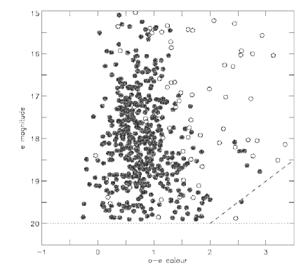
Figure 8: The red $e$ magnitude as function of $o-e$ colour for extended (open circles) and stellar (filled circles) identifications. The dotted and dashed lines indicate the limit in $e$ magnitude and the average limit in $o$ magnitude (which differs per plate) respectively.

Figure 9: The normalised $o-e$ colour distribution for the JVAS++ identifications. The dashed and dotted lines represent the stellar and the extended objects respectively.

Figure 10 shows the optical identification fraction as function of GB6 flux density. The upper line indicates the total identification fraction (including extended, stellar and merged objects). The middle line indicates the fraction of JVAS++ sources identified with APM objects classified as stellar in the red band. The lower line indicates the fraction of JVAS sources identified with APM objects classified as extended in the red band. There is a hint that both the total and stellar identification fraction decrease with decreasing flux density. These two effects are likely caused by a change-over to galaxy identifications at faint flux density levels, which leads to more loss against the plate limit. A similar effect at a similar flux density level has been seen by Shaver et al. (1997) and Falco, Kochanek & Muñoz (1998). Note that due to the uncertain classification near the plate limit, the true decrease in identification fraction for quasars with flux density may even be more pronounced.

Figure 10: The fraction of JVAS++ sources identified with APM objects (total), APM objects classified as stellar and classified as extended in the red band, as function of GB6 flux density. The uncertanties for the total sample are similar to those for the stellar objects.

Figure 11 shows the optical identification fraction as function of 5.0 to 1.4 GHz spectral index. The lines indicate the specific identification fractions as in figure 10. Clearly, the total and stellar identification fractions decrease towards steeper spectral indices, while the fraction of sources identified with extended objects appears to be independent of spectral index. This trend can be explained by assuming that at $\alpha<-0.3$, the unbeamed population of ‘steep’ spectrum galaxies contributes significantly to the total radio source population. Most of these radio galaxies will be too faint to appear on the POSS, and will be unidentified radio sources. This results in a drop in the total identification fraction and the identification fraction of quasars.

Figure 11: The fraction of JVAS++ sources identified with APM objects (total), APM objects classified as stellar and classified as extended in the red band, as function of 8.4-1.4 GHz spectral index.

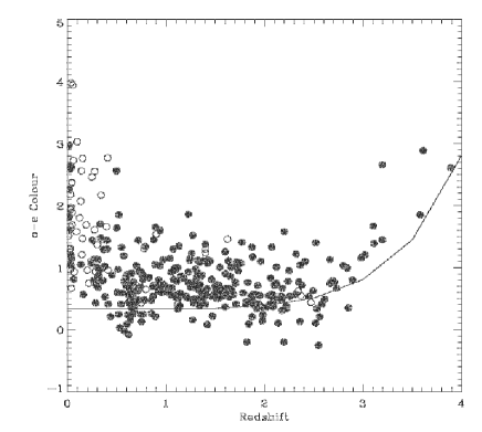
Figure 12: The $o-e$ colour of extended (open circles) and stellar (filled circles) objects as function of redshift, for all sources with an available redshift.The solid line indicates the expected $o-e$ colour of an average quasar reddened by intergalactic absorption (see text).

For the optical identifications with available redshifts in the literature, the $o-e$ colours are shown as function of redshift (figure 12). This figure should be interpreted with great care, since it includes a strong observational bias, e.g. towards bright galaxies and red quasars. Therefore, not surprisingly, most of the extended optical objects (galaxies) are observed to be at $z<0.5$. They are clearly redder than the stellar objects at similar redshifts. Note however that a few objects which are classified as extended, are found at much larger redshifts. Their optical spectra show that they are actually quasars, wrongly classified as extended objects in the APM. There is a clear trend that the optical colours of the quasars become redder towards high redshifts. This is a well known effect and the forms the basis of the colour selection of candidate high redshift quasars (Hook et al. 1996), and is due to intervening Ly$\alpha$ absorption systems. Note however, that the majority of the objects in this redshift regime was actually selected for spectroscopic follow up on the basis of their red colour ($o-e\geq 1.0$), which may have strengthen this effect. The solid line indicates the expected $o-e$ colour of an average quasar reddened by intergalactic absorption. As a quasar spectrum, a power law with spectral index of $-$0.5 was used with emission lines taken from the composite quasar spectrum as constructed by Francis et al. (1991). For the intergalactic absorption the model of Madau (1995) was used. The model follows the trend of redder colours towards high redshift well. At low redshift the data are systematically redder than the model. This is probably due to a contribution of underlying galaxy light.

It is interesting to investigate the relation between the optical apparent magnitude of a quasar and its radio flux density, since both should be related to the power output of the central engine. Bolton & Wall (1970) showed that objects at fainter flux densities tend to have fainter optical magnitudes, but that there is a large spread. This trend is also present in figure 13 (left), where the e-magnitude is shown as function of 5 GHz flux density for sources which are classified as stellar on the red plates, and which have a blue $o-e<1.0$ colour. This can also be seen in figure 14, where for the same subsample, the magnitude distributions are shown for bright (GB6$>$1 Jy), intermediate (350 mJy $>$ GB6 $>$1 Jy), and faint (GB6 $<$ 350 mJy) radio sources.

Figure 13: (left) The $e$ magnitude versus of 5.0 GHz flux density for radio sources identified with blue $o-e<1.0$ stellar objects. (right) The $e$ magnitude versus of 5.0 GHz flux density for radio sources in the sample, which have optical polarisation measurements in the literature, with ’L’ and ’H’ denoting low and high polarisation quasars. Objects at $z<0.5$ have been omitted. The dotted line indicates an optical-to-radio spectral index of $-$0.75.

Figure 14: The magnitude distributions for bright (GB6$>$1 Jy), intermediate (350 mJy $>$ GB6 $>$1 Jy), and faint (GB6 $<$ 350 mJy) radio sources, optically identified with blue $o-e<1.0$ stellar objects.

It is interesting to investigate what may cause this large spread in the ratio of optical to radio luminosity. We noticed that many of the optically faintest quasars were known to be High Polarised Quasars (HPQ); objects which exhibit optical polarisation at levels $>3\%$. In the right panel of figure 13 the $e$ magnitude versus 5 GHz flux density is shown for objects in the sample which have their optical polarisation properties studied by Fugmann & Meisenheimer (1988) or Wills et al. (1992). Indeed, it shows that the HPQ (’H’) prefer to have high radio to optical flux ratios while the low polarised quasars (LPQ; ’L’) show low ratios. Objects at $z<0.5$ were excluded from this plot, to avoid possible host galaxy contamination, and to exclude the population of nearby BL Lac objects and optically violent variable (OVV) quasars which also show high optical polarisation, but often combined with low or rapidly varying radio to optical flux density ratios.

The distribution of HPQs and LPQs is consistent with the idea that the optical quasar light is a combination of a polarised synchrotron component plus an unpolarised component (e.g. Smith et al. 1994). If the unpolarised component is significantly brighter than the synchrotron component (LPQ), then the radio flux (also synchrotron) will be relatively faint compared to the optical, resulting in a ‘flat’ optical to radio spectral index. If the unpolarised component is fainter (HPQ), and a constant spectral index is assumed for the synchrotron component, then the radio flux will be relatively bright, resulting in an overall ‘steep’ radio-to-optical spectral index. Indeed, the dashed line in figure 13 (right) indicates an optical-to-radio spectral index of $-$0.75, with most of the LPQs and HPQs situated above and below this line respectively.

The most straightforward explanation of why the ratio of the polarised to unpolarised components varies so much from quasar to quasar is Doppler boosting of the synchrotron component (eg. Wills et al. 1992). We therefore hypothesise that the large spread in optical to radio luminosity ratios is caused by source to source variations of Doppler boosting of the radio flux, leaving the unpolarised component of the optical emission unaffected. The fact that in our sample we see the HPQs fainter than the LPQs is counter-intuitive since these are the boosted objects. However, in this scheme, the HPQs are not the boosted counterparts of the LPQs in the sample, but are the boosted counterparts of a population which is fainter in the optical and radio. If this explanation is correct, then a correlation is expected between the Doppler factor and the optical to radio spectral index. Lähteenmäki & Valtaoja (1999) estimated the Doppler factors of eighty of the brightest flat spectrum objects in the sky, using total flux density variation monitoring data at 22 and 37 GHz. Thirty-nine objects in their sample overlap with JVAS. Nineteen of those are located at $z>0.5$, and have APM identifications with $o-e<1.0$ (to avoid possible influence of the host galaxy and extinction). For the optical and radio flux densities, the average of $o$ and $e$ magnitudes, and the average of 1.4, 5.0 and 8.4 GHz flux densities are used, to minimise the influence of variability. The estimated Doppler boosting, $D_{var}^{3}$, is plotted against the optical-to-radio spectral index in figure 15. It shows that the Doppler factor is indeed correlated (97% significance) with the radio-to-optical spectral index, and that the slope of the relation is as expected as for the hypothesis that the large spread in optical to radio luminosity ratios is caused by source to source variations of Doppler boosting of the radio flux leaving most of the optical emission unaffected. Evidently, this scheme is too simplistic. First of all, the spectral index of the synchrotron component is most likely steeper in the optical than in the radio, causing the boosting to be stronger in the optical than in the radio, changing the observed optical-to-radio spectral index of the synchrotron component. Furthermore, in the optical we may see a related, but younger part of the synchrotron component, which possibly exhibits different boosting properties, complicating the simple picture scetched above.

Figure 15: The Doppler boosting, estimated by Lähteenmäki & Valtaoja (1999) as function of radio to optical spectral index, for bright JVAS sources. The line indicates the expected relation if the change in spectral index is due to Doppler boosting of only the radio emission, leaving the optical unaffected.

However, the main idea is supported by two previous studies. Firstly, Yee & Oke (1978) and Shuder (1981) showed that the emission line luminosity for a range of AGN types is proportional to the luminosity of the underlying optical continuum over four orders of magnitude. Secondly, Rawlings & Saunders (1991) found that the emission line luminosity of an unbiased sample of FRII radio galaxies is approximately proportional to the total jet kinetic power, which is closely coupled to the power of the central engine. This implies that the optical luminosity should also be a direct indicator of the jet power, hardly affected by Doppler boosting. Indeed, Wills & Brotherton (1995) use the ratio of the radio core to optical continuum luminosity, $R_{V}$, which is the equivalent to the radio-optical spectral index as used in this paper, as an improved measure of quasar orientation over the ratio of radio-core to lobe flux density, $R$. They show that the use of $R_{V}$, rather than $R$, results in a significantly improved inverse correlations with the beaming angle as deduced from apparent superluminal velocities and inverse-Compton-scattered X-ray emission, and with the FWHM of a quasar’s broad H$\beta$ emission line. The use of optical continuum luminosity rather than extended radio luminosity to represent the unbeamed jet power probably works better because the latter is more affected by source-to-source differences in the intergalactic medium (Wills & Brotherton, 1995), and source age.

5 Summary

We have described the automated optical identification procedure of the sources from the Jodrell Bank $-$ VLA Astrometric Survey (JVAS), and a similar, complete radio sample, JVAS++, using the APM scans of the POSS-I plates. It yields an identification rate of 83%, with a completeness and reliability of both 99%. About 20% is identified with extended objects, eg. galaxies. The identification rate appears to drop towards lower flux densities, and towards steeper radio spectra, especially for the stellar classifications. Furthermore, the optical fluxes of quasars with faint radio flux densities appear to be biased towards fainter magnitudes, although there is a large spread in the optical-to-radio spectral index. It is shown that this large spread in radio-to-optical spectral index may be caused by source to source variations in the Doppler boosting of the synchrotron emission.

Appendix A

Tables 2,3, 4 show the optical-radio catalogue for the source lists I, II, and III, as defined in section 2. For each table, column 1 gives the name (JVS=JVAS, CLS=CLASS), columns 2 the radio position (J2000), columns 3, 4, and 5 give the optical-radio offset in right ascension, declination and in total. Column 6 gives the logarithm of the likelihood ratio. Columns 7 to 12 give the APM magnitude, classification (-1=stellar, 1=extended, 2=merged) and psf for the red and blue plate respectively. Column 13 gives the APM colour, columns 14, to 17 give the radio flux densities at 5 GHz (GB6), 1.4 GHz (NVSS and GB1400), and at 8.4 GHz (JVAS). Column 18 gives the redshift as found in the NASA/IPAC Extragalactic Database (NED). Column 19 gives a possible comment. The comments are explained in table 4. The optical parameters are not shown if $\Delta\alpha,\Delta\delta>3.0^{\prime\prime}$, unless the check by eye has shown that a larger optical-radio position offset is the result of a bright galaxy or a merged object identification, or due to extended radio emission.

Figure 17 show all the sources for which the APM did not give a good representation. The three panels show $4^{\prime}\times 4^{\prime}$ representations of the Digitized Sky Survey, The APM-red, and the APM blue data. The number in the left corner indicates the optical-radio position offset.

Figure 16 shows contour plots of NVSS data of objects in the complete sample showing extended structure on arcminute scale. The greyscales represent optical Digitized Sky Survey data. Image sizes are 12’. The dashed circle indicate a 70” radius around the GB6 position.

Figure 16 (gif) to go here

Figure 16: Extended radio sources in the complete sample.

Figure 17 (gif) to go here

Figure 17: All the JVAS sources with anomalies in the APM data.

table 2 can be found at www.roe.ac.uk/ ignas

Table 2:

table 3 can be found at www.roe.ac.uk/ ignas

Table 3:

table 4 can be found at www.roe.ac.uk/ ignas

Table 4:

Table 5: Explanation of the comments in tables 2, 3, and 4.

Code	Comment
a	Blended Object
b	Bright Galaxy
c	Possible ID on DSS?
d	Group/Cluster?
e	Bright Star nearby
f	ID not Possible
g	wrong representation in APM
h	Possible Blended Object?
i	ID is Correct
j	Offset in Red Plate
k	Blended Object in Blue
l	Blended Object in Red
m	Red and Blue APM are shifted
n	Bright Galaxy Nearby
o	DSS not Uniform
p	NVSS extended
q	NVSS several components
r	NVSS Wide angle tail
s	NVSS Double
t	NVSS triple
u	Radio Source is Lobe

References

- [1] Bolton J.G. & Wall J.V., 1970, Australian J. Phys., 23, 789
- [2] Browne I.W.A., Patnaik A.R., Wilkinson P.N., Wrobel J.M., 1998, Monthly Notices of the R.A.S., 293, 257
- [3] Condon J.J., and Broderick J., 1985, Astron. J., 90, 2450
- [4] Condon J.J., Broderick J.J., & Seielstad G.A. 1989, the Astronomical Journal, 97 1064
- [5] Condon, J.J., Cotton, W.D.,Greisen, E.W., Yin, Q.F., Perley, R.A., Taylor, G.B., Broderick, J.J., 1998, the Astronomical Journal, 115, 1693
- [6] Gregory P.C. and Condon J.J., 1991, Astrophys. J. Suppl., 75, 1011
- [7] Gregory P.C., Scott W.K., Douglas K., Condon J.J., 1996, Astrophys. J. Suppl., 103, 427
- [8] Falco E.E., Kochanek C.S., Muñoz J.A., 1998, the Astrophysical Journal, 494. 47
- [9] Francis, P.J., Hewett, P.C, Foltz C.B., Chaffee, F.H., Weymann, R.J., Morris S.L., 1991, the Astrophysical Journal, 373, 465
- [10] Fugmann W., Meisenheimer K., 1988, A&A Suppl., 76, 145
- [11] Hook, I.M., McMahon, R.G., Irwin, M.J., Hazard, C., 1996 Monthly Notices of the R.A.S., 282, 1274
- [12] Hook I.M., Becker R.H., McMahon R.G., White R.L., 1998, Monthly Notices of the R.A.S. 297, 1115
- [13] Hook I.M., McMahon, 1998, Monthly Notices of the R.A.S. 294, L7
- [14] King L.J., Browne I.W.A., Marlow D.R., Patnaik A.R., Wilkinson P.N., 1999, Monthly Notices of the R.A.S., 307, 225
- [15] Lähteenmäki A., Valtaoja E., 1999, the Astrophysical Journal, 521, 493
- [16] Lasker, B.M., Sturch C.R., McLean B.J., Russell, J.L., Jenkner H., Shara M.M., 1990, Astronomical Journal, 99, 2019
- [17] Madau P., 1995, the Astrophysical Journal, 441, 18
- [18] McMahon, R.G. & Irwin, M.J., 1992, In Digitised Optical Sky Surveys Ed. H.T.MacGillivray & E.B.Thomson, Astrophysics and Space Science Library, 174, 417
- [19] Myers et al, 2001, in preparation
- [20] Patnaik A.R., Browne I.W.A., Wilkinson P.N., Wrobel J.M., 1992, Monthly Notices of the R.A.S., 254, 655
- [21] de Ruiter H.R., Arp H.C., Willis A.G., 1977 Astr. & Astrophys. Suppl., 28, 211
- [22] Shuder, J.M., 1981, ApJ, 244, 12
- [23] Shaver P., Wall J., Kellermann K., Jackson C., Hawkins M., 1997, in ‘The Early Universe with the VLT. ’, eds, Jacqueline Bergeron (Berlin, Springer), p.349
- [24] Smith P.S., Schmidt G.D., Jannuzi B.T., Elston R., 1994, Astrophysical Journal, 426, 535
- [25] Wilkinson P.N., Browne I.W.A., Patnaik A.R., Wrobel J.M., Sorathia B., 1998, Monthly Notices of the R.A.S., 300 790
- [26] White R. L., Becker, R. H., Helfand, D. J., & Gregg, M. D., 1997, Astrophysical Journal, 475, 479
- [27] White, R. L., Becker, R. H., 1992, Astrophysical Journal Suppl., 79, 331
- [28] Wills B.J., Brotherton M.S., 1995, ApJ, 448, L81
- [29] Wills B.J., Wills D., Breger M., Antonucci R.R.J., Barvainis R., 1992, Astrophysical Journal, 398, 454
- [30] Yee H.K.C., Oke J.B., 1978, ApJ, 226, 753