Thermal emission from low-field neutron stars
We present a new grid of LTE model atmospheres for weakly magnetic ( G) neutron stars, using opacity and equation of state data from the OPAL project and employing a fully frequency- and angle-dependent radiation transfer. We discuss the differences from earlier models, including a comparison with a detailed NLTE calculation. We suggest heating of the outer layers of the neutron star atmosphere as an explanation for the featureless X-ray spectra of RX J1856.5–3754 and RX J0720.4–3125 recently observed with Chandra and XMM.
Key Words.:
stars: neutron – stars: atmospheres – radiative transfer – radiation mechanisms: thermal1 Introduction
Modern X-ray observatories detect the thermal surface emission of a number of neutron stars. In analogy to the classic model atmosphere analysis of normal stars, such observations permit the direct measurement of fundamental neutron star properties, such as their effective temperatures, atmospheric abundances and surface gravities. The latter point is especially of great importance, as an accurate measurement of the surface gravity of a neutron star is (with the distance known) equivalent to a measurement of its mass/radius ratio. The observational confirmation/rejection of the predicted neutron star mass-radius relations is a fundamental test of our understanding of the physics of matter above nuclear densities.
The first neutron star model atmospheres involving realistic opacities were computed by Romani (1987, henceforth R87), using atomic data from the Los Alamos Opacity Library and employing a simple angle-averaged radiation transfer. As a major result, R87 could show that the thermal emission of neutron stars differs substantially from a Planck spectrum. For low-metallicity (helium) atmospheres, the emitted spectrum is harder than the corresponding blackbody spectrum. The spectra emitted from high-metallicity atmospheres (carbon, oxygen or iron) are closer to a blackbody distribution, but show strong absorption structures in the energy range observable with X-ray telescopes.
Rajagopal & Romani (1996, henceforth RR96) computed hydrogen, solar abundance, and iron model atmospheres for low-field neutron stars, using improved opacity and equation of state data from the OPAL project (Iglesias & Rogers 1996), but employing the same radiation transfer as R87. Contemporaneously, a similar set of low-field atmospheres, partially based on the same atomic OPAL data, but employing a more sophisticated radiation transfer, was presented by Zavlin et al. (1996, henceforth ZPS96). The RR96 and ZPS96 models, broadly confirming the results of R87, were applied to X-ray observations of presumably low-field neutron stars, i.e. millisecond pulsars (RR96, Zavlin & Pavlov 1998), isolated neutron stars (Pavlov et al. 1996), and transiently accreting neutron stars in quiescent LMXBs (e.g., Rutledge et al. 1999, 2000, 2001).
In the case of strongly magnetic neutron stars ( G), both the observation and the computation of the thermal surface emission is significantly more difficult, as non-thermal magnetospheric radiation dilutes the surface emission and as little atomic data is readily available (for a review of the properties of matter in strong magnetic fields, see Lai 2001). Magnetic models for hydrogen and iron atmospheres were computed by Pavlov et al. (1995) and Rajagopal et al. (1997), respectively.
The wealth of high-quality neutron star observations expected from Chandra and XMM justifies the computation of modern model atmospheres. In this paper, we present new model atmosphere grids for low-field neutron stars that overcome a number of shortcomings and errors in the RR96 and ZPS96 calculations and that are made available to the community.
2 The model atmospheres
The new grid of neutron star atmospheres was computed combining a fully frequency- and angle-dependent radiation transfer code (Gänsicke et al. 1995) and the OPAL opacities from RR96. The employed radiation transfer is part of a model atmosphere code that has previously been used for the computation of white dwarf atmospheres which have been widely applied to observations of cataclysmic variables and white dwarf/main-sequence binary stars.
The model atmospheres were created under the following assumptions. (1) Plane-parallel geometry. The atmosphere of a neutron star has a vertical extension of a few centimeters at most, compared to a radius of km. Its curvature is hence completely negligible. (2) Hydrostatic equilibrium. For the extreme surface gravity of neutron stars and the relatively low temperatures that we consider here, the atmosphere is static. The situation is different in accreting neutron stars during X-ray bursts, where the nuclear burning atmosphere considerably expands on short time scales. (3) Radiative equilibrium. The atmosphere contains no source of energy, but acts only as a blanket, through which the thermal energy of the underlying core leaks out. In Sect. 3, we will discuss how abandoning this assumption will impact the spectrum of the neutron star. (4) Local thermal equilibrium (LTE). For the high densities and the low temperatures in the considered atmospheres collisional ion-ion interactions dominate over interactions between matter and the radiation field throughout most of the atmosphere. Deviations from LTE in the outermost tenuous layers of the atmosphere may somewhat affect the depth of the absorption lines, but considering the overall level of uncertainty in the atomic physics involved, and the relatively poor quality of the available spectroscopy, the assumption of LTE appears to be a reasonable approximation. Below, we discuss a quantitative comparison to a NLTE model.
With these approximations, the computation of a model atmosphere can be separated into two independent parts: calculating the structure of the atmosphere from the integration of the hydrostatic equation (Sect. 2.1) and solving the radiation transfer (Sect. 2.2). The temperature structure of the atmosphere, , is a free parameter in the overall process and is adjusted iteratively until radiative and hydrostatic equilibrium are satisfied (Sect. 2.3).
2.1 Atmosphere structure
The vertical scale of the atmosphere is transformed from the geometrical depth to the optical depth by , with the total mean opacity (see below) and the density. The structure of the atmosphere is then obtained by integrating the equation of hydrostatic equilibrium
| (1) |
where is the gas pressure, from an outer boundary to an inner boundary . Considering the extremely high surface gravity encountered in a neutron star atmosphere, we neglect the effects of radiation pressure. We compute a starting value for the integration of eq. (1), , assuming that the outer layers of the atmosphere are isothermal and that the degree of ionization is constant. With ,
| (2) |
being itself a function of , we use as an estimate and solve eq. (2) with a Newton-Raphson method. From we proceed with the integration of eq. (1) to .
This integration involves at each depth the evaluation of the equation of state (EOS) as well as the computation of the absorption and scattering coefficients. For the EOS and the radiative opacities, we use the OPAL data (Iglesias & Rogers 1996) from RR96, that cover three different chemical compositions: hydrogen, solar abundances, and iron. The opacities are tabulated as a function of the temperature , with the temperature in K, and , with the photon energy (for additional details on the OPAL opacity tables, see RR96). For a given depth in the atmosphere, defining and and at a given energy, the radiative absorption coefficient is calculated from the opacity tables using a bilinear interpolation in and and a linear interpolation in . In the construction of the model atmospheres, the radiative absorption coefficient for a finite energy interval is given by the harmonic mean of individual evaluations of , with within , and sufficiently large to sample well the resolution of the OPAL tables. Thomson scattering is an important source of opacity only in low-Z atmospheres at high temperatures and high energies. The OPAL tables implicitly include Thomson scattering as radiative opacity. is, hence, the sum of true absorption plus Thomson scattering. We will come back to this issue in Sect. 2.2. Finally, we compute a radiative Rosseland mean opacity from the energy dependent .
Following RR96, we include a conductive opacity (Cox & Giuli 1968) to account for energy transport by electron conduction, with the number of electrons per a.m.u., the average atomic mass, the average ionic charge, and the temperature in K. The radiative (Rosseland) opacity and the conductive opacity are harmonically added. The total opacity is, hence, given by .
Once eq. (1) is integrated to , a complete macroscopic description of the atmosphere structure is at hand.
2.2 Radiation transfer
For the assumption given above, the radiation transfer equation takes the form
| (3) |
with the cosine of the angle between the normal to the atmosphere and the direction of the considered radiation beam, the frequency-dependent optical depth, the frequency- and angle-dependent specific intensity, and the source function.
As mentioned in Sect. 2.1, Thomson scattering is implicitely included in the OPAL opacity tables. Considering that the contribution of Thomson scattering to the total opacity is negligible in high-Z atmospheres, we restrict an explicit treatment of Thomson scattering to our hydrogen models (Sect. 2). We compute Thomson scattering, , but taking into account the cross-section reduction by collective effects (Boercker 1987), with the electron density in , calculated under the assumption of full ionisazion, and the true frequency-dependent absorption , where is the radiative frequency-dependent OPAL opacity from Sect. 2.2.
With the isotropic and, to first order approximation, coherent Thomson scattering term, the source function is given by
| (4) |
with the Planck function and the mean intensity. We use as boundary conditions for eq. (3) at and the diffusion approximation at . Equation (3) is solved using the well-documented Rybicki method (e.g. Mihalas 1978).
For the high-Z composition atmospheres (solar abundances and iron), we treat Thomson scattering as true absorption, directly using the OPAL .
From the resulting angle-dependent specific intensities, the flux at the surface of the atmosphere is computed,
| (5) |
Radiative and conductive equilibrium requires
| (6) |
at each depth in the atmosphere, where is the Stefan-Boltzmann constant, is the conductive energy flux, as detailed in RR96, and is the effective temperature of the neutron star. If the deviations from the equilibrium (6) are larger than a given error, correction terms are computed from linearization of the angle-integrated form of eq. (3) (e.g. Feautrier 1964; Auer & Mihalas 1969, 1970; Gustafsson 1971).
2.3 Model atmosphere computation
The actual computation of a model atmosphere and the emergent spectrum is done in two separate stages.
(i) Starting from the temperature structure of a grey atmosphere (Chandrasekhar 1944), we iteratively construct (Sect. 2.1 and Sect. 2.2) an atmosphere structure that satisfies radiative and hydrostatic equilibrium. At this stage, we use an energy grid of 1000 logarithmic equidistant bins covering the range keV. For each energy bin, 30 evaluations of the OPAL opacity tables are harmonically added for the computation of the radiative absorption coefficient. The atmosphere structure is constructed on an optical depth grid with 100 points covering (except for the coldest models, which were computed on a grid covering due to limitations in the available OPAL data). The angular dependency of the radiation field is sampled by three Gaussian points in . Radiative equilibrium (eq. 6 is satisfied to better then at each optical depth) is reached after iterations. Generally, the hydrogen atmospheres converged the slowest, as the steep drop of the opacity makes the atmosphere transparent for high-energy photons, thus radiatively coupling the deep hot layers with the surface layers. Electron conduction carries a few percent of the total flux at the largest optical depths (Rosseland optical depths ) in the coldest iron and solar atmospheres. For , the conductive flux is less than 1%, which is in good agreement with the estimates of ZPS96. Including the conductive opacity in our atmosphere models has, hence, no noticeable effect on the emergent spectra.
(ii) From a given atmosphere structure, we recompute the emergent spectrum solving the radiation transfer (Sect 2.2) on a much finer energy grid (10 000 bins, 10 OPAL evaluations per bin), and using 6 Gaussian points in to resolve the angular dependence of the specific intensity. The higher number of angular points has practically no influence on the angle-averaged flux from the neutron star surface, but may be used to account for limb darkening in the computation of spectra from neutron stars with non-homogeneous temperature distributions.

2.4 The model spectra
We computed grids of model atmospheres for the three different compositions covered by the OPAL opacity/EOS tables of RR96: hydrogen, solar abundances, and iron. We restricted ourselves to the canonical neutron star configuration, and km, corresponding to a surface gravitational acceleration of . The three grids cover the temperature range in steps of 0.05, i.e. a total of 29 spectra per abundance grid.111The angle-averaged fluxes are available from CDS, for the angle-dependent specific intensities, or models covering additional temperatures/surface gravities, please contact the authors.
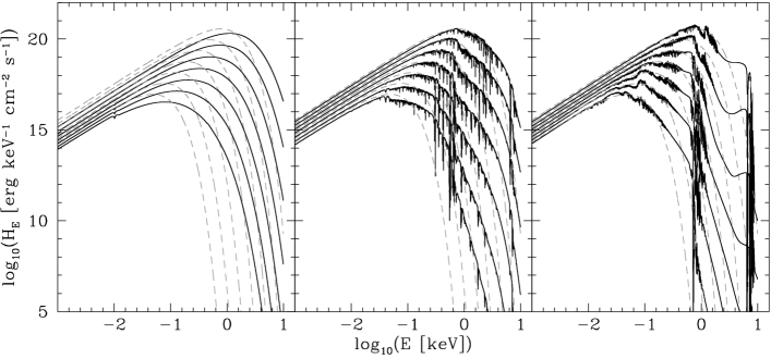
Figure 1 shows the emergent spectra for the three different compositions. As already evident in the previous neutron star atmosphere calculations (R87, RR96, ZPS96), the model spectra differ significantly from blackbody distributions. The pure hydrogen models show a strong flux excess over the blackbody distributions at energies above the peak flux. The free-free and bound-free opacity in these atmospheres drops off rapidly at high energies, leaving Thomson scattering as the dominant interaction between the atmosphere matter and the radiation field. As a consequence, the atmosphere is highly transparent to the hard X-ray photons from deep hot layers. In contrast to the hydrogen models, the iron and solar abundance models are overall closer to the blackbody distributions because of the milder energy dependence of their opacities. They show, however, a substantial amount of absorption structures, lines and edges, which are especially pronounced in the keV range well observable with most of the present and past X-ray satellites.
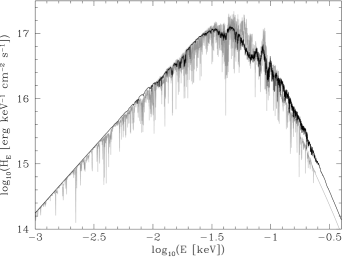
Noticeable absorption structures with equivalent widths of Å are present in the iron spectra of moderately cool neutron stars also in the ultraviolet. The (non-magnetic) hydrogen models contain only the extremely pressure broadened line. In a magnetic field splits in three Zeeman-components, with the components asymmetrically shifted by Å for G (Ruder et al. 1994). Because the hydrogen in these hot atmospheres is ionised to a large extent, the Zeeman components are expected to be rather weak, but they may possibly be detected with future large aperture ultraviolet telecopes, allowing a direct measurement of the magnetic field strength. Figure 2 compares the redshifted222 for an assumed km and . iron and hydrogen spectra in the far ultraviolet.
Figure 3 shows the angle-dependent intensity for a K iron atmosphere. It is apparent that the emission from the neutron star surface is highly anisotropic, as previously discussed by ZPS96. Calculations of the emission of a neutron star with a non-homogeneous surface temperature distribution must take this anisotropy into consideration. An application of the angle-dependent intensities will be discussed elsewhere.

2.5 Comparison to earlier neutron star atmosphere models
2.5.1 Rajagopal & Romani (1996)
The new model spectra agree quite well with the models of RR96. The only systematic differences are found for the hydrogen models, where the new models have a significantly lower flux at energies keV. This difference is due to the inclusion of Thomson scattering in the new models, which increases the opacities at large optical depths in the hydrogen atmospheres. For the heavy element atmospheres, this effect is negligible, as the opacity is dominated by bound-bound and bound-free absorption.
Small (5-15 %) differences in the emergent flux of the heavy element atmospheres are found in the low-temperature () models in the energy range 1–10 keV. The specific intensities at these high energies are orders of magnitude below the peak intensities, and we believe that the differences between the new models and those of RR96 are due to the different numerical treatment of the radiation transfer. At higher energies, the agreement between the two different model generations is better than 1%, except in strong lines where different energy sampling naturally leads to somewhat larger discrepancies.
2.5.2 Zavlin et al. (1996)
ZPS96 computed grids of non-magnetic neutron star LTE model atmospheres for three different compositions, hydrogen, helium, and iron. The hydrogen and helium opacities and non-ideal EOS employed in these models were calculated by ZPS96 using the occupation probability formalism described by Hummer & Mihalas (1988). The iron models were computed using the same OPAL data used also by RR96 and in the present paper. The iron models show a significant difference both in the overall shape of the continuum as well as in the details of the absorption features. We traced this to an erroneous use of the opacity grid in ZPS96. This has been confirmed (Pavlov, priv. comm.)333 After we alerted G. Pavlov to their errors in employing the opacities, their group has computed revised models in reasonable agreement with other work. An example revised spectrum appears in (Pavlov & Zavlin 2000).. The ZPS96 hydrogen model is somewhat harder than both our new spectrum and that of RR96. The flux excess of the ZPS96 model (or the flux deficiency of our model) is not fully understood, but likely stems from small differences in the absorption/scattering opacities.
2.5.3 Werner & Deetjen (2000)
Werner & Deetjen (2000) presented the first NLTE calculation for a neutron star atmosphere using bound-free opacities from the Opacity Project (Seaton et al. 1994) and explicitly treated line blanketing by millions of lines from the Kurucz & Bell (1995) line list. Figure 4 compares the K pure iron NLTE model from Werner & Deetjen (2000) with a corresponding model from our LTE calculations. While the NLTE model clearly shows more detail because of the much larger number of considered transitions, the overall agreement between the two models is very good. Werner & Deetjen (2000) quote a flux difference between their LTE and NLTE models of % in the line cores, and much less in the continuum. For higher temperatures, the NLTE effects might be stronger, but so far no detailed atomic data are available.
3 Beyond “classic” stellar atmospheres
Part of the ongoing effort in computing neutron star atmospheres has been carried out for the analysis of X-ray observations of isolated neutron stars (e.g. Pons et al. 2002). However, recent high-resolution X-ray spectroscopy of the brightest isolated neutron star candidates RX J1856.5–3754 (Burwitz et al. 2001) apparently excludes all the neutron star atmosphere models presented so far: while the overall spectral energy distribution (SED) rules out low- atmospheres, the featureless XMM and Chandra spectra are inconsistent with the strong structures expected from a heavy element atmosphere.
As in all previous calculations (R87, RR96, ZPS96, Werner & Deetjen 2000), the model atmospheres presented here assume radiative equilibrium. It is worth remembering that when the model fits suggest that the flux is dominated by hot polar caps with a small fraction of the full neutron star surface area, some sort of local heating is likely implicated. For instance, anisotropic interior conductivities can produce smooth variations in the surface effective temperture; e.g. Heyl & Hernquist (1998). For slow, long neutron stars, local heating can be caused by low accretion. Zampieri et al. (1995) and Zane et al. (2000) have produced emergent spectra for ionized H stars accreting at low rates. With proton stopping depths of , much of the energy is deposited fairly deep in the atmosphere, but shocks in the accretion flow can apparently heat the outer layers, providing excess flux on the Rayleigh-Jeans tail. For an active magnetosphere, local heating without accretion arises from precipitating (Arons 1981) or from illumination by energetic (polar cap or outer gap) photons.

An analogous situation – pole caps heated by accretion – is well-documented in polars, a subtype of cataclysmic variables in which a strongly magnetic white dwarf accretes from a late type donor star. In theses systems, the white dwarf atmosphere near the magnetic poles is heated by strong irradiation with cyclotron radiation and thermal bremsstrahlung from a stand-off shock. As a consequence of this accretion heating, the spectra of these heated pole caps are almost devoid of spectral structures. The Lyman lines, typically very strong absorption features in the ultraviolet spectra of white dwarfs, are almost completely flattened out (Gänsicke et al. 1998), and also the X-ray spectra of polars are very close to blackbody distributions, unlike the expected emission from a high-gravity photosphere strongly enriched with heavy elements (Mauche 1999). While the physical processes involved in heating the pole caps of accreting white dwarfs and accreting neutron stars differ markedly, the observed phenomenology is very similar: RX J0720.4–3125, another bright isolated neutron star shows a quasi-sinusoidal X-ray light curve suggesting the presence of large heated pole caps, whereas the X-ray spectrum contains no significant absorption structure (Haberl et al. 1997; Paerels et al. 2001) reminiscent of the ultraviolet observations of the heated white dwarf in the polar AM Her (Gänsicke et al. 1998). It appears likely, therefore, that heating effects may affect the line spectra of heavy element neutron star atmospheres.
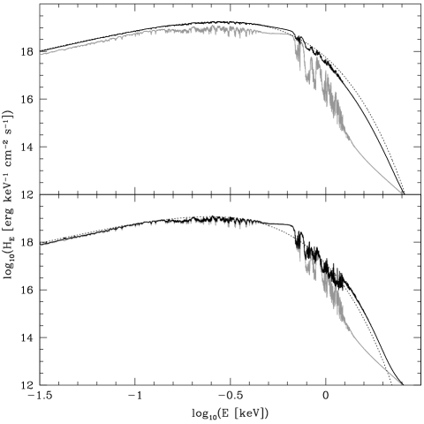
As a simple illustration, we ignored the details of particular physical heating effects and computed a number of spectra under the assumption that an energy is deposited at a characteristic depth in the atmosphere, (Fig. 5). In practice, the emergent spectrum of a “heated” neutron star is computed by (1) modifying the thermal structure of an undisturbed atmosphere to account for the deposited energy, (2) recomputing the atmosphere structure based on the modified temperature profile (Sect. 2.1), and finally solving the radiation tansfer within the “heated” atmosphere (Sect. 2.2). Figure 6 shows the emergent fluxes from a K iron atmosphere for two different sets of parameters, and , equivalent to , and and , equivalent to .
Two effects are evident. The flatter temperature in the outer layers of the heated atmospheres supresses the strong absorption edge around 1 keV, returning the Wien tail colour quite close to that of a simple blackbody. Further, the equivalent widths of the lines are, of course, strongly affected. Heating at strongly supresses the keV absorption features; surface heating in fact drives the line features on the Rayleigh-Jeans tail into emission.
We stress that this illustrative approach is by no means a self-consistent model of a heated neutron star atmosphere, as we include neither any physical assumption on the actual heating mechanims, e.g., there are currently no plausbile physical processes known which are capable of heating such shallow layers, nor a proper energy balance of the heating/cooling processes. It is merely intended as a possible explanation for the apparent paradox that the SEDs of isolated neutron stars (in particular RX J1856.5–3754) are best-fitted with heavy-element model spectra (Pavlov et al. 1996; this paper; Burwitz et al. 2001; Pons et al. 2002), whereas their X-ray spectra show at best very weak spectral structures.
More detailed future work will need to carefully examine the efficiency of the various possible heating mechanisms, in particular to establish the depth-dependent energy deposition, and to account properly for the energy balance in the neutron star atmosphere.
4 Conclusions
We have presented a set of angle-dependant low field neutron star atmosphere spectra. These radiative and hydrostatic equilibrium atmospheres should be useful to researchers pursuing exploratory fits of soft X-ray/UV/optical data. However, it is important to inject a note of caution into the discussion. At a minimum, non-uniform surface temperature, combined with limb-darkening and gravitational focussing will have subtle, but important effects which can be modeled using the present grid.
Many other physical effects can, of course, strongly perturb neutron star spectra. The effects on heavy element absorption lines and edges can be particularly strong. Magnetic fields characteristic of young radio pulsars will have a dramatic effect on the opacities and the emergent spectra. When considering the strength of the absorption lines in spectra from magnetic atmospheres with heavy elements (Rajagopal et al. 1997) it is important to remember that the line energies depend sensitively on the B-field. Even simple dipole variation across a polar cap can shift line energies by %, strongly decreasing the equivalent width of spectral features in phase-averaged spectra. Convection has also been considered (eg. RR96), although even small magnetic fields may supress convective transport and keep atmospheres close to the hydrostatic solution.
On the whole, while we feel that our atmosphere grid should be of use for fitting of observed data; complications are certainly expected. In particular strong -field variations and surface re-heating can decrease the equivalent width of heavy element line features in neutron stars with active magnetosphers; this may explain in part the difficulty in finding such features in early Chandra/XMM data (e.g. Paerels et al. 2001; Burwitz et al. 2001).
Acknowledgements.
BTG was supported in part by a travel grant of the Deutscher Akademischer Auslandsdienst (PKZ: D/99/08935) and by the DLR under grant 50 OR 99 03 6. We thank K. Werner and G. Pavlov for providing their model spectra for a quantitative comparison, and B. Rutledge for comments on an earlier draft. We thank the referee, Dr. Zavlin, for useful comments.References
- Arons (1981) Arons, J. 1981, ApJ, 248, 1099
- Auer & Mihalas (1969) Auer, L. H. & Mihalas, D. 1969, ApJ, 158, 641
- Auer & Mihalas (1970) —. 1970, MNRAS, 149, 65
- Boercker (1987) Boercker, D. B. 1987, ApJ Lett., 316, L95
- Burwitz et al. (2001) Burwitz, V., Zavlin, V. E., Neuhäuser, R., et al. 2001, A&A, 379, L35
- Chandrasekhar (1944) Chandrasekhar, S. 1944, ApJ, 100, 76
- Cox & Giuli (1968) Cox, J. P. & Giuli, R. T., eds. 1968, Stellar Structure, Vol.,I (New Yorl: Gordon & Breach)
- Feautrier (1964) Feautrier, P. 1964, C.R. Acad. Sc. Paris, 258, 3189
- Gänsicke et al. (1995) Gänsicke, B. T., Beuermann, K., & de Martino, D. 1995, A&A, 303, 127
- Gänsicke et al. (1998) Gänsicke, B. T., Hoard, D. W., Beuermann, K., Sion, E. M., & Szkody, P. 1998, A&A, 338, 933
- Gustafsson (1971) Gustafsson, B. 1971, A&A, 10, 187
- Haberl et al. (1997) Haberl, F., Motch, C., Buckley, D., Zickgraf, F.-J., & Pietsch, W. 1997, A&A, 326, 662
- Heyl & Hernquist (1998) Heyl, J. S. & Hernquist, L. 1998, MNRAS, 300, 599
- Hummer & Mihalas (1988) Hummer, D. G. & Mihalas, D. 1988, ApJ, 331, 794
- Iglesias & Rogers (1996) Iglesias, C. A. & Rogers, F. J. 1996, ApJ, 464, 943
- Kurucz & Bell (1995) Kurucz, R. & Bell, B. 1995, Atomic Line Data (R.L. Kurucz and B. Bell) Kurucz CD-ROM No. 23. Cambridge, Mass.: Smithsonian Astrophysical Observatory, 1995., 23
- Lai (2001) Lai, D. 2001, Rev. Mod. Phys., 73, 629
- Mauche (1999) Mauche, C. W. 1999, in Annapolis Workshop on Magnetic Cataclysmic Variables, ed. C. Hellier & K. Mukai (ASP Conf. Ser. 157), 157—168
- Mihalas (1978) Mihalas, D. 1978, Stellar atmospheres, 2nd edn. (San Francisco: W. H. Freeman & Co)
- Paerels et al. (2001) Paerels, F., Mori, K., Motch, C., et al. 2001, A&A, 365, L298
- Pavlov et al. (1995) Pavlov, G. G., Shibanov, Y. A., Zavlin, V. E., & Meyer, R. D. 1995, in The Lives of the Neutron Stars., ed. M. A. Alpar, U. Kiziloglu, & J. van Paradijs (Dordrecht: Kluwer), 71–90
- Pavlov & Zavlin (2000) Pavlov, G. G. & Zavlin, V. E. 2000, in Highly Energetic Physical Processes and Mechanisms for Emission from Astrophysical Plasmas, ed. P. C. H. Martens, S. Tsuruta, & P. Weber (ASP Conf. Ser. 195), 103
- Pavlov et al. (1996) Pavlov, G. G., Zavlin, V. E., Truemper, J., & Neuhaeuser, R. 1996, ApJ Lett., 472, L33
- Pons et al. (2002) Pons, J. A., Walter, F. M., Lattimer, J. M., et al. 2002, ApJ, 564, 981
- Rajagopal & Romani (1996) Rajagopal, M. & Romani, R. W. 1996, ApJ, 461, 327
- Rajagopal et al. (1997) Rajagopal, M., Romani, R. W., & Miller, M. C. 1997, ApJ, 479, 347
- Romani (1987) Romani, R. W. 1987, ApJ, 313, 718
- Ruder et al. (1994) Ruder, H., Wunner, G., Herold, H., & Geyer, F. 1994, Atoms in strong magnetic fields (Heidelberg: Springer)
- Rutledge et al. (1999) Rutledge, R. E., Bildsten, L., Brown, E. F., Pavlov, G. G., & Zavlin, V. E. 1999, ApJ, 514, 945
- Rutledge et al. (2000) —. 2000, ApJ, 529, 985
- Rutledge et al. (2001) —. 2001, ApJ, 551, 921
- Seaton et al. (1994) Seaton, M. J., Yan, Y., Mihalas, D., & Pradhan, A. K. 1994, MNRAS, 266, 805
- Werner & Deetjen (2000) Werner, K. & Deetjen, J. 2000, in Pulsar Astronomy - 2000 and Beyond, ed. M. Kramer, N. Wex, & R. Wielebinski (ASP Conf. Ser. 202), 623–624
- Zampieri et al. (1995) Zampieri, L., Turolla, R., Zane, S., & Treves, A. 1995, ApJ, 439, 849
- Zane et al. (2000) Zane, S., Turolla, R., & Treves, A. 2000, ApJ, 537, 387
- Zavlin et al. (1996) Zavlin, V. E., Pavlov, G., & Shibanov, Y. 1996, A&A, 315, 141
- Zavlin & Pavlov (1998) Zavlin, V. E. & Pavlov, G. G. 1998, A&A, 329, 583