Large scale structures in the Early SDSS:
Comparison of the North and South Galactic strips

Abstract

We compare the large scale galaxy clustering between the North and South SDSS early data release (EDR) and also with the clustering in the APM Galaxy Survey. The three samples are independent and cover an area of 150, 230 and 4300 square degrees respectively. We combine SDSS data in different ways to approach the APM selection. Given the good photometric calibration of the SDSS data and the very good match of its North and South number counts, we combine them in a single sample. The joint clustering is compared with equivalent subsamples in the APM. The final sampling errors are small enough to provide an independent test for some of the results in the APM. We find evidence for an inflection in the shape of the 2-point function in the SDSS which is very similar to what is found in the APM. This feature has been interpreted as evidence for non-linear gravitational growth. By studying higher order correlations, we can also confirm good agreement with the hypothesis of Gaussian initial conditions (and small biasing) for the structure traced by the large scale SDSS galaxy distribution.

1. Introduction

The SDSS collaboration have recently made an early data release (EDR) publicly available. The EDR contains around a million galaxies distributed within a narrow strip of 2.5 degrees across the equator. As the strip crosses the galactic plane, the data is divided into two separate sets in the North and South Galactic caps. The SDSS collaboration has presented a series of analysis (Zehavi etal 2002, Scranton etal 2002, Connolly etal 2002, Dodelson etal 2002, Tegmark etal 2002, Szalay etal 2002) of large scale angular clustering on the North Galactic strip, which contains data with the best seeing conditions in the EDR. Gaztañaga (2001, hereafter Ga01) presented a study of bright ($g^{\prime}\simeq 20$) SDSS galaxies in the South Galactic EDR strip, centering the analysis on the comparison of clustering to the APM Galaxy Survey (Maddox etal 1990).

In this paper we want to compare and combine the bright ($r^{\prime}\simeq 19$ or $g^{\prime}\simeq 20$) galaxies in North and South strips to make a detailed comparison between North and South and also to the APM. Do the North and South strips have similar clustering? How do they compare to previous analyses? What does the EDR tell us about structure formation in the Universe? Answering these questions will help us understanding the SDSS EDR data and, at the same time, will give us the opportunity to test how reliable are conclusions drawn from previous galaxy surveys. In particular regarding the shape of the 2-point function (Maddox etal 1990, Gaztañaga & Juszkiewicz 2001) and higher order correlations (eg Bernardeau et al. 2002, and references therein).

This paper is organized as follows. In section §2 we present the samples used and the galaxy selection and number counts. Section §3 shows the comparison of the 2 and 3-point correlation functions. We end with some discussion and a listing of conclusions.

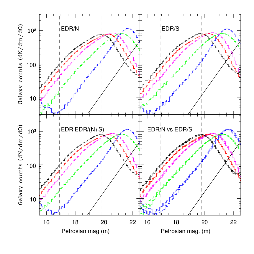
Figure 1.— Galaxy density counts per magnitude bin and square deg. $dN/dm/d\Omega$ as a function of Petrosian magnitude $z^{\prime},i^{\prime},r^{\prime},g^{\prime},u^{\prime}$ (from left to right). The top panels show EDR/N (left) and EDR/S (right). The bottom left panel shows EDR/(N+S) while the right panel compares EDR/S to EDR/N.

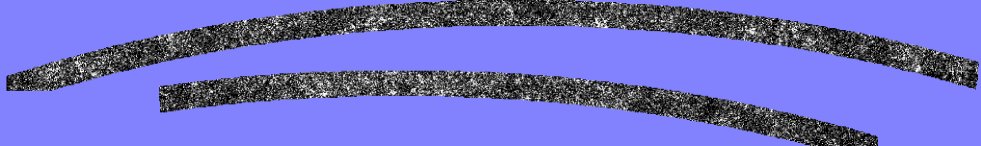
Figure 2.— Pixel maps of equatorial projections of EDR/N (top) with $2.5\times 90$ sqr.deg. and EDR/S (bottom) with $2.5\times 60$ sqr.deg.

2. SDSS samples and pixel maps

We follow the steps described in Gaztañaga (2001, hereafter Ga01). We download data from the SDSS public archives using the SDSS Science Archive Query Tool (sdssQT, http://archive.stsci.edu/sdss/software/). We select objects from an equatorial SGC (South Galactic Cap) strip 2.5 wide ($-1.25<DEC<1.25$ degrees.) and 66 deg. long ($351<RA<56$ deg.), which will be called EDR/S, and also from a similar NGC (North Galactic Cap) 2.5 wide and 91 deg. long ($145<RA<236$ deg.), which will be called EDR/N. These strips (SDSS numbers 82N/82S and 10N/10S) correspond to some of the first runs of the early commissioning data (runs 94/125 and 752/756) and have variable seeing conditions. Runs 752 and 125 are the worst with regions where the seeing fluctuates above 2”. Runs 756 and 94 are better, but still have seeing fluctuations of a few tenths of arc-second within scales of a few degrees. These seeing conditions could introduce large scale gradients because of the corresponding variations in the photometric reduction (eg star-galaxy separation) that could manifest as large scale number density gradients (see Scranton et al 2001 for a detailed account of these effects). We will test our results against the possible effects of seeing variations, by restricting the analysis to runs 756 and 94, and by using a seeing mask (see §3.3).

We will also consider a sample which includes both the North and South strips, this will be called: EDR/(N+S). Note that the clustering from this sample will not necessarily agree with the mean of EDR/N and EDR/S, eg EDR/(N+S) $\neq$ EDR/N+EDR/S (see below).

We first select all galaxies brighter than $u^{\prime}=22.3,g^{\prime}=23.3,r^{\prime}=23.1,i^{\prime}=22.3,z^{\prime}=20.8$, which corresponds to the SDSS limiting magnitudes for 5 sigma detection in point sources (York etal. 2000). Galaxies are found from either the $1\times 1$, $2\times 2$ or $4\times 4$ binned CCD pixels and they are de-blended by the SDSS pipeline (Lupton etal 2001). Only isolated objects, child objects (resulting from deblending) and objects on which the de-blender gave up are used in constructing our galaxy catalog (see Yasuda etal 2001).

There are about 375000 objects in our sample classified as galaxies in the EDR/S and about 504000 in the EDR/N. Figure 1 shows the number counts (surface density) for all these 879000 galaxies as a function of the magnitude in each band, measured by the SDSS modified Petrosian magnitudes $m_{u}^{\prime}$, $m_{g}^{\prime}$, $m_{r}^{\prime}$, $m_{i}^{\prime}$ and $m_{z}^{\prime}$ (see Yasuda et al 2001 for a discussion of the SDSS counts). Continuous diagonal lines show the $10^{0.6m}$ expected for a low redshift homogeneous distribution with no k-correction, no evolution and no-extinction.

We next select galaxies with SDSS modified Petrosian magnitudes to match the APM selection: $17<B_{J}<20$, which corresponds to a mean depth of ${\cal D}\sim 400$ Mpc/h. We try different prescriptions. We first apply the following transformation to mimic the APM filter $B_{J}$:

$$B_{J}=g^{\prime}+0.193(g^{\prime}-r^{\prime})+0.115$$ (1)

This results from combining the relation $B_{J}=B-0.28(B-V)$ (Maddox etal 1990) with expressions (5) and (6) in Yasuda etal (2001). As the mean color $g^{\prime}-r^{\prime}\simeq 0.7$ the above relation gives a mean $B_{J}\simeq g^{\prime}+0.25$, which roughly agrees with the magnitude shift used in Ga01. For the $17<B_{J}<20$ range (using the above transformation) we find $N\simeq 123000$ galaxies in the EDR/(N+S), with a galaxy surface which is very similar to the one in the APM (only $5\%$ larger after substraction of the $5\%$ star-merger contribution in the APM). In any case, this type of color transformations between bands are not accurate and they only work in some average statistical sense. The uncertainties are even larger when we recall that the APM uses fix isophotal aperture, while SDSS is using Petrosian magnitudes, a difference that can introduce additional color terms and surface brightness dependence.

It is much cleaner to use a single SDSS band. We should use $g^{\prime}$ which is the closest to the APM $\lambda_{B_{J}}\simeq 4200A$ ($\lambda_{u^{\prime}}\simeq 3560$, $\lambda_{g^{\prime}}\simeq 4680$ and $\lambda_{r^{\prime}}\simeq 6180$). But how do we decide the range of $g^{\prime}$ to match the APM $17<B_{J}<20$? We try two approaches. One is to look for the magnitude interval that has the same counts, as done in Ga01. The resulting range is $16.8<g^{\prime}<19.8$. This gives a reasonable match to the clustering amplitudes in the EDR/S and EDR/N. But there is no reason to expect a perfect match: the selection function and resulting depth is different for different colors. The other approach is to fix the magnitude range, ie $17<g^{\prime}<20$, rather than the counts. This produces $N\simeq 157000$ galaxies, which corresponds $\simeq 25\%$ higher counts than the APM. This does not necessarily mean that this sample is deeper than the APM, because of the intrinsic different in color selection, K-corrections and possible color evolution.

Finally, we produce equal area projection pixel maps of various resolutions similar to those made in Ga01. Except for a few tests, all the analyses presented here correspond to 3’.5 resolution pixels. On making the pixel maps we mask out about 1.’75 of the EDR sample from the edges, which makes an integer number of pixels in our equatorial projection. This also avoids potential problem of the galaxy photometry on the edges (although higher resolution maps show very similar results, indicating that this is not really a problem).

2.1. Galactic extinction

The above discussion ignored Galactic extinction. It should be noted that the standard extinction law $A_{b}=C(\csc b-1)$ with $C=0.1$ was used for the APM photometry. This is a very small correction: $A_{b}=0$ at the poles ($b=90$ deg) and the maximum $A_{b}\simeq 0.03$ at the lowest galactic declination ($b\simeq 50$ deg). This is in contrast to the Schlegel etal (1998) extinction maps which have significant differential extinction $E(B-V)\simeq 0.02-0.03$ even at the poles. The corresponding total absorption $A_{b}$ for the $B_{J}$ band according to Table 6 in Schlegel etal (1998) is four times larger: $A_{b}\simeq 0.08-0.12$. This increases up to $A_{b}\simeq 0.2-0.3$ at galactic declination $b\simeq 50$. Thus, using the Schlegel etal (1998) extinction correction has a large impact in the number counts for a fix magnitude range. The change can be roughly accounted for by shifting the mean magnitude ranges by the mean extinction, eg $\simeq 0.2$ magnitudes in $B_{J}$. It is therefore important to know what extinction correction has been applied when comparing different surveys or magnitude bands.

Despite the possible impact on the quoted magnitudes (and therefore counts), extinction has little impact on clustering, at least for $r^{\prime}<21$ (see Scranton etal 2001 and also Tegmark etal 1998). This is fortunate because of the uncertainties involved in making the extinction maps and its calibration. Moreover, the Schlegel etal (1998) extinction map only has a 6’.1 FWHM, which is much larger than the individual galaxies we are interested on. Many dusty regions have filamentary structure (with a fractal pattern) and large fluctuations in extinction from point to point. One would expect similar fluctuations on smaller (galaxy size) scales, which introduces further uncertainties to individual corrections.

Here we decided as default not to correct for extinction, because this will be closer to the APM analysis and makes little effect on clustering at the depths and for the issues that will be explored here. This has been extensively checked for EDR/N by Scraton et al. (2001). We have also check this here in all EDR/N, EDR/S and EDR/(N+S), see §3.3

To avoid confusion with other prescriptions by the SDSS collaboration we will use $z^{\prime},i^{\prime},r^{\prime},g^{\prime},u^{\prime}$ for ’raw’, uncorrected magnitudes, and $z^{*},i^{*},r^{*},g^{*},u^{*}$ for extinction corrected magnitudes. For example, according to Schlegel etal (1998) $r^{\prime}=18$ corresponds roughly to an average extinction corrected $r^{*}\simeq 17.9$ for a mean differential extinction $E(B-V)\simeq 0.03$.

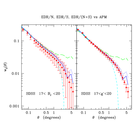
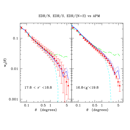
Figure 3.— The angular 2-point function $w_{2}(\theta)$ as a function of galaxy separation $\theta$ for different SDSS magnitudes as labeled in the figures. The short and long dashed lines correspond to the SDSS EDR/N (North) and EDR/S (South) strips. The continuous line corresponds to EDR/(N+S), a joint analysis of the SDSS South and North data. The dotted line is the mean of the EDR/N and EDR/S. The triangles with errorbars show the mean and 1-sigma confidence level in the values of 10 APM sub-samples that simulate the different EDR samples: EDR/S (errors in the first panel), EDR/(N+S) (error in second and fourth panels) and EDR/S (errors in third panel).

3. Clustering comparison

To study sampling and estimation biasing effects on the SDSS clustering estimators we have cut different SDSS-like strips out of the APM map (see Ga01). For the APM, we have considered a $17<B_{J}<20$ magnitude slice in an equal-area projection pixel map with a resolution of $3.5$ arc-min, that covers over $4300$ $deg^{2}$ around the SGC. The APM sample can fit about 25 strips similar to EDR/S and 16 similar to EDR/N. The APM can not cover the combined EDR/(N+S) as it extends across the whole equatorial circle. But we can select several subsamples consisting of sets of 2 strips, one like EDR/S and another one like EDR/N well separated within the APM map, eg by at least $10$ degrees. As correlations are negligible on angular scales $>10$ degrees, this simulates well the combined EDR/(N+S) analysis. To study sampling effects over individual scans we also extract individual SDSS-like CCD scans out of the APM pixel maps. In all cases we correct the clustering in the APM maps for a $5\%$ contamination of randomly merged stars (see Maddox etal 1990), ie we scale fluctuations up by $5\%$ (see also Gaztañaga 1994).

3.1. The angular 2-point function

We first study the angular two-point function. Figure 3 shows the results from the EDR/S (long-dashed), EDR/N (short-dash) and EDR/(N+S) (continuous lines). As mentioned above, the clustering from the combined sample EDR/(N+S) will not necessarily agree with the mean of EDR/N and EDR/S (shown as dotted lines) for several reasons: estimators are not linear, neither are sampling errors and local galaxy fluctuations are estimated around the combined mean density (rather than the mean density in each subsample). As shown in Figure 3 the two estimators yield different results. In general for a well calibrated survey the whole, ie EDR/(N+S), should give better results than the sum of the parts, so that we take the EDR(N+S) results as our best estimate.

In general, the results for the $w_{2}$ shape in EDR/N in Figure 3 agree well with the corresponding comparison in Fig.1 of Connolly etal (2002), with a sharp break to zero around 2-3 degrees. The results for EDR/S agree well with Ga01, showing a flattening at similar scales. Note how EDR/(N+S) $17<B_{J}<20$ (shown in the first panel) are about $15\%$ higher in amplitude that the APM (this is not a very significant discrepancy for the EDR/S errors shown in the plot, but it is when compared to the EDR/(N+S) errors from the APM, shown in panels 2 and 3). As mentioned above this is not totally surprising as the magnitude conversion in Eq.[1] could only works on some average sense. Results for $16.8<g^{\prime}<19.8$ are intermediate between $B_{J}$ and $17<g^{\prime}<20$.

Figure 4.— Pixel maps of the central ($2.5\times 40$ sqr.deg.) region of the EDR/N strip (10N/10S) with the full 752+756 overlapping runs.

Figure 5.— Same as Fig.4 but with only the central part of 6 CCD regions in run 756. With this resolution (3’.5) a CCD field is only a few pixels wide.

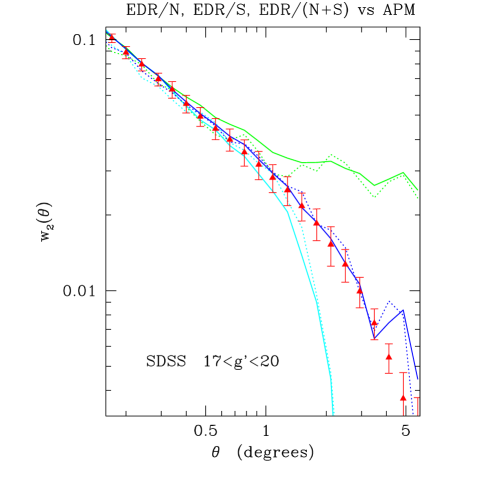
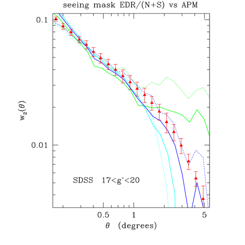
Figure 6.— Left panel: Zoom over a region of the second panel of Figure 3. Here we compare the full strips of EDR/S, EDR/N and EDR/(N+S) (continuous lines from top to bottom at the largest angles) to the APM subsamples (triangle with errorbars) of size similar to EDR/(N+S). The dotted lines correspond to the central part of the CCD in scans 94 (top dotted line, next to EDR/S), 756 (bottom, next to EDR/N) and the joint 756+94 (middle dotted line, along EDR/(N+S)).
 
Right panel: The dotted lines are as in the left panel, while the continuous lines correspond to the seeing mask in Fig.7.

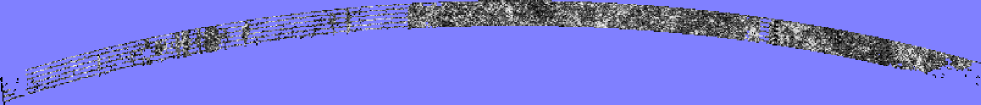
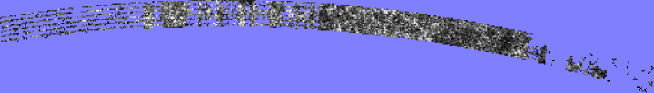
Figure 7.— Pixel maps similar to Fig.2 with the seeing and extinction mask.

Scranton et al 2002 studied the SDSS systematic effects with $r^{*}$ colors, and found that systematic effects had negligible contributions to $w_{2}(\theta)$ for $r^{*}<21$ (eg see their figure 15). The APM has a depth corresponding to $r^{*}\simeq 18.5$, which is almost 3 magnitudes brighter than the above limit. Nevertheless, for comparison, we also study the $w_{2}(\theta)$ shape in $r^{\prime}$. The brighter sample of $r^{*}=18-19$ in Connolly etal (2001) is slightly deeper that the APM, with $z\simeq 0.18$ rather than $z\simeq 0.15$ for the APM. We find that $r^{\prime}=17.8-18.8$ is the closest one magnitude $r^{\prime}$ bin in depth to the APM. Because of the average extinction this corresponds roughly to extinction corrected $r^{*}=17.65-18.65$. This sample has about $40\%$ fewer galaxies (per square degree) than the APM, presumably because of the color correction and differences in the photometric selection. Results for this $r^{\prime}$ sample (shown in the third panel of Figure 3) agree quite well with the APM amplitude. Here the errors are from APM subsamples similar to EDR/N (note how they are slightly smaller than the errors in the APM shown in the first panel of Figure 3, as expected from the smaller area of EDR/S).

Overall, we see how the shape of the 2-point function in all EDR samples remains remarkably similar for the different magnitudes. This is despite the fact that the mean counts change by more than $60\%$ from case to case. The amplitude of $w_{2}$ changes by about $20\%$ from one SDSS sample to the other, but the shape remains quite similar. The best match to the APM amplitude is for the $17<g^{\prime}<20$, which will be taken for now on as our reference sample.

3.2. $w_{2}(\theta)$ in central scans 756 and 94

As a test for systematics, we study $w_{2}(\theta)$ using only the central region of the CCD in scans 756 (North EDR) and 94 (South EDR). The seeing during run 756 is the best in the EDR with only small fluctuations around 1”.4. Regions in the SDSS where the seeing degraded to worse than 1”.5 are marked for re-observations. As this includes most of the EDR data one may worry that some of the results presented here could be affected by these seeing variations . As mentioned above this has been shown not be the case, at least for $r^{*}<21$ (Scranton etal 2001).

We estimate $w_{2}(\theta)$ using only galaxies in the central regions of the CCD in scans 756 (the best of EDR/N) and 94 (the best of EDR/S). Figure 4 shows a piece of this new data set for the EDR/N. As can be seen in the figure (bottom panel) we only consider the central part of 756 to avoid any contamination from the CCD edges. This new data set contains only $30\%$ of the area (and of the galaxies) from the whole strip.

Left panel in Figure 6 compares the results of $w_{2}(\theta)$ for the individual scans against the whole strip for all EDR/S, EDR/N and EDR/(N+S). As can be seem in this Figure, individual scans (dotted lines) agree very well with the corresponding overall strip values. Possible systematic errors seem quite small. In fact, the agreement is striking after a visual comparison of the heavy masking in the pixel maps of Figure 4 (which shows the actual resolution use for the $w_{2}(\theta)$ estimation in Fig. 6). One would naively expect some more significant sampling variations when we use only 1/3 of the data. But nearby regions are strongly correlated and we can get very similar results with only a fraction of the data (this is also nicely shown in Figures 13-15 of Scranton etal 2001). This test shows the power of doing configuration space analysis (as opposed to Fourier space analysis, eg see Scoccimarro etal 2001). It also illustrates that our estimator for $w_{2}(\theta)$ performs very well on dealing with masked data.

3.3. Seeing and reddening mask

Fig.7 shows athe pixels EDR/N and EDR/S with a seeing better than 2 arc-sec. and 0.2 maximum extinction. Pixels with larger seeing or larger extinction are masked out. As apparent in the Figure there is a significant reduction of the available area after the masking. Right panel of Figure 6 compares the results of $w_{2}(\theta)$ for the new masked maps with the results for the individual scans, for all EDR/S, EDR/N and EDR/(N+S). There is now a much better agreement between the EDR/N and EDR/S, which suggest that the discrepancies between EDR/N and EDR/S apparent in the left panel of Fig.7 are due to these systematic effects. The number of available pixels ($30\%$ of the total) is comparable to the ones in individual scans (dotted line), which indicates that samplings errors can not account for the observed differences between the dotted and continuous lines. The biggest change is apparent in EDR/S, which is the smallest sample and the one subject to worst seeing conditions. Most of the difference is due to the seeing rather than the extinction mask.

We find similar results for slightly lower cuts in seeing and extinction, but the number of pixels in EDR/S decrease very quickly as we lower the seeing, and sampling errors dominate over any possible systematics. Thus such a tests are not very conclusive.

Note that the APM absolute errors should be larger for the masked data, as there are less area available. Note also that the mean EDR/(N+S) is lower (continuous middle line in the right panel of Figure 6). The absolute samplings error (as oppose to the relative errors) approach a constant on $\theta\sim 1$ deg. scale (e.g. Fig.8 and Eq.8). All of this indicates that the final relative errors should be larger. Thus, taking into account these considerations, the discrepancies between EDR/N and EDR/S are not significant anymore, and certainly within 2-sigma errors from the APM.

3.4. Variance and covariance

Bernstein (1994) has calculated the covariance in the angular 2-point function $w_{i}\equiv w(\theta_{i})$, where $\theta_{i}$ correspond to the bins in angular separation (for a more general discussion on errors see §6 in Bernardeau et al. 2002). We will consider two main sources of errors. One is due to the finite number of particles ${\cal N}$ in the distribution. This error is usually called the ”Poisson error”, and goes as: $\sim 1/{\cal N}$. The second is due to the finite size of the sample, which is characterized by:

$$w_{\Omega}\equiv{1\over{\Omega^{2}}}\int\int d\Omega_{1}\Omega_{2}~{}w(\theta_{12})$$ (2)

the mean correlation function over the solid angle of the survey $\Omega$. This gives the uncertainty in the mean density on the scale of the sample, which is constrained to be zero in most estimators, as the mean density is calculated from the same sample, i.e. estimators suffer from the integral constraint. In general, this integral is not zero, but we need a clustering model or a larger survey, such as the APM, to calculate its value. For the EDR size, $w_{\Omega}$ is dominated by the value of $w(\theta)$ on the scale of the strip width: $w(\theta=5deg)$. From the APM $w(\theta)$ we find $\simeq 10^{-2}$ for EDR/S. For the APM size itself, this integral should be significantly smaller, but its value is quite uncertain. For both for EDR and APM sub-samples, the Poisson errors $\simeq 1/{\cal N}\simeq 10^{-5}-10^{-6}$ are typically smaller than the sampling errors. Neglecting Poisson errors and using $w_{N}\sim q_{N}~{}w^{N-1}$ for higher order correlations , Bernstein (1994) found:

$$Cov(w_{i},w_{j})\simeq g(\gamma)~{}w_{\Omega}^{2}+\beta~{}w_{\Omega}(w_{i}-w_{\Omega})(w_{j}-w_{\Omega})$$ (3)

where $g(\gamma)$ is a geometric term of order unity for power-law correlations $w(\theta)\simeq A\theta^{\gamma}$. In the strict hierarchical model, $w_{N}=q_{N}~{}w^{N-1}$, we have $\beta=4(1-2q_{3}+q_{4})$. As this model is a rough approximation we will take $\beta$ to be a constant, which will be fitted using the simulations. The corresponding expression for the variance (diagonal of the covariance) is:

$$Var(w_{i})\simeq g(\gamma)~{}w_{\Omega}^{2}+\beta~{}w_{\Omega}(w_{i}-w_{\Omega})^{2}.$$ (4)

In Fig.8 we compare the square root of the above expression $\Delta w(\theta_{i})\equiv\sqrt{Var(w_{i})}$ with the RMS errors in $w_{i}$ from the dispersion in 10 APM sub-samples that simulate the geometry of the EDR/S sample. We find that a value of $\beta\simeq 4$ fits well the above theoretical model to the errors in the simulations. In principle, both $g$ and $\beta$ could be a function of scale, but the model seems to match well the simulations, at least in the range $\theta\simeq 0.1-4.0$ deg. On smaller scales we are approaching the map pixel resolution and we should also include the variance due to the shot-noise and finite cell-size. On scales larger that $\theta\simeq 4deg$ we approach the EDR strip size and the integral constrain becomes important. As we have not corrected for the integral constrain, we do not expect our errors to follow the predictions on large scales. In the intermediate regime the model seems to work quite well.

Bernstein (1994) has shown, using Montecarlo simulations, that the model in Eq.3 works well for the covariance matrix. In his Fig.2 it shows the covariance between adjacent bins $Cov(w_{i},w_{i+1})$. These predictions should work well here if we compare alternative bins $Cov(w_{i},w_{i+2})$ instead of adjacent bins, as we are using 12 bins per decade as opposed to 6 bins per decade in Bernstein (1994). The resulting covariance matrix is close to singular and most of its principal components are degenerate. Thus, a significant test estimation is not just straight forward.

With the help of Montecarlo simulations Bernstein (1994) concluded that the effect of the off diagonal errors is small when fitting parametric models, in particular a power-laws to $w(\theta)$. He find similar results for the amplitude and the slope when using the simple diagonal chi-square minimization or the of the principal components of the full covariance matrix. Both the level of clustering and the errors in his Montecarlo simulations are quite similar to the ones presented here (compare left panel of our Fig.8 to his Fig.1). Thus we can extend the conclusions of Bernstein (1994) to the present analysis and, for simplicity, ignore the off-diagonal errors in the covariance matrix. In order to make sure that the same conditions apply, we should use only every other bin in fitting models.

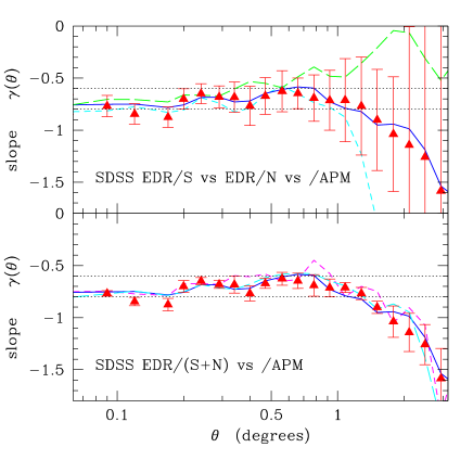
Figure 8.— Left panel: Mean (dotted line) and errors (circles) in $w(\theta)$ from 10 APM sub-samples that simulate EDR/N. The errors are compared with the theoretical expectation in Eq.4 (continuous line). The dashed lines show the contributions from each of the terms in Eq.4.  
Right panel: Logarithmic slope of the angular 2-point function $\gamma(\theta)$ as a function of galaxy separation $\theta$ for SDSS. The lines in the top panel correspond to the ones in the second panel of Fig.3 (ie EDR/S, EDR/N and EDR/(N+S) in $17<g^{\prime}<20$). In the bottom panel we also show the EDR/(N+S) in the corrected $17<B_{J}<20$ (long dashed line), again $17<g^{\prime}<20$ (continuous line) and the central region of the CCDs in scans 756+94 (short dashed line). The triangles with errorbars show the mean and 1-sigma confidence level in the values of several APM sub-samples similar to EDR/(N+S). The errorbars in the top panel corresponds to APM sub-samples similar to EDR/S. The horizontal dotted lines corresponds $\gamma=-0.6$ and $\gamma=-0.8$.

3.5. An inflection point in $w_{2}(\theta)$?

Right panel of Fig.8 shows the logarithmic slope:

$$\gamma(r)={d\log w_{2}(\theta)\over{d\log\theta}}$$ (5)

of $w_{2}(\theta)$ for the estimation in the second panel Fig.3. The mean and errors in the top panel correspond to APM subsamples similar to the EDR/S. Within these errors, both the APM and SDSS data are compatible with a power low $w_{2}(\theta)\simeq\theta^{\gamma}$ with $\gamma$ between $\gamma\simeq-0.6$ and $\gamma\simeq-0.8$ (shown as two horizontal dotted lines), in good agreement with Table 1 in Connolly etal (2001) and Maddox (1990). Even with this large errors there is a hint of a systematic flattening of $\gamma$ between 0.1 and 1.0 degrees in all subsamples. This hint is clearer in the combined analysis EDR/(N+S) where the errors (according to the APM subsamples) are significantly smaller. This flattening, of only $\Delta\gamma\simeq 0.1-0.2$ as we move from 0.1 to 1.0 degrees, it is apparent in all the APM and SDSS subsamples. It is reassuring that even at this detailed level all data agree within the errors. It is also apparent from the top right panel of Fig.8 that the errors are too large to detect this effect separately in EDR/S or EDR/N, so it depends on the good calibration of EDR across the disjoint EDR/N and EDR/S samples.

The best fit to a power law model gives $\chi^{2}\simeq 20$ for 10 degrees of freedom, which corresponds to a $3\%$ confidence level for a power law to be a good fit. If we do not use adjacent bins (see above §3.4) we find $\chi^{2}\simeq 19$ for 5 degrees of freedom, which gives an even lower confidence level.

3.6. Smoothed 1-point Moments

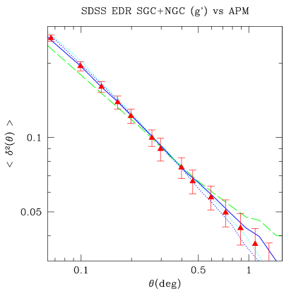
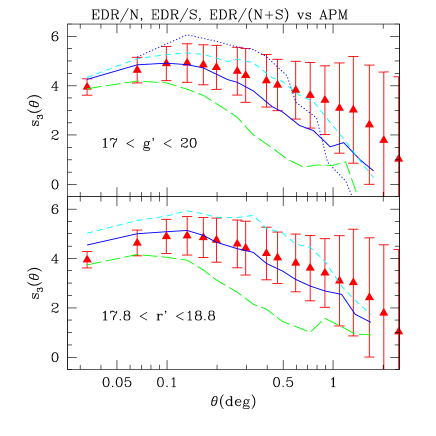
Figure 9.— Left panel: The variance $\bar{w_{2}}$ as a function of angular smoothing $\theta$. Short and long dashed lines correspond to the SDSS EDR/N and EDR/S. The dotted and continuous lines show EDR/(N+S) with and without the seeing mask. The points with errorbars show the mean and 1-sigma confidence level in the values of 10 APM sub-samples with same size and shape as the EDR/(N+S).
Right panel: Same results for the reduced skewness $s_{3}$. The top and bottom panel show the results in $g^{\prime}$ and $r^{\prime}$.

We next compare the lower order moments of counts in cells of variable size $\theta$ (larger than the pixel map resolution). We follow closely the analysis of Ga01. Fig. 9 shows the variance of fluctuations in density counts $\delta\equiv\rho/{\bar{\rho}}-1$ smoothed over a scale $\theta$: $\bar{w_{2}}\equiv<\delta^{2}(\theta)>$, which is plotted as a function of the smoothing radius $\theta$. The errors show 1-sigma confidence interval for APM subsamples with EDR/(N+S) size. The individual results in each subsample are strongly correlated so that the whole curve for each subsample scales up and down within the errors, ie there is a strong covariance at all separations due to large scale density fluctuations (eg see Hui & Gaztañaga 1999 or Eq.2 above). The EDR/(N+S) results (continuous and dotted lines) match perfectly well the APM results, in agreement to what we found for the 2-point function above. The size of the errorbars for EDR/N and EDR/S (not shown) are almost a factor of two larger than for EDR/(N+S), so that they are also in agreement with the APM within their respective sampling errors.

Right panel of Fig. 9 shows the corresponding comparison for the normalized angular skewness:

$$s_{3}(\theta)\equiv{<\delta^{3}(\theta)>\over{<\delta^{2}(\theta)>^{2}}}\equiv{\bar{w_{2}}(\theta)\over{\bar{w_{3}}(\theta)}}$$ (6)

All SDSS $g^{\prime}$ sub-samples (top panel) for $s_{3}$ show an excellent agreement with the APM at the smaller scales (in contrast with the EDSGC results, see Szapudi & Gaztañaga 1998). On larger scales the SDSS values are smaller, but the discrepancy is not significant given the strong covariance of individual APM subsamples. Note how the effect of the seeing mask (dotted line) is to increase the the amplitude of $S_{3}$, this could be partially due to systematic errors, but it could also result from the smaller, $1/3$, sampling resulting from removing the pixels with bad seeing.

Bottom panel of the left of Fig. 9 shows the corresponding results in $r^{\prime}$. At the smallest scale (of about 2’ or 240 Kpc/h) we find some slight discrepancies (at only the 1-sigma level for a single point) with the APM. The $r^{\prime}$ results seem a scaled up version of the $g^{\prime}$ results, which indicates that the apparent differences could be explained in terms of sampling effects (with strong covariance). Note also that the value of $s_{3}$ seems to peak at slightly larger scale. This could indicate another explanation for this discrepancy. Szapudi & Gaztañaga 1998 argued that such peak could be related to some systematic (or physical) effect related to the de-blending of large galaxies. It is reasonable to expect that such effect could be strong function of color, as $g^{\prime}$ and $r^{\prime}$ trace different aspects of the galaxy morphology. We have also checked that results of individual scans 756 and 94 (and also 756+94) give slightly higher results, closer to the $r^{\prime}$ results than to the mean $g^{\prime}$. Higher results are also found for the results with the seeing mask (eg dotted line in top right panel of Fig. 9). This goes in the right direction if we think that de-blending gets worse with bad seeing, but it could also be affected by sampling fluctuations (because of the smaller area in the scans or masked data).

Similar results are found for higher order moments. As we approach the scale of $2$ degrees, the width of our strip, it becomes impossible to do counts for larger cells and it is better to study the 3-point function.

3.7. 3-point Correlation function

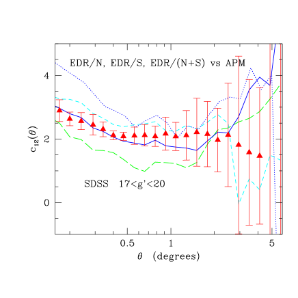
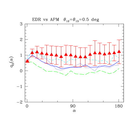
Figure 10.— Left panel: The collapsed 3-point function $c12$ as a function of galaxy separation $\theta$ for SDSS $17<g^{\prime}<20$. The short and long dashed lines correspond to the SDSS EDR/N (North) and EDR/S (South) strips. The dotted and continuous lines correspond to EDR/(N+S) with and without the seeing mask shown in Fig.7. The triangles with errorbars show the mean and 1-sigma confidence level in the values of 10 APM sub-samples ($17<B_{J}<20$) with same size as the joint EDR/(N+S) with masked seeing.
Right panel: Similar results for the 3-point function $q_{3}(\alpha)$ in isosceles triangles of side $\theta_{12}=\theta_{13}=0.5$ deg.

Following Ga01 we next explore the 3-point function, normalized as:

$$q_{3}\equiv{w_{3}(\theta_{12},\theta_{13},\theta_{23})\over w_{2}(\theta_{12})w_{2}(\theta_{13})+w_{2}(\theta_{12})w_{2}(\theta_{23})+w_{2}(\theta_{13})w_{2}(\theta_{23})}$$ (7)

where $\theta_{12}$, $\theta_{13}$ and $\theta_{23}$ correspond to the sides of the triangle form by the 3 angular positions of $\delta_{1}\delta_{2}\delta_{3}$. Here we will consider isosceles triangles, ie $\theta_{12}=\theta_{13}$, so that $q_{3}=q_{3}(\alpha)$ is given as a function of the interior angle $\alpha$ which determines the other side of the triangle $\theta_{23}$ (Frieman & Gaztañaga 1999).

We also consider the particular case of the collapsed configuration $\theta_{23}=0$, which corresponds to $<\delta_{1}\delta_{2}^{2}>$ and is normalized in slightly different way (see also Szapudi & Szalay 1999):

$$c_{12}\equiv{<\delta_{1}\delta_{2}^{2}>\over{<\delta_{1}\delta_{2}><\delta_{1}^{2}>}}\simeq 2q_{3}(\alpha=0)~{}.$$ (8)

Figure 10 shows $c_{12}$ from the collapsed 3-point function.

Note the strong covariance in comparing the EDR/N to EDR/S. The unmasked EDR/(N+S) results agree well with the APM within errors, but the results with the seeing mask (shown as the dotted line) show significant departures at small scales.

Right panel in Fig. 10 shows the reduced 3-point function $q_{3}$ for isosceles triangles of side $\theta_{12}=\theta_{13}=0.5$ degrees. Here there seems to be differences between APM and SDSS, but its significance is low because the errors at a single point is only 1-sigma and that there is a strong covariance between points, eg note how the EDR/S and EDR/N curves are shifted around the EDR(N+S) one. The APM seems closer to the EDR/N. This is a tendency that is apparent in previous figures, but it is only on $q_{3}$ where the discrepancies starts to look significant. When estimation biases are present in the subsample mean, errors tend to be unrealisticly small, that is errors are also biased down (see Hui & Gaztañaga 1999).

4. Discussion and conclusions

We have first explored the different uncertainties involved in the comparison of the SDSS with the APM, such as the band or magnitude range to use. After several test, we conclude that clustering in both the North and South EDR strips (EDR/N and EDR/S) agree well in amplitude and shape with the APM on scales $\theta<2$ degrees. But we find inconsistencies with the APM $w_{2}(\theta)$ at the level of $90\%$ significance on any individual scale at $\theta>2$ degrees. This inconsistencies are larger than $90\%$ when we compare EDR/S to EDR/N at any given point at $\theta>2$ degrees (compare the short and long dashed lines in left panel of Fig.6). We have shown that this is mostly due to systematic photometric errors due to seeing variations across the SDSS EDR (see right panel of Fig.6).

We have pushed the comparison further by combining the North and South strips, which we call EDR/(N+S) and analyze the EDR clustering as a whole. Combining samples in such a way is very risky because small systematic differences in the photometry tend to introduce large uncertainties in the overall mean surface density. This was overcome in the APM by a simultaneous match of many overlapping plates. For non-contiguous surveys the task is almost impossible, unless one has very well calibrated photometric observations, as is the case for the SDSS, to a level of 0.03 magnitudes (see Lupton etal 2001). The combined EDR/(N+S) sample shows very good agreement for the number counts (see Figure 1) and also with the APM $w_{2}(\theta)$, even at $\theta>2$ degrees. In this case the agreement is in fact within the corresponding sampling errors in the APM.

Higher order correlations show similar results. The mean SDSS skewness is in good agreement with the APM at all scales. The current SDSS sampling (1-sigma) errors range from $10\%$ at scales of arc-minutes (less than 1 Mpc/h) to about $50\%$ on degree scales ($\sim 10$ Mpc/h). At this level both surveys are in perfect agreement. The collapsed 3-point function, $c_{12}$ shows even smaller errors (this is because multi-point statistics are better sampled over narrow strips than counts in large smoothed cells). At degree scales (which correspond to the weakly non-linear regime $r\sim 8$ Mpc/h) we find $c_{12}\simeq 2.4\pm 0.6$. This amplitude and also the shape is remarkably similar to that found in simulations and what is theoretically expected from gravitational instability $c_{12}\simeq 68/21+2/3\gamma$ (see Bernardeau 1996, Gaztañaga, Fosalba & Croft 2001). The 3-point function for isosceles triangles of side $\theta_{12}=\theta_{13}=0.5$ deg. (left panel in Fig.10) seems lower than the APM values, but within the 2-sigma confidence level at any single point. Again here we would need of the covariance matrix to say more. In general, the North SDSS strip has higher amplitudes for the reduced skewness or 3-point function than the Southern strip.

We conclude that the SDSS is in good agreement with the previous galaxy surveys, and thus with the idea that gravitational growth from Gaussian initial conditions is most probably responsible for the hierarchical structures we see in the sky (Bernardeau etal 2002, and references therein).

The above agreement has encourage us to look into the detailed shape of $w_{2}(\theta)$ on intermediate scales, where the uncertainties are smaller and errors from the APM are more reliable. On scales of 0.1 to 1 degree, we find indications of slight ($\simeq 20\%$) deviations from a simple power law (this is on larger scales than the power law deviations found in Connolly etal 2001). Right panel of Fig.8 shows that the different SDSS samples have very similar slopes to the APM survey, showing a characteristic inflection with a maximum slope. In hierarchical clustering models, the initial slope of $\,d\ln\xi/d\ln r$ is a smoothed decreasing function of the separation $r$. Projection effects can partially wash out this curve, but can not produce any inflection to the shape (at least if the selection function is also regular). In Gaztañaga & Juszkiewicz (2001 and references therein) it was argued and shown that weakly non-linear evolution produces a characteristic shape in $\,d\ln\xi/d\ln r$. This shape, smoothed by projections, is evident in the APM data for $\,d\ln w(\theta)/d\ln\theta$. Here we also find evidence for such a shape in the combined EDR/(N+S) SDSS data. The maximum in the slope occurs around $\theta\simeq 0.6$ deg, which corresponds to $r\sim 5$Mpc/h, as expected if biasing is small on those scales.

In summary, both the shape of the 2-point function and the shape and amplitude of the 3-point function and skewness in the SDSS EDR data, confirms the idea that galaxies are tracing the large scale matter distribution that started from Gaussian initial conditions (Bernardeau etal 2002, and references therein).

References

- (1)
- (2) Bernardeau, F., 1994, A&A 291, 697
- Bernardeau (1996) Bernardeau, F., 1996, A&A, 312, 11 (B96)
- Bernardeau et al (2001) Bernardeau, F., Colombi., S, Gaztañaga, E., Scoccimarro, R., 2001, Physics Reports in press, astro-ph/0112551
- (5) Bernstein, G.M., 1994, ApJ, 424, 569
- (6) Connolly etal 2001, astro-ph/0107417
- (7) Dodelson, S., Narayanan, V.K., Tegmark, M, Scranton, R., etal astro-ph/0107421, submitted to ApJ.
- Frieman & Gaztañaga (1999) Frieman, J.A., Gaztañaga, E., 1999, ApJ, 521, L83 (FG99)
- Gaztañaga (1994) Gaztañaga, E., 2001, MNRASin press, astro-ph/0106379 (Ga01)
- Gaztañaga (1994) Gaztañaga, E., 1994, ApJ, 454, 561
- Gaztañaga (2000) Gaztañaga, E. & R. Juszkiewicz, 2001, R. ApJ, 558, L1
- Gaztañaga (2000) Gaztañaga, E., Fosalba, P. & Croft, R., 2001, MNRASin press astro-ph/0107523
- Gaztañaga (2000) Hui, L.& Gaztañaga, E., 1999, ApJ, 519, 622
- (14) Lupton, R., Gunn, J.E., Ivezić, Z Knapp, G.R., Kent, S., Yasuda, N, 2001, in ASP Conf. Ser. 238, Astronomical Data Analysis Software and Systems X, ed. F.R. Harnden, F.A. Primini and H.E.Payne, in press astro-ph/0101420
- Maddox (2000) Maddox, S.J., Efstathiou, G., Sutherland, W.J. & Loveday, J., 1990, MNRAS, 242, 43P
- (16) Scoccimarro, R., Feldman, H., Fry, J. N. & Frieman, J.A., 2001 ApJ, 546, 652
- (17) Scranton, R., Johnston, D., Dodelson, S., Frieman, J. etal astro-ph/0107416, submitted to ApJ.
- (18) Szapudi, I. & Gaztañaga, E., 1998, MNRAS300, 493
- (19) Szapudi, I., & Szalay, A.S., 1999, ApJ, 515 L43
- (20) Tegmark, M., Hamilton, A.J.S., Strauss, M.A., Vogeley, M.S. & Szalay, A.S. 1998, ApJ, 499, 555
- (21) Tegmark, M., etal 2001, astro-ph/0107418, submitted to ApJ.
- (22) Yasuda, N., Fukugita, M., Narayaran, V.K. etal 2001 astro-ph/0105545, submitted to ApJ.
- (23) York, D.G. etal, 2000, A.J., 120, 1579 astro-ph/0006396
- (24) Zehavi, I., Blanton, M.R., Frieman, J.A., Weinberg, D.H., Mo, H.J., Strauss, M.A., et al, astro-ph/0106476