High Resolution Simulations of the Plunging Region in a Pseudo-Newtonian Potential: Dependence on Numerical Resolution and Field Topology

Abstract

New three dimensional magnetohydrodynamic simulations of accretion disk dynamics in a pseudo-Newtonian Paczyński-Wiita potential are presented. These have finer resolution in the inner disk than any previously reported. Finer resolution leads to increased magnetic field strength, greater accretion rate, and greater fluctuations in the accretion rate. One simulation begins with a purely poloidal magnetic field, the other with a purely toroidal field. Compared to the poloidal initial field simulation, a purely toroidal initial field takes longer to reach saturation of the magnetorotational instability and produces less turbulence and weaker magnetic field energies. For both initial field configurations, magnetic stresses continue across the marginally stable orbit; measured in units corresponding to the Shakura-Sunyaev $\alpha$ parameter, the stress grows from $\sim 0.1$ in the disk body to as much as $\sim 10$ deep in the plunging region. Matter passing the inner boundary of the simulation has $\sim 10\%$ greater binding energy and $\sim 10\%$ smaller angular momentum than it did at the marginally stable orbit. Both the mass accretion rate and the integrated stress fluctuate widely on a broad range of timescales.

1 Introduction

MHD turbulence driven by magneto-rotational instability (MRI; Balbus & Hawley 1991) now appears to be the fundamental physical mechanism of angular momentum transport in accretion disks (see the review by Balbus & Hawley 1998). On the basis of this idea, it is now possible to begin to answer many questions about accretion dynamics. In a series of papers, we are investigating the global radial structure of accretion disks near the marginally stable orbit of a black hole by means of large-scale three dimensional MHD numerical simulations. In particular, we focus on the inner regions of accretion disks, and examine the time-dependence of accretion, the radial dependence of stress and dissipation, and the net energy and angular momentum per unit mass carried into the black hole. In so doing we will also need to examine more closely the conceptual basis for disk dynamics.

For understandable reasons, simple analytic models (e.g., Novikov & Thorne 1973, Shakura & Sunyaev 1973) have in general been built on the assumption of time-steadiness. However, this assumption is by no means a given in real disks. Even if there is a long-term mean accretion rate, it is entirely possible for there to be short-term fluctuations. In fact, sizable fluctuations seen in the light-curves of every accreting black hole indicate that accretion variability is the norm, not the exception (e.g., Sunyaev & Revnivtsev 2000).

The difficulty with addressing issues of time-dependent dynamics within the context of traditional analytic models is that the dynamics of accretion depend fundamentally on the nature of the stress that transports angular momentum. While many steady-state or time-averaged properties of disks may be adequately described by a simple stress parameterization (e.g., the Shakura-Sunyaev $\alpha$ prescription in which the stress is supposed proportional to pressure), the actual dynamics cannot be so treated. $\alpha$ is only a measure of the stress; it is not the physics behind the stress. Within the $\alpha$ parameterization, stress results from turbulent fluctuations (not viscosity). These fluctuations have amplitudes less than or of order the sound speed $c_{s}$ on scales less than or of order the disk scale-height $H$. Again, while there may be regions of the disk where it is sufficient to time-average over these fluctuations, this cannot be the case near the black hole where accretion time- and length-scales become comparable to those that characterize the turbulence. Direct dynamical simulations are required to understand time-dependent quantities.

Although it has long been clear that ordinary viscosity cannot account for angular momentum transport in accretion disks, modeling the stress “as if” it were viscous has been a popular way of thinking about disks for an equally long time. Again, for dynamical issues this is clearly incorrect: a low-viscosity plasma that is turbulent does not behave like high-viscosity laminar flow. A separate question is whether the turbulent stress would behave sufficiently similarly to viscosity that there would be an associated dissipation rate proportional to the local stress (Novikov & Thorne 1973; Shakura & Sunyaev 1973). Not all stresses have this property, although if the MRI-driven MHD turbulence dissipates locally in a turbulent cascade it is amenable to an $\alpha$-type description (Balbus & Papaloizou 1999). Because we now know that the dominant stress is electromagnetic, local dissipation is not certain; Poynting flux can easily carry energy from one place to another, and highly-magnetized coronae and winds may account for much of the liberated energy. Numerical simulations offer the possibility of measuring to what degree this happens.

Both the radial dependence of stress and dissipation and the net energy and angular momentum delivered to the black hole depend on yet another plausible, but not demonstrated, assumption: that the inter-ring stress disappears in the vicinity of the marginally stable orbit. Two heuristic arguments were raised in behalf of this assumption: that the small amount of mass in the plunging region could hardly be expected to exert a force on the far heavier disk proper (Novikov & Thorne 1973, Page & Thorne 1974); and if the stress scales as a constant fraction $\alpha$ of the local pressure, then the low pressure in the plunging region would lead to a very small stress (Abramowicz & Kato 1989). However, as recognized by Page & Thorne (1974), neither of these arguments applies to magnetic stresses. Krolik (1999) and Gammie (1999) argued that the dominant role of magnetic stresses in angular momentum transport in the disk body should actually lead to stresses near the marginally stable orbit large enough to substantially alter the amount of energy and angular momentum removed from matter before it passes through the black hole’s event horizon. If so, the radial distribution of stress in the disk would also be significantly altered, with wide-ranging observational consequences (Agol & Krolik 2000). Simulations can quantitatively evaluate the importance of this mechanism.

Global three-dimensional disk simulations have only recently become possible, and the number of such models is still sufficiently small that it remains possible to give a nearly comprehensive list of references: Armitage (1998); Matsumoto (1999); Hawley (2000, hereafter H00); Machida et al. (2000); Hawley & Krolik (2001, hereafter HK01); Hawley (2001); Armitage et al.  (2001). All of this work has shared two key assumptions: Newtonian dynamics in a Newtonian or pseudo-Newtonian (Paczyński-Wiita) potential, and a fixed (adiabatic or isothermal) equation of state. All of this work has also struggled with the same central problem: obtaining resolution adequate to describing the physics.

In this paper, we report simulations with the best resolution in the inner accretion flow yet achieved. We also use these simulations to explore whether the topology of the initial seed magnetic field has any lasting effects on the structure of the accretion flow. In later efforts we will improve the level of realism in these simulations by solving the energy equation and employing genuine relativistic dynamics.

2 Numerical Method

As in past work (H00; HK01) we evolve the equations of Newtonian MHD in cylindrical coordinates $(R,\phi,z)$, namely

$${\partial\rho\over\partial t}+\nabla\cdot(\rho{\bf v})=0$$ (1)

$$\rho{\partial{\bf v}\over\partial t}+(\rho{\bf v}\cdot\nabla){\bf v}=-\nabla\left(P+{\mathcal{Q}}+{B^{2}\over 8\pi}\right)-\rho\nabla\Phi+\left({{\bf B}\over 4\pi}\cdot\nabla\right){\bf B}$$ (2)

$${\partial\rho\epsilon\over\partial t}+\nabla\cdot(\rho\epsilon{\bf v})=-(P+{\mathcal{Q}})\nabla\cdot{\bf v}$$ (3)

$${\partial{\bf B}\over\partial t}=\nabla\times\left({\bf v}\times{\bf B}\right)$$ (4)

where $\rho$ is the mass density, $\epsilon$ is the specific internal energy, ${\bf v}$ is the fluid velocity, $P$ is the pressure, $\Phi$ is the gravitational potential, ${\bf B}$ is the magnetic field vector, and ${\mathcal{Q}}$ is an explicit artificial viscosity of the form described by Stone & Norman (1992a). To model a black hole gravitational field we use the pseudo-Newtonian potential of Paczyński & Wiita (1980) which is

$$\Phi=-{GM\over r-r_{g}},$$ (5)

where $r$ is spherical radius, and $r_{g}\equiv 2GM/c^{2}$ is the “gravitational radius,” akin to the black hole horizon. For this potential, the Keplerian specific angular momentum (i.e., that corresponding to a circular orbit) is

$$l_{kep}=(GMr)^{1/2}{r\over r-r_{g}},$$ (6)

and the angular frequency $\Omega=l/R^{2}$. The innermost marginally stable circular orbit is located at $r_{ms}=3r_{g}$. We use an adiabatic equation of state, $P=\rho\epsilon(\Gamma-1)=K\rho^{\Gamma}$, where $P$ is the pressure, $\rho$ is the mass density, $\epsilon$ is the specific internal energy, $K$ is a constant, and $\Gamma=5/3$. Radiation transport and losses are omitted. Since there is no explicit resistivity or physical viscosity, the gas can heat only through adiabatic compression or by artificial viscosity which acts in shocks.

The code employs time-explicit Eulerian finite differencing. The numerical algorithm is that of the ZEUS code for hydrodynamics (Stone & Norman 1992a) and MHD (Stone & Norman 1992b; Hawley & Stone 1995). We set $GM=1$ and $r_{g}=1$ (so that $c=\sqrt{2}$), thus establishing the units of time and velocity. The circular orbital period at a radius $r$ is $P_{orb}=2\pi\Omega^{-1}=2\pi r^{3/2}(r-r_{g})/r$.

In this paper we increase the overall resolution within the disk itself and in the inflow region above what was used in H00 and HK01. The computational grid is laid out in cylindrical coordinates, with $256\times 64\times 192$ zones in $R\times\phi\times z$. This represents only a 50% increase in the total number of zones used compared to HK01. In the present simulations, however, the zones are concentrated to increase the effective resolution in the most important regions of the flow. We locate more of the zones near the marginally stable orbit and around the equator, and double the angular resolution while decreasing the angular extent. The radial inner boundary is moved in to $R_{\rm min}=1.25$ and there are 110 equally spaced zones out to $R=4$. Compared to our earlier simulation, this scheme decreases the zone size $\Delta R$ in the inner region by a factor of 3.3. Beyond $R=4$, $\Delta R$ gradually increases; the remaining 146 zones extend out to $R=36$. The $z$ coordinate is centered on the equatorial plane, and runs from -11 to $+11$. From $z=-1$ to $1$ there are 76 equally spaced zones; again comparing to the earlier simulation, the $\Delta z$ around the equator is smaller by a factor of 2.4. Beyond $z=\pm 1$, $\Delta z$ gradually increases out to the top and bottom boundaries.

The angle $\phi$ spans the range from 0 to $\pi/2$ in 64 equally spaced zones; $\Delta\phi$ is half the size used in H00 and HK01. Although the resolution is improved over H00 and HK01, the domain is only one quarter as large. However, experiments (Hawley 2001) with “cylindrical” disks (no vertical gravity) found that reducing the angular domain from $2\pi$ to $\pi/2$ does not alter the qualitative features of the evolution, although it lowered the energy and stress levels by about 10%. Since the practical advantage of limiting the angular domain is great, we use it here and assume that the quantitative effects will be small.

The boundary conditions on the grid are simple zero-gradient outflow conditions; no flow into the computational domain is permitted. The magnetic field boundary condition is set by requiring the transverse components of the field to be zero outside the computational domain, while the perpendicular component satisfies the divergence-free constraint. The $\phi$ direction is, of course, periodic.

The initial condition for the simulations is the same torus used in HK01 and for model GT4 of H00. This is a moderately thick torus ($H/R\simeq 0.12$ at the pressure maximum) with an angular velocity distribution $\Omega\propto R^{-1.68}$, slightly steeper than Keplerian. The angular momentum within the torus is equal to the Keplerian value at the torus pressure maximum at $R=10$. As before, the pressure and density at $R=10$ are $P_{max}=0.036$ and $\rho_{max}=34$, while $P_{orb}(R=10)=179$. For reference, the orbital period at the marginally stable orbit is $P_{orb}=21.8$.

We consider two different initial field configurations: poloidal loops, as in HK01 and H00, and a purely toroidal field. These models are discussed in turn in §3 and §4.

3 Initially Poloidal Magnetic Field

The initial magnetic field topology for the the first of the two simulations reported here is identical to that of the GT4 simulation in H00 and the simulation presented in HK01: poloidal field loops lying along equal density surfaces in the torus. The initial condition for the magnetic field is set by the toroidal component of the vector potential $A_{\phi}(R,z)=\rho(R,z)-\rho_{min}$, for all $\rho$ greater than a minimum value, $\rho_{min}=0.1$. The poloidal field is then obtained from ${\bf B}=\nabla\times{\bf A}$. The resulting field is fully contained within the torus. The strength of the magnetic field is set so that the ratio of the total integrated gas pressure to magnetic pressure is 100, i.e., $\beta=P_{\rm gas}/P_{\rm mag}=100$.

Only three differences distinguish this simulation from the previous ones: the earlier simulations treated a full $2\pi$ in azimuth, whereas this one considers only a single quadrant; the gridding scheme used in the new one offers an improvement of roughly a factor of 3 in $R$ and $z$ resolution, and a factor of 2 in $\phi$ resolution; and the new simulation was run somewhat longer, to $t=1838$ rather than $t=1500$. This longer time corresponds to 84 orbits at $r_{ms}$, and is reached in 560,000 timesteps. Two purposes are served by studying this new simulation: we examine the degree to which the higher resolution of the new simulation allows us to approach numerical convergence, and it provides a standard of comparison for the simulation reported in the next section whose initial magnetic field was purely toroidal.

Just as in earlier simulations, the poloidal field loops of the initial state have unstable MRI wavelengths that are well-resolved on the grid. As a result, the MRI grows rapidly and turbulence develops within the disk. The disk expands as the MHD turbulence redistributes angular momentum. When the inner edge reaches the marginally stable orbit, matter begins to accrete through the inner boundary of the simulation, into the “black hole”. The initial growth phase of total field energy ends at $t\simeq 600$. For the remainder of the simulation, conditions in the disk exhibit a rough stationarity, but with very large fluctuations in almost every quantity. The disk is modestly thick with $H/R\simeq 0.21$ at $R=10$ and $H/R\simeq 0.15$ at $R=3$.

We begin quantitative consideration of this simulation with its mass accretion history. In the GT4 simulation the mean time-averaged accretion rate was 4 in code units. In the HK01 simulation, the mean accretion rate was very nearly 5; in the new simulation, the mean accretion rate rises to $\simeq 6.4$ (fig. 1a). In all cases the accretion rate is characterized by large fluctuations with time. However, the amplitude of the fluctuations is larger in the new simulation. In the previous, lower-resolution work, the typical peak/trough ratio was $\simeq 1.1$–1.2; in the new one this ratio approaches 2.

As before, we also examine the Fourier power spectrum of the time-varying accretion rate. We previously found that the power spectrum was a smooth function of frequency that gradually steepened towards higher frequencies; its mean logarithmic slope over two decades in frequency was $\simeq-1.7$. In this new simulation, the power spectrum is quite similar, but exhibits slightly less curvature. From the lowest frequency ($f\simeq 10^{-3}$ inverse time units) up to roughly the orbital frequency at $r_{ms}$ (0.046 inverse time units) $|\hat{\dot{M}}|^{2}\propto f^{-1}$; from that frequency up to $f\simeq 1$, the logarithmic slope is $\simeq-2$ (fig. 1b). A small local peak appears at around a period of 41, which corresponds to the circular orbit frequency at $R=4.2$. The significance of this peak is unclear; if it is a real feature, it might be interpreted as suggesting that the final “plunge” into the black hole is controlled by events a short way outside the marginally stable orbit. This would not be surprising as the size of the fluctuations in the MHD turbulence in this region is of the same order as the local scale height and the turbulence timescale is comparable to the infall time. However, it is also possible that the peak is a statistical fluctuation.

Figure 1: Upper panel: Mass accretion rate at the inner edge as a function of time in the initially poloidal simulation. Lower panel: Solid line is Fourier power density per logarithmic frequency interval of the accretion rate into the black hole (i.e. $\log(f|\widehat{\dot{M}}|^{2}$). Dashed line is Fourier power in the same units for the volume-integrated Maxwell stress. To avoid transients associated with the initial start up and linear growth phase, the spectrum is computed for $t\geq 600$ time units.

The shape of the Maxwell stress power spectrum is different. It, too, may be described as a broken power-law, but in this case $|\widehat{M_{r\phi}}|^{2}\propto f^{-2}$ at high frequencies, while bending to a steeper slope at low frequencies. In shearing-box simulations, the power spectrum of the fluctuating Maxwell stress is also a power-law of index -2 over several decades in frequency around the local orbital frequency; it therefore appears that the dominant stress fluctuations in these global simulations are controlled primarily by local effects. Note that the observable fluctuating quantity, the luminosity, may be more closely related to the stress than to the accretion rate because it is tied to the dissipation rate. However, it is further modified by the distribution of photon escape times.

The origin of the larger accretion rate seen in this simulation is a stronger magnetic field (fig. 2) which produces a greater $R$-$\phi$ stress. As we also found in HK01, the field strength is typically somewhat greater near the disk surface than in the equatorial plane. Compared to the HK01 simulation, the azimuthally-averaged energy density in magnetic field increased by 50% in the accreting portion of the disk ($R\leq 10$, $|z|\leq 4$); at larger radius the net flow is outward, and there is little mass or field at higher altitude. The stress is also larger than in HK01, both in absolute terms and as a fraction of the disk pressure. Figure 3 compares the azimuthally-averaged, vertically-integrated magnetic stress and gas pressure at the endtime of the HK01 simulation to the same quantities in this new simulation. In both cases, although the pressure has a clear maximum as a function of radius (as happens in almost every disk model due to the sharp inward drop in density as the radial velocity grows near $r_{ms}$), the magnetic stress increases monotonically inward. However, the magnitude of the stress is everywhere greater in the higher resolution simulation; it is 2.8 times larger at $r_{ms}$. In addition, the pressure gradient is slightly shallower when better resolution is employed.

Figure 2: The azimuthally-averaged magnetic pressure, $\langle B^{2}/8\pi\rangle_{\phi}$, measured at the end-time in the initially poloidal simulation, plotted on a logarithmic scale from $10^{-3.5}$ to $10^{-1.5}$. Fig. 11 shows the same quantity in the initially-toroidal simulation.

Figure 3: Vertically-integrated and azimuthally-averaged pressure and magnetic stress at time $t=1490$ in two initially-poloidal simulations. The solid curve shows the $R$-$\phi$ magnetic stress in the simulation of HK01; the dotted curve shows the pressure in the same simulation. The dashed and dot-dashed curves show the magnetic stress and pressure, respectively, in the new higher-resolution simulation. Analogous data for the initially-toroidal simulation are shown in fig. 12.

A popular way of parameterizing the importance of the magnetic stress is through the Shakura-Sunyaev “$\alpha$” parameter. In its original definition (Shakura & Sunyaev 1973), the disk is supposed to be azimuthally symmetric and time-steady, and $\alpha$ is given by the ratio of the vertically-integrated $R$-$\phi$ component of the stress tensor to the vertically-integrated disk pressure. Although it remains useful to compare observed stress levels to the pressure, there is no unique way (or most physically significant way) to define $\alpha$ in non-symmetric MHD turbulence. One may compute it as a local quantity at each point in $R$, $\phi$, and $z$ or one may average it in any of a variety of ways. Different definitions and averaging procedures yield quantitatively distinct results. However, certain trends do show consistent behavior.

For example, as already suggested in Figure 3, there is a general rise toward smaller radii in the importance of magnetic stresses relative to pressure stresses. Defining $\alpha_{SS}$ as the azimuthal average of the ratio between the vertically-integrated magnetic stress $-B_{R}B_{\phi}/4\pi$ and the vertically-integrated pressure, we find (see fig. 4) that $\alpha_{SS}$ is typically $\simeq 0.1$ – 0.2 in the accretion portion of the disk that is well outside $r_{ms}$ (i.e., $5\leq R\leq 10$). Inside $R=5$, it rises sharply, reaching $\simeq 0.5$ near $R=3$, and approaching $\sim 10$ at the innermost edge of the simulation. In the earlier simulation, $\alpha_{SS}\simeq 0.06$–0.08 between $R=5$ and $R=10$, rising inside $R=3$, but always at a lower level than the new simulation.

The “hump” in $\alpha_{SS}$ around $R=20$ is also seen in the HK01 simulation, but with smaller amplitude. The hump arises because the magnetic pressure generally has a larger scale height than does the gas pressure. As a result, in the outer portion of the disk the stress also falls less rapidly with $R$ than the gas pressure, creating a peak in $\alpha$ outside the gas pressure maximum.

If one chooses to parameterize the stress by the total pressure, gas plus magnetic, the rise is less dramatic. The definition of $\alpha$ that yields the most constant value is stress divided by magnetic pressure, $\alpha_{mag}\equiv-2B_{R}B_{\phi}/B^{2}$. This has a value between 0.2 and 0.3 throughout the main part of the disk, and rises slowly toward 1 inside $R=6$. This definition of $\alpha$ measures the degree of correlation between the toroidal and radial components of the field. Because the shear has a consistent sense, the turbulence is anisotropic and $\langle B_{R}B_{\phi}\rangle\neq 0$. The value within the disk is typical for stress arising from MHD turbulence. However, $\alpha_{mag}$ increases through the plunging region as turbulence gives way to more coherent fluid flow. Here the field evolves primarily through flux-freezing and the strong correlation created by shear is only weakly diminished by turbulence.

Figure 4: Azimuthally- and time-averaged ratio of the vertically-integrated stress to: the vertically-integrated gas pressure, i.e., $\alpha_{SS}$ (top solid curve); the gas plus magnetic pressure (bottom solid curve); and the magnetic pressure, i.e., $\alpha_{mag}$ (dashed line) in the initially poloidal simulation. The time-average runs from $t=1500$ to the end of the simulation.

These results highlight the limitations of the $\alpha$ picture: the stress doesn’t actually correlate particularly well with the pressure. Another drawback to parametrizing the stress as an averaged $\alpha$ is that doing so obscures its highly variable nature. There is tremendous irregularity in the distribution of stress with altitude and azimuth (fig. 5). At a fixed radius within the accreting portion of the disk, the azimuthally-averaged stress can vary by more than an order of magnitude within plus or minus two gas scale-heights from the midplane; similarly, the vertically-integrated stress may vary by comparable amounts as a function of azimuth. Often, but not always, the stress is greater near the disk surface than in its midplane.

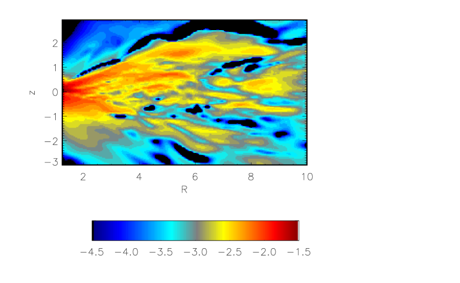
Figure 5: Logarithm (base 10) of the azimuthally-averaged magnetic stress at a late-time in the initially poloidal simulation. The largest, most consistent stresses are associated with the plunging region near and within the marginally stable orbit. In the black regions of the plot, the azimuthally-averaged stress is negative, i.e., it is attempting to transport angular momentum inward. However, the magnitude of the largest azimuthally-averaged negative stress is at most only $\sim 10^{-3}$ in these units.

Another way to look at the radial stress distribution is with the “scaled stress.” In a steady-state disk, the local vertically-integrated $R$-$\phi$ stress must be equal to the mass accretion rate times the difference between the local specific angular momentum $l(R)$ and the specific angular momentum carried into the black hole $l(r_{g})$, i.e.,

$$\bar{S}={\dot{M}\Omega(R)\over 2\pi}\left[1-{l(r_{g})\over l(R)}\right],$$ (7)

where $\dot{M}$ is the total mass accretion rate, $\Omega(R)$ the rotational frequency, and $l$ is the specific angular momentum. the quantity in square brackets is sometimes called the “reduction factor”.

In HK01, we found that the time- and azimuthally-averaged magnetic stress very nearly matched the stress predicted by (7) for the time-averaged mass accretion rate in the body of the disk, but, in sharp contrast to the prediction of the conventional zero-stress model, maintained a high level from $R=5$ to the inner edge of the simulation at $R=1.5$.

In the higher-resolution simulation the stress behaves in a similar, but not quite identical, fashion. In particular, the finer resolution leads to increased stress near the marginally stable orbit. In figure 6, the time-averaged, azimuthally-averaged, and vertically-integrated stress is scaled by $\langle\dot{M}\rangle\Omega/2\pi$ in order to highlight its effective “reduction factor”, i.e. the amount by which the stress is diminished due to the outward angular momentum flux. Note that for this purpose, $\Omega$ is the usual orbital frequency for a circular orbit outside $r_{ms}$, but inside $r_{ms}$ it is the actual orbital frequency as determined by the angular momentum and radial position of the material. In the figure, $\Omega$ inside $r_{ms}$ is approximated by assuming that the angular momentum is constant in the plunging region; this approximation (as shown in the following paragraphs) depresses the result by about 5% in the mean.

The scaled stress represents the contrast between the local specific angular momentum and the accreted angular momentum per accreted mass. In a time-steady disk this quantity would approach unity at large radius, but in the simulation it is considerably smaller than 1 there because the finite outer edge in our mass distribution leads to a strong inconsistency there with the time-steady approximation. Angular momentum is being transferred into the outer disk, which is moving outward in response. By definition, in a time-steady disk the scaled stress must be zero at the innermost boundary; the conventional model predicts that it goes to zero at $R=3$ and stays zero at all smaller radii. In the simulation, the scaled stress tracks the conventional model fairly well between $R=12$ and $R=5$, but at smaller radii, instead of going sharply to zero at $R=3$, it falls more gradually: between $R=1.25$ and $R=5$ it is $\propto R^{1.3}$. This continuing importance of magnetic stress in the inner portions of the disk is a counterpart to the increase in $\alpha_{SS}$ that occurs at the same place.

Figure 6: Azimuthal- and time-averaged scaled magnetic stress as a function of radius (solid curve) contrasted with the prediction of the zero-stress boundary condition model (dashed curve). As in Figure 4, the time average starts at $t=1500$.

The result of this continuing stress is a transfer of both angular momentum and energy from the plunging region inside $R=3$ to the disk proper at greater radius. As shown in Figure 7, the mean specific angular momentum falls by about 5% inside the marginally stable orbit, while the mean binding energy per unit mass rises by about 10–20%. These significant, but modest, changes in the mean hide the much larger amounts of angular momentum and energy transfer that can occur in individual fluid elements. Some individual fluid elements arrive at $R=1.3$ with binding energy almost twice the mean binding energy at $R=3$, while others pass the “event horizon” with slightly positive net energy (fig. 8). Because the magnetic stress has a vertical scale-height roughly twice the gas density scale-height, the torque per unit mass felt by matter near the disk surface is greater than that expressed in the midplane; in consequence, the specific angular momentum is systematically smaller off the equatorial plane, often by 10–20%. In nonstratified cylindrical disk simulations (Armitage et al. 2001; Hawley 2001) the decline of $l$ inside of $r_{ms}$ can be significantly reduced. A systematic study of the influences of gas pressure (i.e., $H/R$) and computational domain size carried out by Hawley (2001) suggests that stratification plays a dominant role in determining $dl/dR$ inside of $r_{ms}$ and the present simulation supports that conclusion. Even with nonstratified disks, however, strong fields near $r_{ms}$ can produce substantial torques and reductions in $l$ (Reynolds, Armitage & Chiang 2001).

Figure 7: Mass flux weighted azimuthally- and vertically-averaged specific binding energy (solid curve) and angular momentum (dashed curve) at the end of the initially poloidal simulation. Both curves are normalized to their values at $R=3$ to emphasize the continuing change at smaller radii. The spikes in the binding energy just outside the inner radius of the simulation are artifacts.

Figure 8: Net energy in rest-mass units in a slice through the equatorial plane in the plunging region at late time in the initial poloidal field simulation. Note that in these units the binding energy of a circular orbit at $r_{ms}$ is 0.0625.

Figure 8 illustrates another aspect of the character of the flow inside $r_{ms}$: as gas plunges toward the “event horizon”, transfers of energy and angular momentum between adjacent fluid elements become stronger and stronger. Orbital shear stretches initially coherent regions into spirals stretching roughly a radian in azimuth. Local contrasts become especially strong deep in the plunging region because gas there can no longer exert forces and torques on gas farther out.

Viewed in a poloidal slice (fig. 9), the simulation reveals a different effect: in the plunging region, gas is concentrated where the magnetic shear or current density is particularly great. Interestingly, this concentration is much less noticeable considered as a function of azimuth. Generally speaking the gas and magnetic pressures are anticorrelated in the disk (although within the disk the gas pressure is generally larger). The total pressure is much smoother than either the gas or magnetic pressure separately.

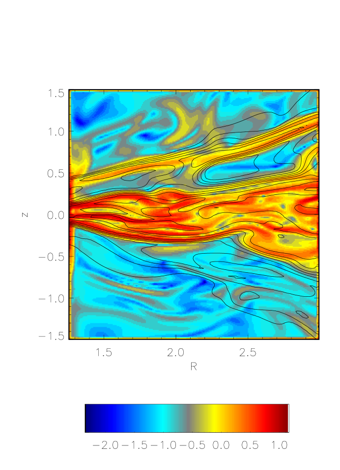
Figure 9: Magnitude of the electric current (color contours) compared with gas density (line contours) in a poloidal slice at $\phi=\pi/4$, both in a logarithmic scale. The two quantities are very well correlated.

4 Initially Toroidal Field

The second simulation begins with the same initial torus as before, but with a purely toroidal magnetic field. The most appropriate field topology in accretion disks is not known a priori and this simulation investigates how much the results depend on the initial field structure. We believe (as we discuss at greater length below) initially toroidal and initially poloidal fields bracket the range of possibilities.

The initial field configuration has toroidal field with a plasma $\beta=10$ wherever $\rho\geq 0.1$. The model was run at two resolutions. One was the same as described above with $256\times 64\times 192$ zones. This disk was evolved for 800,000 timesteps to time $t=2704$ (124 orbits at $r_{ms}$). The other, a lower resolution comparison simulation, is discussed below in §5.1.

The toroidal field simulation evolves in significantly different ways from the initially poloidal field case. First, with no initial radial field there is no shear amplification of the toroidal component during the early stages of the evolution. Second, the most unstable wavenumbers of the linear toroidal field MRI are different from those of the vertical field. For a pure toroidal field the fastest growth rates correspond to azimuthal wavenumber $m\sim v_{\phi}/v_{A}$ (i.e., $m$ is large for typical subthermal field strengths) and large poloidal wavenumbers (Balbus & Hawley 1992; Terquem & Papaloizou 1996; Kim & Ostriker 2000). In previous local and global simulations done with a toroidal field (Hawley, Gammie, & Balbus 1995; H00), small scale fluctuations appear first, followed gradually by larger scale turbulence. As a result of these effects, the torus evolves more slowly than with a poloidal field, and the field energy and stress levels at saturation are smaller. In the present simulation the period of linear growth and evolution occupies the first $\sim 1000$ time units.

Nonetheless, the evolution of the disk after $\sim 1000$ units is in many ways qualitatively similar to the initially-poloidal simulation. Angular momentum is transported outward and its distribution evolves toward Keplerian. Smaller field energies and stresses cause the toroidal disk to be thinner than the poloidal field disk, with $H/R$ remaining comparable to the initial value 0.12 at $R=10$ and $H/R\simeq 0.1$ inside $R=5$. Just as for the initially-poloidal simulation, there is substantial accretion through the inner cylindrical boundary and hardly any mass loss through the outer boundaries.

From $\sim 1000$ time units to the end, the accretion rate ranges between $\simeq 0.5$ and 2.5, i.e., between 8% and 40% of the accretion rate in the initially poloidal simulation (fig. 10). In contrast to the accretion rate history of the poloidal simulation, $\dot{M}$ builds slowly and features relatively smooth swings from a “low state” to a “high state” and back again. The ratio between the high and low accretion rates can be as large as $\sim 3$; there is no time at which $\dot{M}$ could fairly be said to be approximately stationary. In the poloidal case there are also large fluctuations between high and low rates, but these occurred on shorter timescales. Here there seems also to be a secular increase in $\dot{M}$ after $t=1000$, but its significance is hard to gauge as any long-term trend is masked by the very large fluctuations that occur. Figure 10b is the Fourier power spectrum of the initially-toroidal accretion rate. It strongly resembles the power spectrum of the initially poloidal simulation, both with regard to its broken power-law character and the existence of a small peak (which in this simulation is at the slightly greater period of 47, corresponding to the circular orbit frequency at $R=4.5$). A second peak can be seen at a period of 142, which is the circular orbital frequency associated with $R=8.7$. The significance of these peaks is as uncertain as that of the similar peak found in the Fourier power spectrum of the initially-poloidal accretion rate.

Figure 10: Upper panel: Mass accretion rate at the inner edge as a function of time in the initially toroidal simulation. Lower panel: Fourier power density per logarithmic frequency interval of the accretion rate into the black hole (solid curve), and Fourier power density per logarithmic frequency interval of the volume-integrated Maxwell stress (dashed curve). To avoid transients associated with the initial start up and linear growth phase, the spectrum is computed for $t\geq 1000$ time units.

Because the accretion rate varies so much during this simulation, no single time can fairly represent its behavior. We will discuss two “snapshots”, one from a low accretion rate stage (at 2704 time units, when the accretion rate through the inner edge was $\simeq 1$), the other from a time of high accretion rate (2537 time units, when the accretion rate was 2.4).

In previous initial toroidal field simulations, both global and local, saturation occurs at lower turbulent field energies than models beginning with poloidal components. This is true in the present simulation as well. The azimuthally-averaged field strength (fig. 11) is about 10% stronger in the “high rate” case compared to the low. Both, however, are about six times smaller than in the poloidal simulation when averaged over the accreting portion of the disk ($R\leq 10$, $|z|\leq 4$). In addition, the vertical scale height of the magnetic field is roughly half what it was in the initially poloidal case.

Figure 11: Azimuthally-averaged magnetic energy density in the “high accretion rate” snapshot (upper panel) and the “low rate” snapshot (lower panel). The scales in these two figures are identical to the scale used in fig. 2 to ease comparison.

Not surprisingly, given the generally weaker magnetic field, the effective $\alpha_{SS}$ is significantly smaller in the toroidal case than in the poloidal. In the poloidal simulation (fig. 4), $\alpha_{SS}\simeq 0.1$ at $R=10$ and rises sharply inward to a peak of almost 10 at the inner boundary. In the two toroidal snapshots, $\alpha_{SS}\simeq 0.01$ – 0.03 near $R=10$, and, although rising inward, it reaches a maximum of only $\simeq 0.2$–0.3 just inside the marginally stable orbit. This contrast, of course, accounts for the lower accretion rate in the toroidal case, despite having initially an identical mass surface density. The value of $\alpha_{mag}$, the ratio of the magnetic stress to the magnetic pressure, is 0.2–0.3 in the disk, rising from that value to $\sim 1$ from $R=4$ to the event horizon. This is similar to the poloidal field case, except that the systematic increase begins at a slightly smaller radius.

Comparatively weaker magnetic field also leads to a different shape to the stress distributions (fig. 12). The radial pressure gradient is much larger in the toroidal field case than in the poloidal field simulation: the vertically-integrated pressure falls by roughly a factor of 30 from $R=10$ to $R=3$, whereas the decline was only about a factor of 3 in the initially poloidal run. The magnetic stress, which rose steadily inward in the poloidal case, is approximately flat here between $R=15$ and $R=5$ and falls by about a factor of two from $R=5$ to $R\simeq 2$–3, inside of which it is again constant.

Figure 12: Vertically-integrated and azimuthally-averaged pressure and magnetic stress at late times in the high and low accretion rate snapshots from the initially toroidal simulation. The solid curve shows the $R$-$\phi$ magnetic stress in the high accretion rate case; the dotted curve shows the pressure at the same time. The dashed and dot-dashed curves show the magnetic stress and pressure, respectively, in the low accretion rate snapshot.

Although the magnetic stress is generally weaker in the toroidal simulation than in the poloidal one, the mean change in specific angular momentum inside the marginally stable orbit is similar to that found in the poloidal simulation: a drop of 5 – 10% (fig. 13). On the other hand, the detailed character of the angular momentum distribution in the plunging region is quite different in the initially toroidal simulation. As we have already remarked, the change in energy and angular momentum of individual fluid elements is much greater than the mean change. When the accretion rate is especially high in the toroidal simulation, the contrast in specific angular momentum between adjacent fluid elements is much greater than when the accretion rate is low (fig. 14). Instead of passing through the inner boundary with specific angular momentum 2.6 (the angular momentum of the marginally stable orbit), in the high accretion rate case there are streams arriving with as little as $\simeq 1.8$ and some that arrive with as much as $\simeq 3$. By contrast, during the time of low accretion rate, the range is only from $\simeq 2.2$ – 2.6.

The energy of accreting matter behaves in similar fashion, but with some notable contrasts. At the time of high accretion rate, the mean binding energy increases gradually from $R=3$ to $R=2$ to a maximum that is about 10% greater than at the marginally stable orbit, while at the time of low accretion rate there is little change in mean binding energy in the plunging region. However, just as in the poloidal simulation, the slow change in mean energy masks very large changes in the energy of individual fluid elements (fig. 15). As with the angular momentum, the energy exchange inside $R=2$ is much stronger in the case of initially toroidal field: whereas the maximum increase in binding energy in the poloidal case was about a factor of two, in the toroidal case it is a factor of 10 – 20! Finally, in all cases, there is a spike in the mean binding energy just outside $R_{min}$ that is an artifact of the boundary condition.

Figure 13: Mass flux weighted azimuthally- and vertically-averaged specific binding energy and angular momentum as functions of radius in the initially toroidal simulation. The solid curve shows binding energy in the high accretion rate state, the dotted curve angular momentum; the dashed and dash-dotted curves are energy and angular momentum, respectively, in the low accretion rate state. All four curves are normalized to their values at $R=3$ to emphasize the continuing change at smaller radii. The spikes in the binding energy just outside the inner radius of the simulation are artifacts.

Figure 14: Mass-weighted vertically-averaged specific angular momentum in the inner part of the accretion flow for the initially toroidal case: upper panel, at high accretion rate; lower panel, at low accretion rate.

Figure 15: Net energy in rest-mass units in a slice through the equatorial plane in the plunging region during the time of high accretion rate in the initially toroidal simulation.

5 Discussion

5.1 Field topology

5.1.1 Stress distribution

We suggest that the contrasting behavior seen in the toroidal and poloidal field simulations illustrates the effects of different inflow and magnetic dissipation times. The ratio between these two quantities distinguishes the disk proper from the plunging region. In the disk proper, the inflow time is long compared to the dissipation time so that turbulent dissipation controls the magnetic stress; on the other hand, in the plunging region the inflow time is short compared to the dissipation time so that the field and stress evolve primarily through flux-freezing.

The shearing-box approximation corresponds to the disk proper because the inflow time is effectively infinite. In those simulations (Hawley, Gammie & Balbus 1995, 1996), the magnetic field tends to saturate at a roughly constant $\beta$ value with respect to the local pressure. The stress is then a fixed fraction $\alpha_{mag}$ of the field energy density. We find just this sort of behavior in the portion of our simulations well outside $r_{ms}$, with $\alpha_{mag}\simeq 0.2$–0.3 in the initially-poloidal simulation and somewhat smaller in the initially-toroidal case.

However, in our simulations $\alpha_{mag}$ increases steadily toward unity from $R\simeq 5$ to the inner boundary, indicating a qualitative change in the nature of the accretion flow at this radius. At small radii, the inflow time diminishes while the dissipation time (we expect) does not change greatly. Where the inflow time is shorter than the dissipation time, the field evolves via shear amplification and flux-freezing and is decoupled from the local pressure. The dominance of coherent shear over turbulence accounts for the increase in $\alpha_{mag}$.

The contrast between the initially-poloidal and initially-toroidal cases arises from the fact that the inflow time at any given radius of the disk proper is longer in the toroidal simulation than in the poloidal due to the weaker magnetic stress. As a result, the zone in which the field energy density roughly tracks the pressure extends further inward when the initial field is purely toroidal. The magnetic stress in the toroidal run begins to evolve via flux-freezing at a smaller radius than in the poloidal run and (crudely) follows the diminishing pressure between $R=6$ and $R=3$, whereas in the poloidal run the magnetic stress continues increasing inward even when the pressure is decreasing.

In evaluating these contrasts, however, it is essential to remember that the dissipation rate in these simulations is controlled by numerical, not physical effects (see further discussion in §5.2); consequently, our results may not be quantitatively reliable guides to the behavior of real disks.

5.1.2 Which field topology is “natural”

From these simulations it appears that the level of stress at and inside the marginally stable orbit depends significantly upon whether the initial field topology is toroidal or poloidal. Dependence of the level of MHD turbulence on initial field topology has been observed in previous simulations, both global and local. The linear analysis of the MRI shows that the fastest growing wavelengths of vertical fields are axisymmetric and have larger vertical wavelengths, while the toroidal field instability is nonaxisymmetric, favors small wavelengths, and grows transiently as time-dependent radial wavenumbers swing from leading to trailing. Given these differences it is important to ask which field topology better represents the state of an actual accretion flow.

A result that is common to all of the simulations done to date, both global and local, is that the toroidal field energy dominates the final turbulent state, whatever the initial field configuration. This does not mean, however, that the initial purely toroidal field evolution is the best model; it is in many ways a singular state, and there are sharp differences between it and models that have even a small amount of local net poloidal field. For example, Hawley et al. (1995) carried out several local shearing box runs in which a very much weaker vertical field was added to boxes with strong toroidal fields. The result was greatly enhanced turbulence. As noted by Hawley (2000) even if global simulations begin with no overall net poloidal field, but include some poloidal field in the form of field loops, local regions of the disk still behave like local simulations with poloidal fields, that is they generate strong turbulence and $\alpha\sim 0.1$.

Hence, if an accretion flow begins from a source with even a small amount of poloidal field, and that field remains in or is amplified by the resulting inflow, one would expect local regions of the disk to behave more like the poloidal field simulation than like the pure toroidal field case. Given the strong influence of even a weak poloidal field, the inner disk dynamics could well be variable over long timescales due to variations in the net poloidal field carried in by accretion from the outer disk. Nonetheless, in a time-average sense we expect real disks to resemble the initially-poloidal simulation more than the initially-toroidal simulation.

5.2 Influence of resolution

The contrast between our new results and those obtained from the previous simulations of HK01 and H00 provides a measure of the effects of numerical resolution (Table 1). The grid used in HK01 is, in its inner parts, finer by a factor 1.9 in $\Delta R$ and 2.5 in $\Delta z$ relative to the grid of simulation GT4 in H00; our new grid is finer by a factor 3.3 in $\Delta R$, a factor 2.4 in $\Delta z$ and 2.0 in $\Delta\phi$ relative to the simulation of HK01. We have also done a second initially-toroidal simulation with lower resolution than the one described in §4. It used $128\times 32\times 128$ grid zones. The radial grid concentrated 55 zones linearly spaced inside $R=4$; outside this point $\Delta R$ gradually increased to the outer boundary at $R=32$. The vertical grid put 40% of the zones within $\pm 2$ of the equator, with a graded mesh beyond that point out to $z=\pm 8.8$. Thus in the lower resolution toroidal simulation $\Delta R$ is twice as large, and $\Delta z$ three times as large in the inner disk region. This model was run for 400,000 timesteps to time $t=3873$.

Table 1: Inner Disk Region Resolutions

Simulation	$\Delta R$	$\Delta z$	$\Delta\phi$
GT4 (H00)	0.16	0.16	0.05
HK01	0.083	0.0625	0.05
new poloidal	0.025	0.026	0.025
new toroidal	0.025	0.026	0.025
low-res. toroidal	0.05	0.077	0.05

It should be noted that, since this is a study of the disk structure near $r_{ms}$, we have focused the resolution improvements within the inner regions of the flow and around the equator. To the extent that the overall evolution depends on the outer parts of the disk, the effective resolution difference between simulations is far less than that of the inner region. The resolution in the outer disk of HK01 is actually poorer than that in the same portion of GT4.

5.2.1 Accretion rate

With two successive improvements in resolution by roughly factors of 3, the mean accretion rate in the initially-poloidal case increased 60% from GT4 to HK01 and a further 30% in the new simulation. The increase in accretion rate between HK01 and the new simulation might have been slightly greater if the new simulation had spanned a full $2\pi$ in azimuthal angle, rather than being restricted to only a single quadrant. Moreover, the fluctuations about the mean also increased substantially with improving resolution, with the peak to trough ratio increasing from $\simeq 1.1$ to $\simeq 2$.

A similar rise in accretion rate with increasing resolution was seen in the pair of initially-toroidal simulations. At the lower resolution, the time-averaged accretion rate was $\simeq 0.7$, fluctuating between a high of 1.7 and a low of 0.3. By contrast, with better resolution the accretion rate (after the end of transient effects) had a mean of 1.7 and fluctuated between 0.5 and 2.6.

These numerical experiments show that increasing resolution produces increased stress and accretion rates. For the poloidal field simulation the observed time-steady mean accretion rate is probably within tens of percent of the “converged” value, although almost certainly still on the low side. However, we have not yet achieved sufficient resolution to gauge the convergence of the magnitude of the fluctuations around the mean. For the simulation with the initial toroidal field, the increase in $\dot{M}$ with resolution was sufficiently great that it is not yet possible to estimate what the converged value might be.

5.2.2 Magnetic field

Between GT4 and HK01 there was a dramatic increase in magnetic field energy density in the inner disk: roughly a factor of 10. However, the improvement in resolution between HK01 and the new simulation, although comparable in magnitude to that between GT4 and HK01, changed the magnetic field much less: an increase of about 50% in mean energy density.

Analogous effects can be seen in the toroidal case. Growth to turbulent saturation takes almost twice as long, and the averaged poloidal field energies (a measure of the strength of the turbulence) in the saturated state are reduced by about a factor of 2 in the poorer resolution simulation.

Stronger magnetic field is mirrored in a rising ratio between magnetic stress and gas pressure. In the stable part of the accretion region (i.e., $5\leq R\leq 10$), $\alpha_{SS}\simeq 0.05$–0.1 in HK01 and 0.1–0.2 in the new poloidal simulation. The initially-toroidal simulations show an increase from $\simeq 0.01$–0.028 in the lower-resolution simulation to $\simeq 0.02$–0.03 in the higher-resolution run.

It appears very likely that improvements in resolution reduce numerical dissipation of magnetic field. Because of the central role of magnetic torques in driving accretion, the stronger magnetic field then increases the accretion rate. On the basis of the decline in the rate of increase of the magnetic field energy density with resolution in going from HK01 to our new poloidal simulation, it appears that, with regard to the mean field intensity, we are approaching convergence for the poloidal case, but it is likely that further refinement would yield at least modest quantitative changes.

We have less confidence that the initially-toroidal case is sufficiently well-resolved. As noted above, the toroidal field MRI favors high wavenumbers, precisely those that are the most challenging to resolve. The resolution comparison carried out here suggests that even with the higher resolution grid the simulation is not yet converged, and the values reported here must be regarded as lower bounds.

5.2.3 Stress distribution

As we discussed at length in §5.1, the ratio between effective magnetic dissipation time and inflow time plays a critical role in governing the magnitude of stresses in the inner disk. Where the dissipation time is short compared to the inflow time, the magnetic field strength is coupled to the local pressure; where the comparison is reversed, the field evolves by flux-freezing. At even our finest resolution, the dissipation rate is exaggerated by numerical effects. Consequently, in these simulations the magnetic field intensity is tied to the pressure further in than would be expected in a real disk where flux-freezing would set in at a larger radius. Thus, the stress observed in these simulations at small radii is most likely still undervalued.

5.2.4 Energy conservation

Energy conservation and energy flow can be difficult for a finite difference simulation to compute accurately when there are significant departures from equipartition in energy components. Here the bulk of the energy is gravitational and orbital; thermal energy is only 2% of the total at the beginning of the simulation, and 4% at the end. Thermal, magnetic, and poloidal kinetic energy combined are only 14% of the circular orbit binding energy at $r_{ms}$ at the end of the simulation. Small errors in the gravitational and orbital energy can, in principle, then lead to large errors in the other elements of the energy budget. However, to answer the questions of interest, an accurate accounting of magnetic, thermal, and random kinetic energies is important.

In real disks, the energy of matter reaching the event horizon is determined by a competition between several rates: of energy transfer via work done on other matter and magnetic fields; of turbulent dissipation; of magnetic reconnection; of photon creation; and of photon diffusion. The rate of energy transfer via work is determined by the structure of the large-scale magnetic field and fluid motions. Turbulent dissipation is due to a two-part process: nonlinear wave interactions transfer energy from long wavelengths to short, where they can in turn be dissipated into heat by resistivity and viscosity. Magnetic reconnection is controlled by the rate at which fluid motions force together fluid elements with oppositely directed magnetic field. When the gas is heated, a variety of processes (bremsstrahlung, Compton scattering, etc.) transfer its heat into photon energy. Finally, energy leaves the disk as photons diffuse away.

Generally speaking, in these simulations we account reasonably accurately for large-scale energy transfer, overall disk evolution, and the long-wavelength portion of the turbulent cascade. However, numerical effects substitute for small-scale dissipation and enhance reconnection. Because the nonlinear wave interaction rate on long lengthscales is very rapid compared to the numerical dissipation rate, the effective turbulent dissipation rate in the simulation is controlled by numerical effects. Radiation we ignore entirely, with regard to both photon creation and photon diffusion. The absence of a real treatment of dissipation and photon losses hinders our ability to estimate the energy released by accretion. For example, in HK01 we argued that the observed change in energy between $R=3$ and $R_{min}$ was likely to be an underestimate because, in the absence of radiative losses, some of the work done by plunging matter on gas farther out would eventually be brought back in.

However, at some level numerical effects mimic radiation by causing energy to be lost when converging fluid elements carry with them oppositely directed velocity or magnetic field. We can estimate the relative importance of numerical energy losses by a simple argument. If energy were exactly conserved locally, the only change in the integrated energy over the problem area would be due to material that flows off the grid. Here that effectively means material accreted because, for example, over the course of the poloidal simulation 19% of the initial mass passes through the inner boundary while only 1.5% leaves through the outer boundary. The binding energy of the accreted matter is, on average, about 0.118 in our units, so that mass-loss alone should increase the energy by 0.0224 if the initial mass is defined as unity. Starting from a total energy of -0.042, that means the final energy should be -0.0196. However, we actually find a final energy of -0.0272. The difference (a loss of 0.0076) can be attributed to numerical losses. Because the numerical dissipation time is shorter than the inflow time over much of the disk, this total energy loss is very close to the total radiation loss predicted by the conventional model, but there is no reason to believe that the specific location and rate of numerical losses in the simulation accurately predict what would happen in a real disk.

5.3 Stress at the marginally stable orbit

In these simulations we observe stress at the marginally stable orbit, yet it has been a long-standing belief that the stress must be close to zero at that point. As discussed in §1, at least two such arguments have been put forward in support of this notion. One is that the flow in the plunging region would necessarily be low density and would lack the inertia necessary to exert a torque on the disk (Novikov & Thorne 1973; Page & Thorne 1974). However, Page & Thorne point out that this argument doesn’t apply if the torques are carried by magnetic fields.

The second argument relies upon the $\alpha$ stress model, i.e., that the stress is $\alpha\rho c_{s}^{2}$. This point is worth revisiting in slightly more detail. Equation (7) relates the mass accretion rate to the stress in a steady state accretion flow. Using the $\alpha$ model for the stress, this equation can be rewritten

$$\alpha_{SS}(c_{s}/v_{R})(c_{s}/R\Omega)=\Delta l/l(R)$$ (8)

where $\Delta l$ is the difference between the local angular momentum $l(R)$ and the angular momentum carried into the hole, $l(r_{g})$. Once the inflow passes $r_{ms}$, the inflow speed increases and the pressure drops precipitously, and with it the stress according to the $\alpha$ prescription. The $\alpha$ model is implicitly hydrodynamic, so the point at which plunging matter loses contact with the disk is the sonic point. There, by definition, $v_{R}\sim c_{s}$, and $c_{s}/R\Omega=H/R<1$. Since $\alpha_{SS}$ is generally thought to be considerably less than unity, it would seem to follow that $l$ changes very little in the plunging region. This is the basis for the “proof” that the stress goes to zero at $r_{ms}$.

In the simulations, however, we find a scaled stress, i.e. $\Delta l/l$, at $r_{ms}$ that is $\approx 0.05$ – 0.1. Why does the proof fail? Because the reasoning used relies on a strict application of the $\alpha$ relation, that is, that the pressure determines the stress. But the magnetic stress in the plunging region doesn’t depend upon the gas pressure; $\alpha$ climbs rapidly inside $r_{ms}$ as the gas pressure drops and the field evolves mainly by flux freezing. In fact, we find in the initially poloidal simulation that $\alpha_{SS}$ increases by a factor of 100 as matter falls through this zone.

Since the torque is magnetic, can we save relation (8) by replacing gas pressure with magnetic pressure, and setting the torque equal to $\alpha_{mag}\rho v_{A}^{2}$? Even with this readjustment, $\alpha$ still doesn’t determine the stress in a manner that can be used in a proof; $\alpha_{mag}$ is also not a constant in the plunging region. It is roughly constant with value 0.2–0.3 in the disk proper where magnetic turbulence is active, but rises toward 1 in the plunging region. The stress in the plunging region becomes more efficient relative to the magnetic pressure as the radial field is stretched out in the inflow, and its strength relative to the toroidal field grows. Moreover, $v_{A}/(R\Omega)$ increases slowly inward in the flux-freezing regime, whereas in the conventional $\alpha$ model $c_{s}/(R\Omega)$ falls rapidly inward.

These problems illustrate the difficulties that can arise when the $\alpha$ formalism is taken too literally. The $\alpha$ parametrization cannot be used as the basis of a proof. At best, it might be possible to use the reformulated version of this argument using $\alpha_{mag}$ to estimate a time-averaged $\Delta l/l$. In that case, the observed change in $l$ of 5–10% inside the plunging region is consistent with the value of $v_{A}/(R\Omega)$ that we find ($\simeq 0.15$ for the poloidal field case, $\simeq 0.05$ for the toroidal field case).

6 Conclusion

In this paper we report on two new three-dimensional MHD global accretion disk simulations, one beginning with a poloidal field and the other with a purely toroidal field. Since the topology of the magnetic field in a real disk is largely unknown (except for the observation that it is almost certainly dominated by the toroidal component) these two initial configurations are intended to bracket the possible range. We find that initial field topology makes a significant quantitative difference in the resulting evolution. With a purely toroidal field, initial field amplification is slower, and the saturation energies, magnetic stresses, and accretion rate are smaller, The magnetic stress begins to evolve by flux freezing at a smaller radius in the toroidal field run. However, the qualitative features of angular momentum transport and stress at the marginally stable orbit are unchanged. In any event, we expect that because the MRI is so effective at amplifying poloidal field, real disks are likely to resemble the initially-poloidal simulation more than the purely toroidal one.

We reexamined the issue of stress at the marginally stable orbit, and confirmed our previous finding (HK01) that the stress remains significant there. The character of the stress changes as the flow moves from turbulence to inflow. Within the body of the disk, where the dissipation time is short compared to the inflow time, the field evolves by MRI-driven MHD turbulence limited by dissipation (numerical in the simulation, resistive and viscous in real disks). The relative correlation of $B_{R}$ and $B_{\phi}$ ($\alpha_{mag}$) in that regime is $\simeq 0.2$–0.3. As the flow approaches $r_{ms}$ from the outside, the inflow time falls until it is shorter than the dissipation time. Inside that radius, the field evolves mainly via flux freezing and $\alpha_{mag}$ increases toward unity. The location of this transition is one of the most important parameters governing the character of the inner accretion flow. As a result of the continuing stress in the plunging region, inside $r_{ms}$ accreting matter suffers a modest ($\sim$10%) decline in its average specific angular momentum and a comparable increase in its binding energy. Rapid variability in accretion rate remains the rule with the most power at frequencies lower than the orbital frequency at $r_{ms}$.

These simulations used the largest number of grid zones and arranged them so as to achieve the finest resolution in the inner accretion flow of any simulation to date. We find that the increased resolution used in these simulations produced increased field energy and stress, and also lead to larger amplitude variations in the accretion rate. We believe that at this level of resolution we are approaching numerical convergence with respect to the magnetic field intensity and the accretion rate for the initially-poloidal case, but finer resolution may be necessary to demonstrate convergence for these quantities when the initial field topology is toroidal, and for other quantities for both topologies. Unfortunately, it is difficult to obtain significantly greater resolution or to use this high resolution over a wider range of radius. Certain questions will therefore remain difficult to answer for some period of time (most importantly, the location of the dissipation/flux-freezing transition radius). Perhaps this is not surprising, considering that we are attempting to resolve a turbulent cascade within a global disk. On the other hand, the overall evolution and qualitative features have remained consistent from the lowest to highest resolutions. This is fortunate since the dynamics of self-consistent MHD accretion flows remain largely unexamined, and further exploration with even the modest resolution permitted by current practical considerations is likely to be fruitful.

- (1) Abramowicz, M.A., & Kato, S. 1989, ApJ, 336, 304
- Agol & Krolik (2000) Agol, E., & Krolik, J.H. 2000, ApJ, 528, 161
- Armitage (1998) Armitage, P.J. 1998, ApJ, 501, L189
- Armitage (2001) Armitage, P.J., Reynolds, C.S., & Chiang, J. 2001, ApJ, 548, 868
- Balbus & Hawley (1991) Balbus, S.A., & Hawley, J.F. 1991, ApJ, 376, 214
- Balbus & Hawley (1992) Balbus, S.A., & Hawley, J.F. 1992, ApJ 400, 610
- Balbus & Hawley (1998) Balbus, S.A., & Hawley, J.F. 1998, Rev Mod Phys, 70, 1
- Balbus & Papaloizou (1999) Balbus, S.A., & Papaloizou, J. C. B. 1999, ApJ, 521, 650
- Gammie (1999) Gammie, C.F. 1999, ApJ, 522, L57
- Hawley (2000) Hawley, J.F. 2000, ApJ, 528, 462 (H00)
- Hawley (2001) Hawley, J.F. 2001, ApJ, 554, 534
- Hawley, Gammie & Balbus (1995) Hawley, J.F., Gammie, C. F., & Balbus, S.A. 1995, ApJ, 440, 742
- Hawley, Gammie & Balbus (1996) Hawley, J.F., Gammie, C. F., & Balbus, S.A. 1996, ApJ, 464, 690
- Hawley & Krolik (2001) Hawley, J.F., & Krolik, J.H. 2001, ApJ, 548, 348 (HK01)
- Hawley & Stone (1995) Hawley, J. F., & Stone, J. M. 1995, Comp Phys Comm, 89, 127
- Kim & Ostriker (2000) Kim, W.-T., & Ostriker, E.C. 2000, ApJ, 540, 372
- Krolik (1999) Krolik, J.H. 1999, ApJ, 515, L73
- Machida et al. (2000) Machida, M., Hayashi, M. R., & Matsumoto, R. 2000, ApJ, 532, L67
- Matsumoto (1999) Matsumoto, R. 1999, in Numerical Astrophysics, eds. Miyama, S., Tomisaka, K. & Hanawa, T (Kluwer: Dordrecht), 195
- Novikov & Thorne (1973) Novikov, I.D., & Thorne, K.S. 1973, in Black Holes, eds. C. de Witt, & B. de Witt (New York: Gordon & Breach), 343
- Paczyński & Wiita (1980) Paczyński, B., & Wiita, P. J. 1980, A&A, 88, 23
- Page & Thorne (1974) Page, D.N., & Thorne, K.S. 1974, ApJ, 191, 499
- Reynolds, Armitage & Chiang (2001) Reynolds, C. S., Armitage, P. J., & Chiang, J. 2001, in Proceedings of the 20th Texas Symposium, eds. J. C. Wheeler & H. Martel, in press
- Shakura & Sunyaev (1973) Shakura, N. I., & Sunyaev, R. A. 1973, A&A, 24, 337
- (25) Stone, J. M., & Norman, M. L. 1992a, ApJS, 80, 753
- (26) Stone, J. M., & Norman, M. L. 1992b, ApJS, 80, 791
- Sunyaev & Revnivtsev (2000) Sunyaev, R., & Revnivtsev, M. 2000, A&A, 358, 617
- Terquem & Papaloizou (1996) Terquem, C., & Papaloizou, J. C. B. 1996, MNRAS, 279, 767