Luminosity and Variability of Collimated Gamma-ray Bursts

Abstract

Within the framework of the internal shock model, we study the luminosity and the variability in gamma-ray bursts from collimated fireballs. In particular we pay attention to the role of the photosphere due to $e^{\pm}$ pairs produced by the internal shock synchrotron photons. It is shown that the observed Cepheid-like relationship between the luminosity and the variability can be interpreted as a correlation between the opening angle of the fireball jet and the mass included at the explosion with a standard energy output. We also show that such a correlation can be a natural consequence of the collapsar model. Narrow jets, in which the typical Lorentz factors are higher than in wide jets, can produce more variable temporal profiles due to smaller angular spreading time scales at the photosphere radius. Using a multiple-shell model, we numerically calculate the temporal profiles of gamma-ray bursts and show that our simulations reproduce the observed correlation.

1 Introduction

Gamma-ray bursts (GRBs) and the afterglows are well described by the fireball model (e.g. see Piran 2000), in which an explosive flow of relativistic matter (ejecta) is released from a central engine. The collision of fast-moving ejecta with slower ejecta results in a GRB. Thereafter, the ejecta shocks and sweeps up a large amount of ambient matter. The shocked matter powers the long-lived afterglow.

The temporal profiles of GRBs are often very variable and each profile looks very different. Quantitative measures of the variability have been suggested allowing for a systematic study of their morphology. Several studies have explored the possibility that quantities directly measurable in GRB light curves could be related to the luminosities of the bursts. Stern, Poutanen & Svensson (1999) concluded that there is an intrinsic correlation between luminosity and the complexity of GRBs. Ramirez-Ruiz & Fenimore (1999; see also Fenimore & Ramirez-Ruiz 2000) found that the luminosities of seven bursts with known redshifts are correlated with the variabilities. Based on this work, Reichart et al. (2001) also reported a possible Cepheid-like luminosity estimator for long bursts. Using the GRB rate density derived from this correlation, Lloyd-Ronning, Fryer & Ramirez-Ruiz (2001) discussed the star formation rate at high redshift.

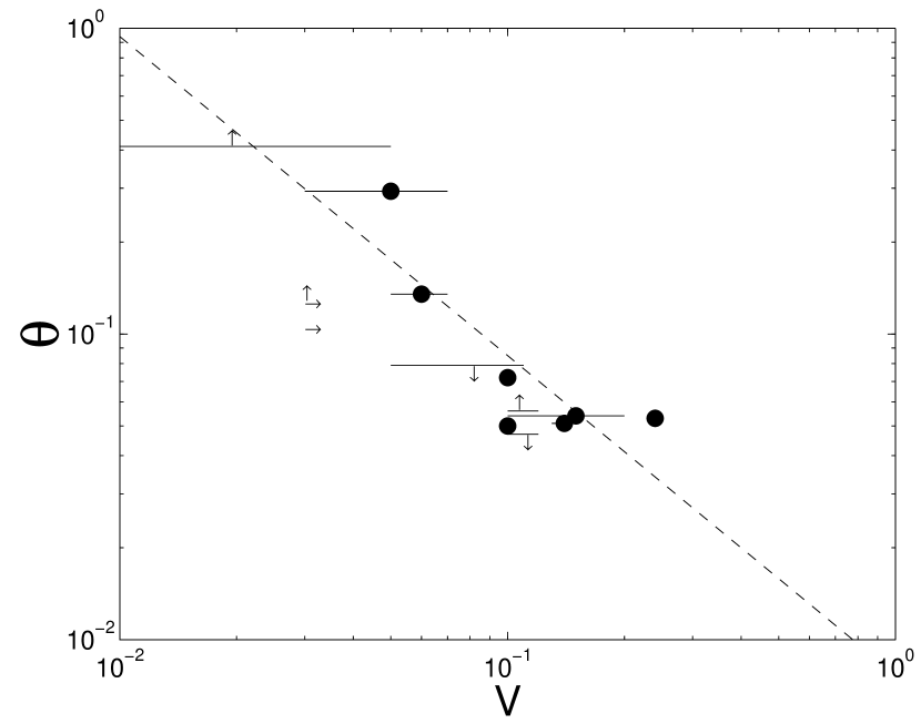
Figure 1: Opening Angle vs. Variability: Measurements (filled circles) and upper or lower limits (arrows) are shown from Reichart et al (2001) and Frail et al (2001). A linear fit to filled circles gives $\theta\propto V^{-1.0}$.

Recent afterglow observations allow us to determine the geometry of ejecta, whether it is spherical or conical. There is excellent observational evidence that the ejecta have conical geometry (jet), and there appears to be a correlation in the sense that the bursts with the largest gamma-ray fluences have the narrowest opening angles. The correlation is improved when the fluences are all scaled to the same distance by using the redshift measurements. Frail et al. (2001), Panaitescu & Kumar (2002) and Piran et al.(2001) reported that the gamma-ray energy releases, corrected for geometry, are narrowly clustered around $10^{51}$erg, and suggested that the wide variation in fluences and luminosities of GRBs is due entirely to a distribution of the opening angles. If this is the case, the Cepheid-like relation implies a correlation between the opening angle and the variability: more highly collimated GRBs are more variable. Such a correlation is actually found in the observations (see figure 1).

As a result of relativistic beaming, an observer can see only a limited portion of the ejecta. There should be no observable distinction between a spherical ejecta and a conical ejecta until the ejecta has slowed down in the afterglow phase. Therefore, the correlation between variability and opening angle should be attributed to the properties of the central engine. In this paper, we will explore the relations among variability, luminosity and jet opening angle in the framework of the internal shock model. We show that the variability-opening angle relation and the Cepheid-like relation can be interpreted as a correlation between the opening angle and the mass included at the explosion. In §2 we first discuss the collapsar model as the central engine of GRBs. In §3 we make some comments on the typical GRB energy. In §4 we discuss the internal shocks and the temporal profile. In §5 we study internal shocks by using a multiple-shell model. In §6 we consider what assumptions are actually require to fit the Cepheid-like relation. In §7 we give conclusions.

2 Central Engine: Collapsar

While the nature of the GRB progenitors is still unsettled, it now appears likely that at least some bursts originate in explosions of very massive stars (main sequence mass $M_{ms}>25~{}M_{\sun}$). The model currently favoured for long bursts is the collapsar model in which GRBs are caused by relativistic jets expelled along the rotation axes of collapsing massive stars. The jets are powered by a black hole with a surrounding accreting torus. Energy from the accretion is pumped into jets via electrodynamic processes or by neutrino annihilation. In addition spin energy of the rotating black hole may be tapped by magnetic fields anchored in the accretion disk.

According to Frail et al. (2000), Panaitescu & Kumar (2002) the wide variation in the fluences of GRBs originates from the differences in opening angles of the jets. A wide jet radiates gamma-ray photons into a large solid angle, resulting in a dim burst. Though we do not know yet what physical mechanism results in the wide variation of the opening angles, it is likely that a wider jet involves a larger mass at the explosion, and that it results in a flow with a lower Lorentz factor.

In the collapsar model, the duration of a GRB is set by the collapse time scale of a massive stellar core, typically $\sim 10$ sec for helium cores of $8<M_{\alpha}<15$. The progenitor has a mass $>25~{}M_{\sun}$ on the main sequence but loses its envelope to a binary companion and/or stellar wind before core collapse. The stellar core is assumed to collapse to a black hole, due to it’s large mass, and to be rotating sufficiently rapidly to form an accretion disk around the newly born black hole (Woosley 1993; MacFadyen & Woosley 1999).

Typical accretion disk time scales are milliseconds and gas typically resides briefly in the accretion disk. The key point is that the disk is continuously fed by the collapsing star. Short time scales are available and indeed expected due both to variability in accretion rate and the jet instabilities as the hot jet material expands along the polar axis of the star and interacts with the surrounding star.

For disks forming with radius $\sim 10^{7}$ cm, typical accretion time scales are t${}_{acc}\sim 0.01$ sec. Fluctuations in accretion rate due to instabilities were shown to exist with 50 msec time scales (MacFadyen & Woosley 1999). In models where accretion energy is tapped to power relativistic polar jets, these fluctuations in accretion may translate into variation in jet Lorentz factor perhaps leading to variation in the GRB light curves. However time scales calculated so far in numerical simulations are probably too short to produce the observed variations.

A more promising source of time structure in GRBs are instabilities arising as a relativistic jet propagates through the stellar mantle. Instabilities in the flow due to shear between the jet and the star or backflow from the jet head result in fluctuating jet speeds. Recent numerical simulations of relativistic jets propagation through collapsars demonstrate the presence of the variability some with time scales of $\sim 0.1$ sec (Zhang, Woosley & MacFadyen).

MacFadyen, Woosley & Heger, 2001 (hereafter MWH) showed that jets of equivalent energy injected into a stellar envelope can be focussed by the pressure of the star. The degree of focusing is a function of the assumed entropy of the jet which was parametrized by $E_{int}/E_{tot}$. “Colder” jets were squeezed into tightly collimated flow while “hotter” jets of the same energy expanded sideways (See MWH Fig 10). The result was that “hotter” jets are broader and sweep up a larger mass of stellar material along the rotation axis of the star. While the calculations in MWH were non-relativistic, the results should hold in special relativity since the asymptotic Lorentz factor is an inverse function of the swept up mass. Current fully relativistic numerical simulations indicate the results do hold (Zhang, Woosley & MacFadyen).

MWH also experimented with the effect of the collapsar density structure on jet collimation and found a large difference in jet opening angle for two density structures corresponding to low and high disk mass. The difference was due to the assumed viscosity parameter, but may also result from initial angular momentum and density structure of the progenitor stars. Calculations of the collapsar density structures and their effect on relativistic jet opening angle are currently underway.

3 Typical GRB energy

In the collapsar model, the energy powering the GRB originates in an accretion torus surrounding a rotating black hole of several solar masses. The stellar progenitor must lose its envelope in order to have a sufficiently small radius to allow a relativistic jet formed near the accreting black hole to pierce the star in a GRB time scale i.e. $R_{*}<10sec~{}(c/2)\sim 1.5\times 10^{11}$ cm. In addition the range of angular momentum conducive to GRB formation may be narrow. It is constrained on the low end by the angular momentum sufficient to form a disk and on the upper end, so that the disk is small enough to cool at least partially by neutrino emission (though these neutrino need not participate directly in jet formation). Disks which are inefficiently cooled are convective leading to outflows and inefficient accretion (MacFadyen & Woosley 1999; Narayan et. al). The successful GRB-producing collapsars may therefore be expected to have roughly similar energetics.

Another requirement for GRB production is that the jets have sufficient momentum flux to overcome the ram pressure of the column of gas accreting along the stellar rotation axis. Since the momentum flux decreases with a larger opening angle, there is a maximum opening angle which will not be swamped by the accretion ram. Equivalently for a given opening angle there is a minimum momentum flux capable of launching a jet. Given an observed maximum jet opening angle, this sets a lower limit for energy flux capable of producing a GRB. Given a similar typical time scale this implies a similar total energy.

4 Internal Shocks and the Temporal Structure

Internal shocks arise in a relativistic wind with a nonuniform velocity when the fast moving flow catches up the slower one. The wind can be modelled by a succession of relativistic shells (Kobayashi, Piran & Sari 1997, hereafter KPS). A collision of two shells is the elementary process, and produces a single pulse of gamma-ray. Three time scales, the cooling time, the hydrodynamic time and the angular spreading time, are relevant to the pulse width. With the relevant parameters the cooling time is negligible compared to the other two time scales (Sari, Narayan & Piran 1996). Let $d$ and $D$ be the width and separation of the shells. In other words, we assume that the central engine operates for a period $d/c$ and then is quiet for a period $D/c$. The hydrodynamic time scale $\sim d/c$ and the angular spreading time scale $\sim D/c$ determine the rise and the decay time of the pulse, respectively. Since most observed pulses rise more quickly than they decay, the pulse width is mainly determined by the angular spreading time $\sim D/c$ (Norris et al. 1996 ; Ryde & Petrosian 2001).

The whole light curve of a GRB is given by the superposition of the resulting pulses from each collision. Since all shells are moving towards us with almost speed of light, we observe pulses arising from collision between shells mostly according to their positions inside the wind, i.e., according to the time when those shells were emitted by the central engine (KPS; Nakar & Piran 2001). The relative positions of the shells inside the wind are also determined by the separations. Therefore, the variability time scales in the temporal profile reflect the shell separations at the central engine well.

The observed distribution of peak separations $\{D/c\}$ has a large dispersion (Nakar & Piran 2001). While the fastest variability time scale in GRBs is about a millisecond, the largest peak separations or the total durations are usually very much longer. Long bursts have durations from 10 to 1000sec. Clearly, whatever is the physical mechanism behind the GRB production, it acts on a much longer timescale than the fastest dynamical time. Many GRB models involve accretion onto a compact object, usually a black hole. If the accretion disk is fed by fallback of material after a supernova explosion, as in the collapsar model, then the duration and large peak separations are determined by fallback, not the dynamical accretion time. The large dispersion of peak separations could be explained in the collapsar model.

It has recently been shown that the Thomson optical depth due to $e^{\pm}$ pairs produced by synchrotron photons plays an important role in the internal shock model (Guetta, Spada & Waxman 2001; Asano & Kobayashi 2002). In order to obtain high radiative efficiency and the characteristic clustering of spectral break energies of GRBs in the range 0.1-1 MeV, the collision radii are required to be similar to the photosphere radius. Since collisions producing narrow pulses occur at small radii $\propto D$, the photosphere might obscure these, leaving only the wider pulses visible. This will make the temporal profile smooth. In a wider jet, the typical Lorentz factor $\Gamma$ is smaller, a larger fraction of the collisions occur at small radii $\propto\Gamma^{2}$ below the photosphere, therefore, the smoothing effect is expected to be stronger. This might explain the correlation between luminosity and variability in GRBs.

5 Shell Model

We discuss the smoothing effect by using a multiple-shell model. We represent the irregular wind by relativistic shells in a manner similar to that in KPS. Because of the relativistic beaming effect, we can study the emission from a jet by using spherical shells with an isotropic explosion energy $E_{iso}(\theta)=4E/\theta^{2}$ where $E$ is the geometrically corrected explosion energy and $\theta$ is the opening angle. The gamma-ray energy released from a GRB is narrowly clustered around $10^{51}$erg (Frail et al. 2001), and the conversion efficiency from the explosion energy into the gamma-rays is about $10\%$ (Guetta, Spada & Waxman 2001; Kobayashi & Sari 2001). Then, $E\sim 10^{52}$ erg.

5.1 Two-Shell Collision and Photosphere

Consider a two shell collision which is the elementary process in the multiple shell evolution. A rapid shell with Lorentz factor $\Gamma_{r}$ and mass $m_{r}$ catches up to a slower one with $\Gamma_{s}$ and $m_{s}$, and the two merge to temporarily form a single shell. Using conservation of energy and momentum we calculate the Lorentz factor of the merged shell to be

$$\Gamma_{m}\sim\sqrt{\frac{m_{r}\Gamma_{r}+m_{s}\Gamma_{s}}{m_{r}/\Gamma_{r}+m_{s}/\Gamma_{s}}}.$$ (1)

The internal energy of the merged shell is the difference of kinetic energy before and after the collision, $E_{int}=m_{r}c^{2}(\Gamma_{r}-\Gamma_{m})+m_{s}c^{2}(\Gamma_{s}-\Gamma_{m})$. We assume that electrons are accelerated to a power-law distribution of Lorentz factor $\gamma_{e}$, with a minimum Lorentz factor $\gamma_{m}$: $N(\gamma_{e})d\gamma_{e}\propto\gamma_{e}^{-p}d\gamma_{e},\gamma_{e}\geq\gamma_{m}$. Throughout this paper, we use the standard choice $p=2.2$. A constant fraction $\epsilon_{B}$ of the internal energy goes into magnetic energy. The energy distributed to the electrons is radiated via synchrotron emission.

A significant fraction of the kinetic energy could be converted to the internal energy if the relative velocity of the two shells is relativistic. However, it is not reasonable that all the internal energy is emitted, because electrons do not have most of the internal energy, and protons do not cool. Defining $\epsilon_{e}$ as the fraction of energy given to electrons, we expect $\epsilon_{e}<1$. Even at equipartition with protons $\epsilon_{e}$ is $1/2$

If $\epsilon_{e}<1$, the merger produced by a collision is expected to stay hot after the emission. As a result, the merger will spread, transforming the remaining internal energy back to kinetic energy. Kobayashi and Sari(2001) studied such a process by using a hydrodynamic code to show that the spreading leads to a formation of two shell structures, rather than a homogeneous wide shell. This is a planar analogy of the evolution of a relativistic fireball (Kobayashi, Piran and Sari 1999).

Let us consider a two shell collision in the rapid shell rest frame. When the slow shell begins to interact with the rapid shell material, two shocks are formed: a forward shock propagating into the rapid shell and a reverse shock propagating into the slow shell. After the reverse shock crosses the slow shell, the profile of the shocked rapid shell material approaches to that of its fireball analogy: the “blast wave” which sweeps and collects the rapid shell material. Once the shock wave crosses the rapid shell, the hydrodynamical structure is as follows. There is a shocked rapid shell, the analogy of the “blast wave” and the shocked slow shell, which is the analogy of the “fireball ejecta”.

When the evolution of multiple shells is consider in the following sections, shell collisions happen around a radius $\sim\Gamma_{s}^{2}D$, and therefore the time interval of the collisions is order of $\sim\Gamma_{s}^{2}D/c$. Since the hydrodynamic time scale (shock crossing time) $\sim\Gamma_{s}^{2}d/c$ is much shorter than the interval, each two shell interaction is completed in a moment, and no shell collides into the merger during the interaction. A simplified description of the spreading effect is to assume that the two shells reflects with a smaller relative velocity (Kobayashi & Sari 2001).

The synchrotron photons can be scattered by electrons within the merger. The Thomson optical depth is increased significantly when taking into account $e^{\pm}$ pairs produced by internal shocks (Guetta, Spada & Waxman 2001; Asano & Kobayashi 2001). The typical energy of the synchrotron emission, in the shell frame, is

$$h\nu_{m}^{\prime}\sim 10~{}\mbox{keV}~{}\epsilon_{e}^{2}\epsilon_{B}^{1/2}E_{int,52}^{1/2}R_{14}^{-1}d_{7}^{-1/2}\Gamma_{m,2}^{-1},$$ (2)

where $f=10^{x}f_{x}$, $E_{int}$ is in units of erg, the collision radius $R$ and the shell width $d$ are in units of cm. This energy is well below the pair production threshold. However, since the photon spectrum extends to high energy as a power law

$$F_{\nu^{\prime}}\propto\left\{\begin{array}[]{@{\,}ll}\nu^{\prime-1/2}&\nu^{\prime}<\nu^{\prime}_{m}\\ \nu^{\prime-p/2}&\nu^{\prime}>\nu^{\prime}_{m}\end{array}\right.$$ (3)

there exists a large number of photons beyond the threshold $h\nu^{\prime}\sim m_{e}c^{2}$. The pairs produced by these photons can contribute significantly to the Thomson optical depth. In order to take the effect of pair production into account, we determine for each collision the typical photon energy $h\nu^{\prime}_{m}$ and the amount of energy emitted above the threshold.

$$E^{\prime}_{\pm}\sim\left(\frac{h\nu^{\prime}_{m}}{m_{e}c^{2}}\right)^{-p/2+1}\frac{\epsilon_{e}E_{int}}{(p-1)\Gamma_{m}}$$ (4)

Since the number density of the pairs is given by $n^{\prime}_{\pm}\sim E^{\prime}_{\pm}/4\pi m_{e}c^{2}R^{2}d\Gamma_{m}$, the photosphere radius $R_{\pm}$, where the Thomson optical depth becomes unity, is given by

$$R_{\pm}\sim\left(\frac{\sigma_{T}E^{\prime}_{\pm}}{4\pi m_{e}c^{2}}\right)^{1/2}.$$ (5)

If a collision happens below the photosphere, the whole internal energy produced by the collision is converted to kinetic energy again via the shell spreading. We assume that the two shells just reflect with the same relative velocity.

5.2 Four Shell Evolution: an example case

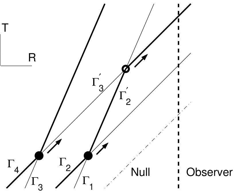
Figure 2: Emission from collisions. Trajectories: shells ejected from the central engine with hight Lorentz factor (thick solid), ones ejected with low Lorentz factor (thin solid) and observer (dashed). Collisions (circles) produce pulses of photons (arrows). The dashed dotted line shows the null geodesic passing through the central engine at $T=0$.

We here consider a evolution of four shells which is a basic component in multiple shell interaction. Since the observations require that shell widths should be much smaller than the separations, we assume infinitesimally thin shells for simplicity. We assign an index $i$, ($i=1,4$) to each shell according to the order of the emission from the central engine (see figure 2). The central engine ejects each shell with a Lorentz factor $\Gamma_{i}\gg 1$ at time $T_{i}$. We choose the origin of time such that the first shell is emitted at $T_{1}=0$. For convenience we define $D_{i}\equiv c\left(T_{i}-T_{i-1}\right)$ as the separation between shell $i-1$ and shell $i$.

To evaluate the conversion efficiency or the temporal properties of the internal shock process, it is important to understand how high velocity shells interact with slower ones and dissipate kinetic energy. Thus, we consider a case that the Lorentz factors of the shell 2 and the shell 4 are much higher than those of the shell 1 and the shell 3 $\Gamma_{2},\Gamma_{4}\gg\Gamma_{1},\Gamma_{3}$. The collision between the shell 1 and the shell 2 takes place at time $T\sim T_{2}+2\Gamma_{1}^{2}D_{2}/c$ and radius $R\sim 2\Gamma_{1}^{2}D_{2}$. The gamma-ray pulse produced by this collision arrives at the observer at the observer time $t=T-R/c\sim T_{2}+o(\Gamma_{1}^{2}/\Gamma_{2}^{2})$. We chose the origin of the observer time such that if a pulse was emitted from the engine at $T=0$, it would arrive at the observer at $t=0$ (dashed dotted line in figure 2). The pulse produced by the collision between the shell 3 and the shell 4 comes to the observer at $t\sim T_{4}+o(\Gamma_{3}^{2}/\Gamma_{4}^{2})$.

The mergers (filled circles) spread and cause a subsequent collision (open circle). Using the Lorentz factor of the shell 2 and the shell 3 after the collisions $\Gamma_{2}^{\prime}$ and $\Gamma_{3}^{\prime}$, the arrival time of the pulse from the subsequent collision can be estimated as $t\sim T_{4}+o(\Gamma_{2}^{\prime 2}/\Gamma_{3}^{\prime 2})$. If $\Gamma_{2}^{\prime}/\Gamma_{3}^{\prime}\ll 1$, the pulses from the collisions between the shell 3 and the shell 4 and between the shell 2 and the shell 3 are observed almost at the same time. If $\Gamma_{2}^{\prime}\sim\Gamma_{3}^{\prime}$, the collision can produce only a weak and soft pulse, it does not contribute to the main feature of the GRB light curve. Therefore, we observe pulses arising from the collisions mostly according to the time when high velocity shells were emitted by the central engine.

5.3 Multiple-Shells

We consider a wind consisting of $N$ shells. Each shell is characterised by four variables: Lorentz factor $\Gamma_{i}$, mass $m_{i}$, width $d_{i}$ and the distance to the outer neighbour shell $D_{i}$. As we wrote in section 4, most observed pulses in GRB light curves rise more quickly than decay, this means that the widths are smaller than the separations. Since, in such a case, light curves are not sensitive to the distribution of widths, for simplicity the width is assumed to be constant $d=D_{min}$. Though we will show numerical results with various distributions of $\Gamma_{i}$, $m_{i}$ and $D_{i}$ later, we first consider simple distributions with which we can give simple arguments to understand the numerical results. We assume that the Lorentz factors and the separations are distributed uniformly in logarithmic spaces; between $\Gamma_{min}$ and $\Gamma_{max}$ and between $D_{min}$ and $D_{max}$, respectively. We assume that the shells have equal mass. The internal shock process becomes very efficient if shells have the same mass and if the dispersion of the initial Lorentz factors is large (Beloborodov 2000; Kobayashi and Sari 2001). The value of mass is normalised by using the isotropic explosion energy $E_{iso}(\theta)$ as $m=E_{iso}/\Sigma\Gamma_{i}c^{2}$.

Our key assumption is a correlation between the Lorentz factors and the opening angle: wider jets have lower Lorentz factors $\Gamma\propto\theta^{-\alpha}$. The observed wide jets with $\theta\sim 0.2$ also should have ultra-relativistic Lorentz factors to be optically thin to high energy photons, we assume $\Gamma_{max}(\theta)=\Gamma_{0}~{}(\theta/0.2)^{-\alpha}$ and $\Gamma_{0}=100$

The evolution of the system in time is basically the same as in KPS97, but the photospheric effect is considered. We follow the evolution of shells until there are no more collisions, i.e. until the shells are ordered by increasing values of the Lorentz factors. The numerical light curves in the 50 - 300 keV BATSE band are plotted in Figure 3a-c for a model with different opening angles $\theta=$ 0.2, 0.06 or 0.02. Since we have assumed $\alpha=1$, these correspond to $\Gamma_{max}=100,333$ and $1000$, respectively. $N=100,\Gamma_{max}/\Gamma_{min}=10,D_{min}/c=1$msec, $D_{max}/c=1$sec and $\epsilon_{e}=\epsilon_{B}=0.1$ were also assumed. As we expected, the temporal profiles are more variable for narrower jets with higher Lorentz factors.

The definition of variability by Fenimore & Ramirez-Ruiz (2000) and that by Reichart et al (2001) are slightly different, but both relate the variability to the square of the time history after removing low frequencies by smoothing. To evaluate the variability of numerical light curves, we use a simplified version of the Reichart et al. (2001) variability,

$$V=\frac{\Sigma\left(C_{i}-\left\langle C\right\rangle\right)^{2}}{\Sigma C_{i}^{2}}$$ (6)

where $C_{i}$ is 50-300 keV photon counts at time $t_{i}$ with 64 msec resolution (the BATSE resolution), and $\left\langle C\right\rangle$ is the counts smoothed with a boxcar window with a time scale equal to the smallest fraction of the burst time history that contains a fraction $f$ of the total counts. Reichart et al. (2001) found that $f=45\%$ gives a robust definition of variability. Using the formula (6) with $f=0.45$, we evaluated the variability measures as $V=0.06,0.10$ and $0.25$ for Figure 3a, 3b and 3c, respectively.

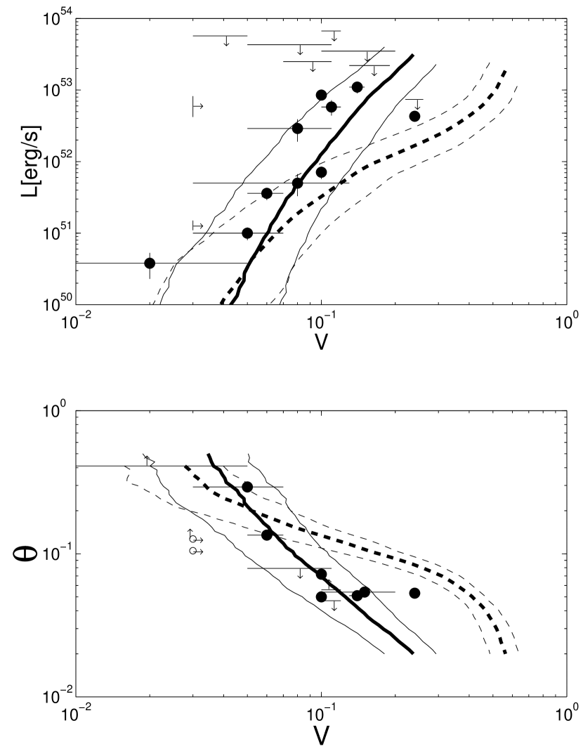
Figure 4: (a) Peak Luminosity vs. Variability with 1 $\sigma$ error bars of 100 random simulations. Observational data: measurements (filled circles) and upper or lower limits (arrows) are shown from Reichart et al (2001) and Frail et al (2001). $\alpha=1$(solid line), $\alpha=2$(dashed line) (b) Opening angles vs. Variability

Reichart et al (2001) found that the isotropic peak luminosities $L$ are correlated with the variability measures, $L\propto V^{3.3^{+1.1}_{-0.9}}$. We now show that such a correlation exists in our numerical simulations also. A numerical temporal profile depends on the specific realizations of random variables that are assigned to each shell, e.g. random Lorentz factors and random separations, as well as on the model parameters. For a given $\theta$ and the same model parameters as in Figure 3, we calculate the temporal profiles for 100 realizations, and evaluate the mean isotropic peak luminosity and the mean variability measure. Here the peak luminosity is calculated with 1 sec resolution as Reichart et al (2001) had analysed. In Figure 4a, the thick solid line shows the mean values, while the thin solid lines depict the 1$\sigma$ error. We also plot the opening angle-variability relation in Figure 4b. The numerical results reasonably fit the observational data, and can be understood using the following arguments.

5.4 Analytic Estimate

Numerous collisions happen during an evolution of multiple-shells. Each collision produces a pulse. However, the main pulses are produced by collisions between the fastest shells $\sim\Gamma_{max}$ and the slowest shells $\sim\Gamma_{min}$. Since such a collision happens at $R\sim\Gamma_{min}^{2}D_{i}$ for an initial separation $D_{i}$, we can define two characteristic collision radii, $\Gamma_{min}^{2}D_{min}$ and $\Gamma_{min}^{2}D_{max}$. In this equal mass case, mass is given by $mc^{2}\sim 2E_{iso}/N\Gamma_{max}$. The internal energy produced by a main collision and the Lorentz factor of the merger are $E_{int}\sim E_{iso}/N$ and $\Gamma_{m}\sim\sqrt{\Gamma_{max}\Gamma_{min}}$, respectively. The Thomson photosphere radius due to $e^{\pm}$ pairs from pair production interaction of synchrotron photons can be estimated by assuming that a significant fraction $\sim 10\%$ of the radiative energy $\epsilon_{e}E_{int}$ is converted to pairs.

$$R_{\pm} \sim \sqrt{\frac{\sigma_{T}\epsilon_{e}E_{iso}}{40\pi m_{e}c^{2}N\Gamma_{max}^{1/2}\Gamma_{min}^{1/2}}}$$ (7)

$$\sim 5\times 10^{14}~{}\mbox{cm}~{}E_{52}^{1/2}N_{2}^{-1/2}\Gamma_{0,2}^{-1/2}(\theta/0.2)^{-1/2},$$ (8)

hereafter $\epsilon_{e}=0.1$ is assumed.

If $R_{\pm}>\Gamma_{min}^{2}D_{max}$, the first collisions for most shells occur below the photosphere. However, since the shells reflect each other with the same velocity, it is still possible to produce bright pulses when the shells propagate beyond the photosphere and collide into other shells. If an enormous number of collisions and reflections happen below the photosphere, the shells are ordered with increasing values of the Lorentz factors and no collision happens any more. In order to produce bright pulses, the shells should come out from the photosphere before the slowest shells are sorted out at the tail of the wind with a total width $\Delta\sim ND_{max}/2$.

The equalities, $R_{\pm}=\Gamma_{min}^{2}D_{min}$ and $R_{\pm}=\Gamma_{min}^{2}\Delta$ give two opening angles.

$$\theta_{1} \sim 10^{-4}~{}E_{52}^{-1/3}N_{2}^{1/3}\Gamma_{0,2}^{5/3}D_{min,-3}^{2/3}$$ (9)

$$\theta_{2} \sim 10^{-1}~{}E_{52}^{-1/3}N_{2}\Gamma_{0,2}^{5/3}D_{max,0}^{2/3}$$ (10)

where $D_{min,-3}=(D_{min}/c)/10^{-3}$sec and $D_{max,0}=(D_{max}/c)/1$sec. Using these opening angles, GRBs are classified into the following three cases. (1) Narrow Jet Case: $\theta<\theta_{1}$. Since all collisions occur above the photosphere, the variability should be less dependent on $\theta$ and only on the distribution of the separations at the central engine. (2) Intermediate Jet Case: $\theta_{1}<\theta<\theta_{2}$. The variability of the temporal profile should highly depend on $\theta$. Some of the main collisions occur above the photosphere to produce bright pulses wider than

$$\delta t\sim R_{\pm}/2c\Gamma_{min}^{2}\sim 10^{-1}\mbox{sec}~{}E_{52}^{1/2}N_{2}^{-1/2}\Gamma_{0,2}^{-5/2}(\theta/10^{-2})^{3/2}.$$ (11)

(3) Wide Jet Case: $\theta>\theta_{2}$. The slowest shells are sorted out at the tail of the wind within the photosphere, only minor collisions happen. The resulting bursts become dimer.

Figure 3a is an example of the Wide Jet Case, while figure 3b and 3c correspond to the Intermediate Jet Case. Equation (11) gives rough estimates on the widths of main pulses for these Intermediate Jet Cases, $\delta t\sim 3$ sec $(\theta=0.06)$ and $\sim 0.5$ sec ($\theta=0.02$). Main pulses are actually wider in figure 3b. From figure 4b, the variability (thick solid line) is about $0.08$ at $\theta=\theta_{2}\sim 0.1$. In figure 4a, a linear fit to the numerical data for $V>0.08$ is $L\propto V^{3.8}$, which is consistent with a power law reported by Fenimore&Ramirez-Ruiz(2000) and by Reichart et al. (2001). Since the shells are ordered by velocity within the photosphere, the numerical luminosity rapidly decreases for $V<0.08$.

6 Other Initial Conditions

In our numerical simulation, we have assumed that a wider jet has a lower Lorentz factor $\Gamma\propto\theta^{-\alpha}$. A second assumption is that the shells have equal mass. A third concerns the distributions of the initial separations and the initial Lorentz factors. In this section, we discuss how numerical results depend on these assumptions.

Since the dynamics of the blast wave is determined only by two parameters: isotropic explosion energy and ambient matter density, afterglow emission does not depend on the initial Lorentz factor. The current afterglow observations detect radiation from several hours after the bursts. At this stage, the Lorentz factor of the blast wave is less than $\sim 10$. Then, the initial Lorentz factor can not be directly constrained through afterglow modelling. However, the Lorentz factor at the beginning of the afterglow stage can be estimated if one knows when the afterglow began.

An optical flash was observed during an exceptionally bright burst GRB990123, by using this peak time, the Lorentz factor was estimated as about 300 (Sari & Piran 1999; Kobayashi 2000). However, the optical flash was detected only for it so far. Panaitescu and Kumar (2002) assumed that the observed GRB duration is a good measure of the peak time, and found a correlation $\Gamma\propto\theta^{-0.3}$ within ten events for which opening angles are well constrained from the afterglow break time. Salmonson and Galama (2002) also have recently suggested the anticorrelation of $\Gamma$ with $\theta$, based on the positive correlation they observed in several cases between the GRB pulse lag time and the afterglow break time. However, the dependence they infer is much stronger $\Gamma\propto\theta^{-8/3}$. Therefore, we have done simulations with $\alpha=1/2$ and 2 also.

The numerical results with $\alpha=2$ are shown in figure 4a and 4b (dashed lines). The other parameters are the same with the case of $\alpha=1$ (solid line). For a larger value of $\alpha$, the Lorentz factor depends more strongly on the opening angle, while the photosphere radius becomes insensitive $R_{\pm}\propto\theta^{(\alpha-2)/2}$. Since the variability $V$ increases more rapidly with decreasing of the opening angle, the variability - luminosity relation becomes gentle. For $\alpha=1/2$, the numerical variability is insensitive to the opening angle. When we calculate $V$ in a range of $0.02<\theta<0.5$, it is almost constant $V\sim 0.05$. Therefore, the variability - luminosity relation becomes very steep. The numerical results with $\alpha\sim 1$ give the best fit to the observations. The mass loading at the central engine is $M\sim E/c^{2}\Gamma\propto\theta$, which is in a good agreement with a correlation $M\propto\theta^{1.1}$ reported by Panaitescu and Kumar (2002).

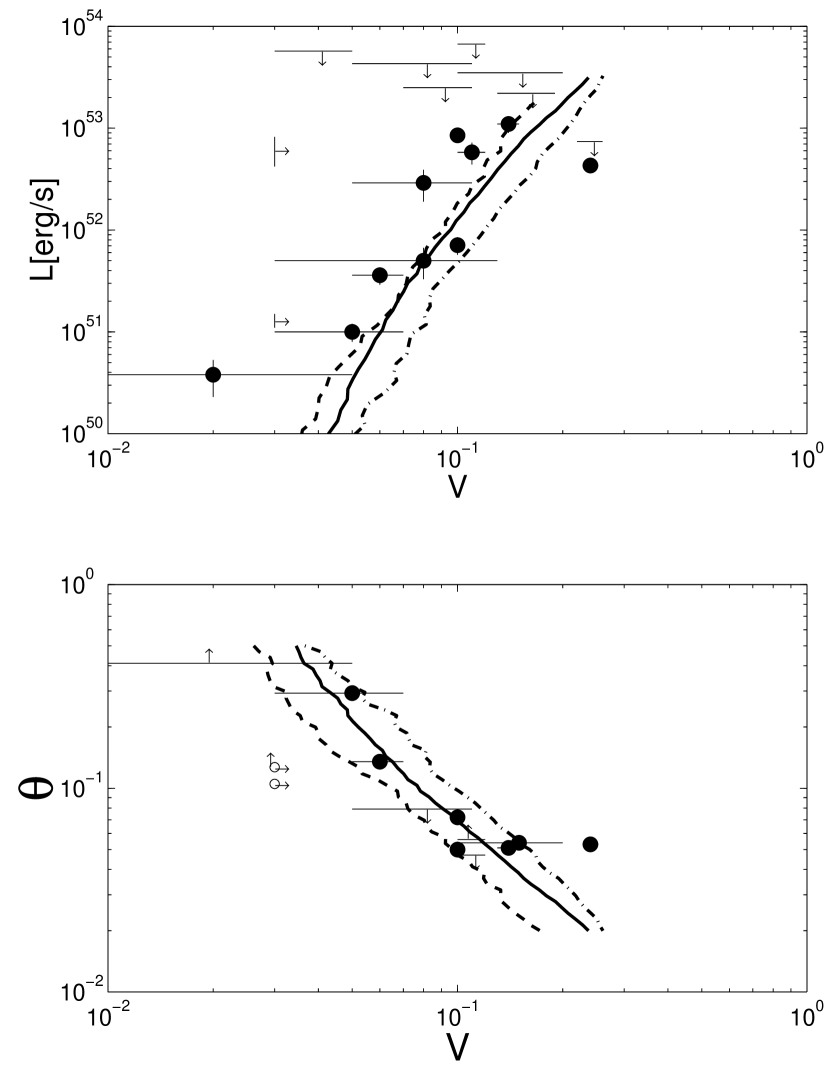
Figure 5: (a) Peak Luminosity vs. Variability : mean of 100 random simulations. Equal mass (solid line), equal energy (dashed line) and random mass (dashed dotted line). The parameters are the same with Figure 4($\alpha=1$) except the mass conditions. (b) Opening angles vs. Variability

We next discuss the assumption about mass. We also studied the cases that the shells have the same energy initially or have random masses. The random masses are assumed to be uniformly distributed between $m$ and $10m$. The value of $m$ is normalised at the beginning of the computation by the isotropic energy $E_{iso}=\Sigma m_{i}c^{2}\Gamma_{i}$. Under these mass assumptions, we calculate the temporal profiles for 100 realizations, and evaluate the mean isotropic peak luminosity and the mean variability measure. Figure 5a and 5b present the variability - luminosity and variability - opening angle relations. The equal energy (dashed line) and random mass (dashed dotted line) cases give similar results to the equal mass case (solid line). For a given $\theta$, the variability in the random mass case is larger than in the equal mass case. However, by choosing a smaller normalization of Lorentz factor $\Gamma_{0}\sim 80$, we can shift the line horizontally, and can get a more similar relation. Therefore, the equal mass assumption is not essential to get the observed correlation.

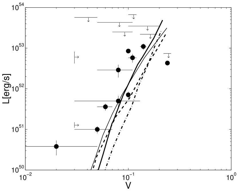
Figure 6: (a) Peak Luminosity vs. Variability : mean of 100 random simulations. Lognormal random intervals (thick solid). $\Gamma_{max}/\Gamma_{min}=100$ (dashed dotted) and Gaussian random Lorentz factors (dashed). $\Gamma_{max}/\Gamma_{min}=10$, uniform distributions of intervals and Lorentz factors are assume if the value or the distributions are not specified. $\alpha=1$ and equal mass are assumed in all cases. The thin solid line depicts the standard case.

GRB light curves contain many pulses with widths of msec to sec time scales. Since widths are determined by the initial separations, we considered a simple case that the initial separations $D_{i}$ are uniformly distributed in logarithmic spaces between $1$ msec and $1$sec. However, it is known that pulse widths have a lognormal distribution (Nakar & Piran 2001). We here consider a lognormal random intervals: a mean $\langle\log_{10}(D)\rangle=-2$ and a dispersion $\delta(\log_{10}(D))=1$. The thick solid line in figure 6 shows the numerical results, and is similar to the case of uniform distribution (thin solid line).

In order to achieve a high conversion efficiency $(>\mbox{a few}\%)$ from the explosion energy to gamma-ray in the internal shock process $\Gamma_{max}/\Gamma_{min}$ should be larger than $\sim 10$ (Kobayashi & Sari 2001). The dashed dotted line in figure 6 depicts the case of $\Gamma_{max}/\Gamma_{min}=100$, which steepness is comparable to the case of $\Gamma_{max}/\Gamma_{min}=10$ (thin solid). For a given luminosity, the variability is larger in this case. However, by using a smaller $\Gamma_{0}$, we can get a better fit to the observations. We also have done numerical simulations with a Gaussian random Lorentz factors where a mean value $\langle\Gamma\rangle=50(\theta/0.2)^{-1}$ and a dispersion $\delta\Gamma=\langle\Gamma\rangle$ are assumed. We truncated the initial Lorentz factor distribution for $\Gamma<2$, e.g. when we assign a random value to each shell at the beginning, random Lorentz factors are generated until $\Gamma_{i}>2$ is satisfied. The numerical results (dashed line) are also similar to the other cases (see figure 6).

We have shown that the variability - luminosity relation exists even if we make different assumptions on the distributions of masses, intervals and Lorentz factors and that the index and the normalization of the variability - luminosity relation highly depends on $\alpha$ and $\Gamma_{0}$. Our numerical results suggest $\alpha\sim 1$ and $\Gamma_{0}\sim 10^{2}$.

Another assumption concerns the values of $\epsilon_{e}$ and $\epsilon_{B}$, fractions of internal energy distributed to electrons and magnetic field at collisions. We have done another set of simulations with $\epsilon_{e}=\epsilon_{B}=0.3$ and get very similar results.

7 Conclusions

We have shown that there exists a correlation between the jet opening angle $\theta$ and the gamma-ray light curve variability $V$. Though the correlation is based on only seven events at present and needs to be further confirmed with more events, it is naturally expected if the luminosity $L$ is correlated with the variability (Fenimore & Ramirez-Ruiz 2000; Reichart et al. 2001), and if GRBs have a standard energy output (Frail et al. 2001; Panaitescu & Kumar 2002; Piran et al. 2001). This correlation might give us a way to measure the opening angle for a long burst directly from the GRB light curve.

We have shown that the opening angle - variability relation, or equivalently, due to the constancy of burst energy, the luminosity - variability relation can be interpreted as the correlation between the opening angle of a fireball jet and the Lorentz factor. Larger opening angles are expected to be associated with greater mass loading at the central engine and might result in lower Lorentz factors. We also show that such a correlation can be a natural consequence of the collapsar model. Using a multiple-shell model, we numerically calculate the temporal profiles and estimate the luminosity and the variability. Our numerical results suggest $\Gamma\propto\theta^{-1}$ or equivalently $M\propto\theta$.

If the opening angle of a jet is very wide $\theta\gg\theta_{2}$, the shells are almost ordered by increasing values of the Lorentz factors in the photosphere, only minor collisions or, at the extreme, only external shocks happen. The resulting dim burst should be smooth and has a soft spectrum. GRB980425 and recently reported Fast X-ray Transients (Heise et al. 2001; Kippen et al 2001) could be classified into this “Wide Jet Case”.

Norris, Marani & Bonnell (2000) found that the luminosity $L$ is inversely proportional to the GRB pulse lag time. The detailed study on the lag time is beyond the scope of this paper. However, if the time lag is also determined by the angular spreading time scale, which is the key time scale in our model, we can get the same relation. In our model, luminosity is scaled by the opening angle $L\propto\theta^{-2}$, while the angular spreading time is $t_{ang}\propto\Gamma^{-2}\propto\theta^{2}$. Then, we obtain $L\propto t_{ang}^{-1}$.

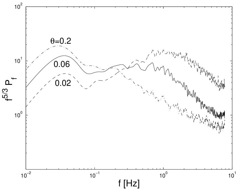
Figure 7: The averaged PDS for 100 random realizations. opening angle $\theta=0.2$(dashed dotted), 0.06 (solid) and 0.02 (dashed). The initial parameters are the same as in Fig 3

Another measure of variability in light curves is the power density spectra (PDSs). The observed PDSs show a strong correlation with the luminosity (Beloborodov, Stern and Svensson 2000). In each case of figure 3 a, b and c, we calculate the light curves for 100 realizations, and evaluate the average PDS $P_{f}$. The averaging means that we sum up the PDSs of the numerical profiles with the peak normalisation, and divided by the number of realizations, 100. The numerical PDSs show a strong correlation with the opening angles : brighter bursts with smaller opening angles have more variable power at high frequency (see figure 7). It resembles the results for different brightness classes of real bursts (figure 8 in Beloborodov, Stern and Svensson 2000). The numerical results reproduce the slope index of $\sim-5/3$ and the 1 Hz break also which Beloborodov, Stern and Svensson (2000) found in observed light curves. The photosphere radius $R_{\pm}$ is about $5\times 10^{14}$ cm and weakly depends on parameters. The collisions which produce 1sec pulses happen around a radius $\sim 6\times 10^{14}(\Gamma_{min}/100)^{2}$ cm. If $\Gamma_{min}\sim 100$, the 1Hz break can be explained by the phtospheric effect. The constraints on the activity of the central engine from the PDS study will be discussed in the subsequent paper.

In our model, more variable bursts have higher Lorentz factors, and therefore are expected to have higher spectral peak energy. We can actually see such a trend in the observational data when correcting the cosmological expansion effect(Table 1 of Fenimore and Ramirez-Ruiz 2000). Ramirez-Ruiz and Lloyd-Ronning (2002) recently extended our study to examine the spectral property of GRBs. Their numerical results reproduce the trend.

Most studies on GRBs assume a jet with a well-defined angle, though this angle differs for different bursts. However, Rossi, Lazzati & Rees (2001) and Zhang & Mészáros (2001) proposed an alternative model where the jet, rather than having a uniform profile out to some definite cone angle, has a beam pattern. Even in this model, the more luminous part of a jet has a higher Lorentz factor. Then, our results can be applied to explain the variability - luminosity relation.

We would like to thank the Aspen Center for Physics for their hospitality and for providing a pleasant working environment where this work was initiated. We would also like to thank Nicole M. Lloyd-Ronning for useful discussions. We thank the anonymous referee for valuable suggestions that enhanced this paper. S.K. acknowledges support from the Japan Society for the Promotion of Science. F.R. acknowledges support from the Swedish Foundation for International Cooperation in Research and Higher Education (STINT). A.M. acknowledges support from DOE ASCI (B347885).

References
Asano,K., & Kobayashi, S. 2002, in preparation.
Beloborodov,A.M. 2000, ApJ, 539, L25.
Beloborodov,A.M., Stern,B.E. & Svensson,R. 2000, ApJ, 535, 158.
Fenimore,E., & Ramirez-Ruiz, E. 2000, Submitted to ApJ, (astro-ph/0004176).
Frail, D. A., et al. 2001, ApJ, 562, L55.
Guetta,D., Spada,M., & Waxman E. 2001, ApJ, 557,399.
Heise, J., et al. 2001, Proc. Second Rome Workshop
Kippen, R. M., et al. 2001, Proc. Second Rome Workshop, astro-ph/0102277.
Kobayashi,S. 2000, ApJ, 545, 807.
Kobayashi,S., Piran,T. & Sari,R. 1997, ApJ, 490, 92.
Kobayashi,S., Piran,T. & Sari,R. 1999, ApJ, 513, 669.
Kobayashi,S., & Sari,R. 2001, ApJ, 542, 819.
Lloyd-Ronning,N.M., Fryer,C.L & Ramirez-Ruiz,E. 2001, ApJ in press.
MacFadyen,A. & Woosley,S. 1999, ApJ, 524, 262.
Mészáros, P., & Rees,M.J. 2000 ApJ, 530, 292.
Nakar,E., & Piran,T. 2001, MNRSA in press (astro-ph/0103210).
Narayan, R., Piran, T. &Kumar, P., ApJ 557, 949.
Norris, J.P. et al. 1996, ApJ, 459, 393.
Norris, J.P., Marani,G.F., & Bonnell,J.T. 2000, ApJ, 534, 248.
Panaitescu,P. & Kumar,P. 2002, ApJ in press (astro-ph/0109124).
Piran,T., 2000, Phys. Rep., 333, 529.
Piran,T., et al. 2001, ApJL in press (astro-ph/0108033).
Ramirez-Ruiz, E. & Lloyd-Ronning, N.M. 2002, New Astronomy in press.
Ramirez-Ruiz, E. & Fenimore,E. 1999, Presentation at the 1999 Huntsville GRB conference.
Rossi,E., Lazzati,D. & Rees,M.J. 2002, MNRAS in press.
Reichart,D. E., et al. 2001, ApJ, 552, 57.
Ryde,F., & Petrosian,V. 2002, in preparation.
Salmonson,J.D. & Galama,T.J. 2002, ApJ in press (astro-ph/0112298).
Sari,R., Narayan, R., & Piran,T. 1996, ApJL, 473, 204.
Sari,R. & Piran,T. 1999, ApJL, 517, 109.
Stern,B., Poutanen,J. & Svensson,R. 1999, ApJ, 510, 312.
Woosley,S. 1993, ApJ 405, 273.
Zhang,B. & Mészáros,P. 2002, ApJ in press (astro-ph/0112118).
Zhang,W, Woosley, S., & MacFadyen, A. 2002, in preparation.

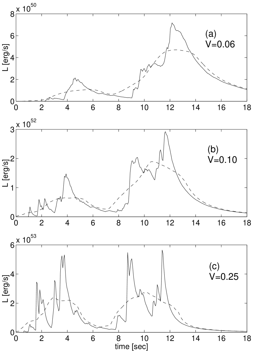
Figure 3: Temporal structures (50-300 keV) for different opening angles. (a) $\theta=0.2$. (b) $\theta=0.06$. (c) $\theta=0.02$. The dashed lines show the structures smoothed with the boxcar wind.