MODELS FOR THE UV-X EMISSION IN AGN: INFLUENCE OF DIFFERENT PARAMETERS

Abstract

We present the results of computations performed with a new photoionisation-transfer code designed for hot Compton thick media. Presently the code solves the transfer of the continuum with the Accelerated Lambda Iteration method (ALI) and that of the lines in a two stream Eddington approximation, without using the local escape probability formalism to approximate the line transfer. We show the influence that the approximations made in the treatment of the transfer and of the atomic data can have on the broad band UV-X spectrum and on the detailed spectral features (X-ray lines and ionization edges) emitted/absorbed by an X-ray irradiated medium. This transfer code is coupled with a Monte Carlo code which allows to take into account direct and inverse Compton diffusions, and to compute the spectrum emitted up to hundreds of keV energies. The influence of a few physical parameters is shown, and the importance of the density and pressure distribution (constant density, pressure equilibrium) is discussed.

1 The codes

Using a photoionisation-transfer code specially designed for hot Compton thick media ($T\geq 10^{4}K$, Thomson depth $\tau_{es}$ can be as large as a few hundreds), we are able to compute the thermal and ionisation structure and the spectrum emitted and reflected by a slab of gas illuminated on one side or on both sides by a given spectrum in a plane-parallel geometry (for a description of the code, see Dumont et al.  [1] and Dumont & Collin  [2]). Contrary to the other photoionisation codes which use the escape probability (EP) formalism, our code solves the transfer of the continuum with the Accelerated Lambda Iteration (ALI) procedure and that of the lines with a two stream approximation (ALI is being implemented presently for the lines). It is coupled with a Monte-Carlo code which allows to take into account Compton and inverse Compton diffusions, and to compute the spectrum emitted up to hundreds of keV energies, in any geometry.

The gas composition includes 10 elements and 102 ions. H is treated as a 6-level atom, H-like and Li-like as 5-level atoms, He-like ions as 8-levels atoms and matrix inversions are performed to compute the levels populations. The other ions are treated roughly as two level atoms plus a continuum. All collisional and radiative processes (including ionizations from and recombinations onto excited levels) are taken into account. Recombinations onto upper levels ($n>6$ for H, $n>5$ for H- and Li-like ions, $n>8$ for He-like ions) are added to our highest excited level.

2 Results

We consider here two cases :

• the density is constant across the slab

• the pressure is constant across the slab

In the present examples the incident continuum is a power law with a slope of unity (in flux, $F_{\nu}$) from 0.1 eV to 100 keV. We take cosmic abundances. The density at the surface of the slab is $10^{12}$cm^-3 and the incident flux is equal to $8\ 10^{13}$ erg cm^-3 s^-1 (corresponding to an ionisation parameter $\xi=L/(n_{H}R^{2})=1000$ erg.cm.s^-1) in constant pressure and constant density cases.

2.1 Influence of the transfer treatment

In Dumont et al.  [1], it was shown that the neglect of the returning radiation often used in photoionisation codes, i.e. the “outward only” approximation, leads to strong temperature errors, in particular at the illuminated face of the slab when the slab is thick ($\tau_{es}\geq 0.1$).

One other difference between EP and transfer lies in the fact that the line emissivity can be negative whereas it is impossible in EP (see  [1]). This translates into a difference in the energy balance, which can have important consequences on the equilibrium temperature (see Fig. 1 for an example in the constant pressure case).

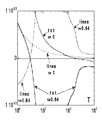
Figure 1: Radiative rate cooling-heating curves (full lines) and net cooling curves due to lines (dashed lines) for different optical thicknesses in the constant pressure case ($\tau_{es}=0$ and equilibrium temperature $T_{eq}=2\ 10^{6}K$, $\tau_{es}=0.64$ and $T_{eq}=3.5\ 10^{4}K$). One can see that the line cooling which dominates the energy balance becomes negative close to the equilibrium temperature.

2.2 Influence of the atomic data

The model atoms are important not only for the thermal balance, but also for the ionization equilibrium. Fig. 2 shows the temperature profile and Fig. 3 the fractional abundances of oxygen versus optical thickness, for two different treatments of the atomic data, in the constant density case. When only H-like ions are treated with multi-level atoms, the temperature is higher than in the treatment with H-like, He-like and Li-like multi-level ions for an optical thickness smaller than about 2 and then is lower, for larger optical thicknesses.

Treating H-, He-, Li-like ions as multi-level atoms produce more lines than with only H-like multi-level atoms; all these added lines cool the medium which leads to a cooler temperature in the case of H-, He-, Li-like multi-level ions. The temperature profile declines faster in the H-like description than in the ’total’ description between $\tau_{es}=2$ and $\tau_{es}=3$ because in that place, photoionization from the excited levels of Li-like ions are as important as those from the ground level in contradistinction to H-like and He-like ions where the photoionisation from excited levels is always negligible. When looking at the fractional abundances of oxygen, one sees that O VIII is present deeper in the cloud in the description with H-, He-, Li-like multi level atoms than in the treatment with only H-like multi level atoms. This is due to an approximate treatment of losses due to recombination radiation in the two-level atoms.

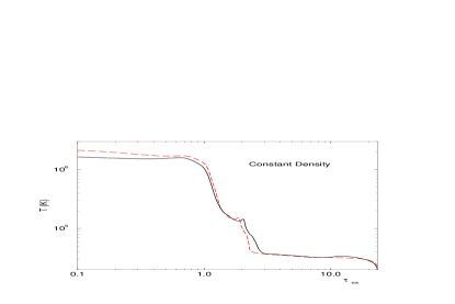
Figure 2: Temperature profile versus optical thickness, for a treatment with only multi-level H-like ions (dashed lines), and with H-like, He-like and Li-like multi-level ions (full lines) for a constant density model.

Figure 3: Fractional abundances of oxygen versus optical thickness for the same two treatments of the atomic data. As in Fig. 2, the example shown here is for a constant density model.

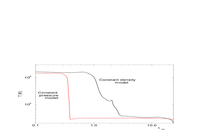
Figure 4: Temperature profile versus optical thickness for the constant density and the constant pressure cases. The temperature decreases abruptly in the constant pressure case, when the soft X-ray photons are absorbed.

Figure 5: Fractional abundances of oxygen versus optical thickness for the constant pressure case. Note that, in the constant density case (fig 3), only highly ionized species are present in the regions contributing to the emission, while in the constant pressure case, both high and low ionization species are present.

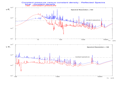
Figure 6: Comparison of the reflected spectrum between 1 eV and 25 keV in a constant density and a constant pressure cases.

2.3 Comparison of constant density and constant pressure models

The slab being illuminated with the same irradiating flux, we compare the results in the constant density and in the constant pressure cases. The temperature profiles and fractional abundances of oxygen are shown on Figs. 2, 4 and  3, 5 respectively. At first sight, one sees that the thermal and ionization structure are completely different in the two different cases, owing to the phase change of the photoionized gas in the constant pressure case (see Krolik et al.  [3]) when soft X-ray photons have been absorbed. The temperature decreases abruptly and consequently the density increases in the constant presssure case. Accordingly, the emission-reflection spectra are different. Fig. 6 shows the reflected spectra in the constant density and the constant pressure cases, and Fig. 7 is a zoom of Fig. 6 between 0.1 and 20 keV on which a few lines and edges are identified. Some line equivalent widths (EWs) of interest, in the constant density and constant pressure cases, are given in Table  1. We recall that the EWs are those measured only on the reflected spectra with no dilution due to the incident spectrum.

Due to the absence of layers with an intermediate temperature in the constant pressure case, the “intermediate” ions are almost absent. As a consequence, the iron lines correspond to both high and low ionization species, in contradistinction to the constant density case. Finally, due to the absence of intermediate temperature layers giving rise to soft X-ray reflection, the reflected spectrum in the constant pressure case displays a narrower “Blue Bump” than in the constant density case.

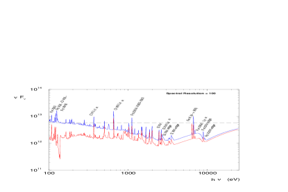
Figure 7: Zoom of Fig. 6 between 100 eV and 20 keV. A few lines and edges are labelled in the figure, but others are identified in Table  1.

3 Foreseen improvements

Presently we are implementing the ALI method in the transfer of the lines which are the most difficult to converge.

We intend to treat all ions as multi-level atoms and to add levels to those already treated like this. We will take into account some forbidden lines which could be important for the cooling of the medium in some places.

Though there are still many improvements to perform, we already use theses codes to describe AGN spectra in the UV and X-ray range, in their validity range. In particular, the code is used to compute the spectrum emitted by an irradiated slab in hydrostatic equilibrium (see Różańska et al. in this workshop).

Table 1: Measured Equivalent Widths (reflected spectra)

Ion	$h\nu$(eV)	EWa(eV)	EWb(eV)
Fe XXVI $Ly\alpha$	6957.7	28.06	17.15
Fe XXV	6667.7	237.7	145.6
Fe K $(V\rightarrow XIV)$	6400.0	6.362	180.6
S XVI	3342.8	4.594	6.056
S XVI $Ly\alpha$	2611.3	42.90	47.16
S XV	2450.3	32.28	42.51
Si XIV $Ly\alpha$	1999.8	27.18	30.67
Si XII	1865.0	4.892	7.637
Fe XXIV	1673.2	27.44	21.00
Fe XXIV	1495.6	16.01	10.57
Mg XI	1343.3	6.034	11.19
Fe XXII-XXIII	1127.1	3.698	6.986
Fe XXIV	1110.0	35.03	26.44
Ne X $Ly\alpha$	1020.3	13.46	16.30
Fe XVII	821.10	4.957	4.025
Fe VII	729.33	1.951	2.978
O VIII $Ly\alpha$	653.35	26.37	32.75
Fe XXIV	563.57	2.466	2.001
N VII $Ly\alpha$	500.14	3.895	5.429
C VI $Ly\alpha$	367.36	5.263	9.009
Mg X	194.61	1.079	0.468
O VIII	163.33	0.744	1.360
Fe XVIII	127.82	0.285	1.578
O VIII	120.98	1.577	2.706
Fe XIX	118.08	0.711	2.327
Fe XXII	107.81	0.878	3.376
a constant density case
b constant pressure case.

References

- [1] Dumont, A.-M., Abrassart, A., & Collin, S. 2000, A&A, 357, 823
- [2] Dumont, A.-M., & Collin, S. 2001, ASP Conf. Series, vol XXX, Gary Ferland & Daniel Wolf Savin, eds
- [3] Krolik, J.H., McKee, C.F., & Tarter, C.B. 1981, ApJ, 249, 422