Cosmic Shear from STIS Pure Parallels
II Analysis

1 Cosmic Shear

The measurement of cosmic shear requires deep imaging (to beat the noise due to the galaxies’ intrinsic ellipticity distribution) with high image quality (because every non-corrected PSF anisotropy mimics cosmic shear) on many lines of sight to sample the statistics of large-scale structure. The STIS camera on-board HST has a very good performance in that respect, which we demonstrate here, by using archival data from the STIS pure parallel program between June 1997 and October 1998. The data reduction and catalog production are described in the poster Detection of Cosmic Shear From STIS Parallel Archive Data: Data Analysis presented here and the paper Pirzkal et al. (2001).

2 STIS: PSF correction

The expected distortion of galaxy images by cosmic shear on the angular scale of STIS ($\sim 50^{\prime\prime}$) is a few percent, therefore the PSF anisotropy has to be understood and controlled to an accuracy of better than 1%. In Fig. 1 we show that the mean ellipticity of stars are small and can be considered constant at the one sigma level.

Figure 1: Mean of the ellipticity $e_{1}$ (left) and $e_{2}$ (right) of the star fields vs. exposure start time (Modified Julian Date). Both components can be approximated by a constant over the time period covered. The staight lines show the mean over all the fields, the dashed lines are the corresponding $1\sigma$ errors. The circles denote the mean over stars in bins between $5.06\times 10^{4}$, $5.08\times 10^{4}$, $5.10\times 10^{4}$, $5.12\times 10^{4}$ (MJD) with the corresponding 1$\sigma$ error bars.

In addition to the variations from field to field, we find a spatial variation of the PSF within individual fields, as shown in Fig. 3, to which we fitted a second-order polynomial as a function of position on the CCD. We also find some very short timescale variations of the PSF (also shown in Fig. 3) which are likely due to breathing of the telescope.

In Fig. 2 we show that the PSF anisotropy corrections are very small, they change the mean of the galaxy ellipticities on a field only slightly. We also checked the effect of the anisotropy correction on the cosmic shear result and find that it does not change noticeably.

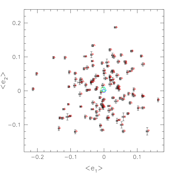
Figure 2: For 121 galaxy fields we plot the mean uncorrected ellipticity of galaxies (triangles) as well as the mean corrected ellipticity (squares). The error bars attached to the squares denote 3 times the dispersion of the field-averaged corrected ellipticities when the different PSF model fits are used. The shift of the corrected mean ellipticities towards negative $e_{1}$ is expected from the behaviour of the stellar ellipticities plotted in Fig. 1. The red triangle and cyan square in the center denote the mean over all galaxy fields of the uncorrected and corrected mean ellipticities, respectively; the size of the symbols show the $1\sigma$ errors on the mean. The circle shows the origin for reference. The mean is compatible with zero.

      

Figure 3: For one of the star fields the distribution of the ellipticities of stars are shown before (top left) and after (top right) correcting for PSF anisotropy. The middle left panel shows the spatial distribution of the ellipticities across the STIS field, the middle right the fitted second order polynomial at the star positions. The length of the sticks indicates the modulus of the ellipticity, the orientation gives the position angle. For individual exposures of this field, which were taken with a time difference of only 30 minutes we show the values of the polynomials for the anisotropy correction in the lower panels. One clearly sees the short timescale variations which are likely due to breathing of the telescope.

3 Results

We analysed the ellipticities of galaxies in 121 galaxy fields, which were corrected for PSF effects using 21 measured PSFs from low galactic latitude fields (star fields). The quantity estimated was the shear dispersion in each field. We apply a weighting to individual galaxies according to the weighting scheme in Erben et al. (2001). By randomizing the orientations of the galaxy images, we obtain probability distributions for our estimator in the absence of shear, which are shown in Fig. 4, with and without applying the weighting; this serves as an estimate of the significance of our result.

In Fig. 5 we compare our result for the cosmic shear with weighting individual galaxies to those obtained for larger scales by other groups.

Acknowledgements This work was supported by the TMR Network “Gravitational Lensing: New Constraints on Cosmology and the Distribution of Dark Matter” of the EC under contract No. ERBFMRX-CT97-0172 and by the German Ministry for Science and Education (BMBF) through the DLR under the project 50 OR106.

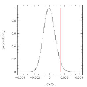
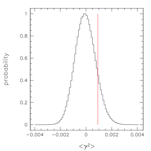
Figure 4: Probability distribution of the cosmic shear dispersion estimator calculated from the data by randomizing the orientations of galaxies. The vertical line indicates the actually measured value; left is with, right without weighting the galaxies depending on their noise level.

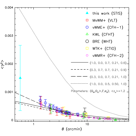
Figure 5: Comparison of our cosmic shear result (big triangle at $0.5^{\prime}$) with measurements at larger angular scales and with model predictions. The lines show the theoretical predictions if one uses different cosmological models, where we indicate $\Omega_{m}$, $\Omega_{\Lambda}$, $h$, $\Gamma$ and $\sigma_{8}$. The redshift distribution was taken from Brainard et al. (1996) with a mean source redshift of $\left\langle z_{\mathrm{s}}\right\rangle=1.2$. Given the different galaxy selection implied by our STIS data, which may imply a substantially different redshift distribution from that obtained from ground-based observations, the apparent discrepancy may be due to a higher mean redshift.

References


Bacon, D., Refregier, A., Ellis, R.S., 2000, MNRAS, 318, 625
Brainerd, T.G., Blandford, R.D., Smail, I., 1996, ApJ, 466, 623
Erben, T., van Waerbeke, L., Bertin, E., Mellier, Y., Schneider, P., 2001, A&A, 366, 717
Kaiser, N., Wilson, G., Luppino, G.A., 2000, submitted to ApJ, astro-ph/0003338
Maoli, R., Mellier, Y., van Waerbeke, L., Schneider, P., Jain, B., Bernardeau, F., Erben, T., Fort, B., 2001, A&A, 368, 766
Pirzkal, N., Collodel, L., Erben, T., Fosbury, R.A.E., Freudling, W., Hämmerle, H., Jain, B., Micol, A., Miralles, J.-M., Schneider, P. Seitz, S., White, S.D.M., 2001, A&A in press, astro-ph/0102330
van Waerbeke, L., Mellier, Y., Erben, T., Cuillandre, J.C., Bernardeau, F., Maoli, R., Bertin, E., Mc Cracken, H.J., Le Fèvre, O., Fort, B., Dantel-Fort, M., Jain, B., Schneider, P., 2000, A&A, 358, 30
van Waerbeke, L., Mellier, Y., Radovich, M., Bertin, E., Dantel-Fort, M., Mc Cracken, H.J., Le Fèvre, O., Foucaud, S., Cuillandre, J.C., Erben, T., Jain, B., Schneider, P., Bernardeau, F., Fort, B., 2001, A&A in press, astro-ph/0101511
Wittman, D.M., Tyson, J.A., Kirkman, D., Dell’Antonio, I., Bernstin, G., 2000, Nature, 405, 143