Formation and pre–MS evolution of massive stars with growing accretion

Abstract

We briefly describe the three existing scenarios for forming massive stars and emphasize that the arguments often used to reject the accretion scenario for massive stars are misleading. It is usually not accounted for the fact that the turbulent pressure associated to large turbulent velocities in clouds necessarily imply relatively high accretion rates for massive stars.

We show the basic difference between the formation of low and high mass stars based on the values of the free fall time and of the Kelvin-Helmoltz timescale, and define the concept of birthline for massive stars.

Due to D-burning, the radius and location of the birthline in the HR diagram, as well as the lifetimes are very sensitive to the accretion rate $\dot{M}_{\mathrm{accr}}$. If a form $\dot{M}_{\mathrm{accr}}\propto A\,(M/M_{\hbox{$\odot$}})^{\varphi}$ is adopted, the observations in the HR diagram and the lifetimes support a value of $A\approx 10^{-5}\,M_{\hbox{$\odot$}}\cdot{\mathrm{yr}}^{-1}$ and a value of $\varphi\mathrel{\hbox{\hbox to0.0pt{\hbox{\lower 4.0pt\hbox{$\sim$}}\hss}\hbox{$>$}}}1$. Remarkably, such a law is consistent with the relation found by Churchwell (1998) and Henning et al. (2000) between the outflow rates and the luminosities of ultra–compact HII regions, if we assume that a fraction $0.15$ to $0.3$ of the global inflow is accreted. The above relation implies high $\dot{M}_{\mathrm{accr}}\approx 10^{-3}\,M_{\hbox{$\odot$}}\cdot{\mathrm{yr}}^{-1}$ for the most massive stars. The physical possibility of such high $\dot{M}_{\mathrm{accr}}$ is supported by current numerical models.

Finally, we give simple analytical arguments in favour of the growth of $\dot{M}_{\mathrm{accr}}$ with the already accreted mass. We also suggest that due to Bondi-Hoyle accretion, the formation of binary stars is largely favoured among massive stars in the accretion scenario.

Geneva Observatory, CH-1290 Sauverny, Switzerland

1. Introduction

Numerous new observations in radio, IR, optical, UV and X–rays, together with many numerical models, have contributed to the progress of the field of star formation. However, the formation of massive stars is still a major unsolved problem in stellar evolution.

The answer brought to the question ”How do massive stars form ?” has a major impact not only for stellar evolution, but also for spectral and chemical evolution of galaxies as well as for cosmology. Several competing processes have now been identified leading to different scenarios for the formation of massive stars. Nevertheless, this does not mean that the authors of these scenarios are competing. Rather they all look for the proper answer to the above major question.

2. The various scenarios for the formation of massive stars

One can identify three different scenarios:

a) The classical scenario.
This is the pre–MS evolution at constant mass with bluewards horizontal tracks in the HR diagram, moving from the Hayashi line to the zero age main sequence (ZAMS), (cf. Iben 1963). The timescale is the Kelvin-Helmholtz timescale $t_{\mathrm{KH}}\approx G\,M^{2}/R\,L$ which is about 0.5 to 2% of the MS lifetime. For example, $t_{\mathrm{KH}}$ is about $3\cdot 10^{4}\,{\mathrm{yr}}$ for a $30\,M_{\hbox{$\odot$}}$ star. Due to lots of evidence of mass accretion (see below, § 3.), this scenario is no longer supported, although it is a good reference basis.

b) The collision or coalescence scenario.
Protostars are moving around in a young cluster and collisions of intermediate mass protostars may lead to the formation of massive stars. This interesting possibility and its consequences have been extensively studied by Bonnell, Zinnecker and colleagues (cf. Bonnell et al. 1998).

Often in the literature (cf. Stahler 1998), it is said that the coalescence scenario is necessary, on the basis of the argument that the accretion scenario is not possible for massive stars because their high radiation pressure on the dust may reverse the infall and prevent the accretion. We emphasize that the coalescence scenario may well be important, but not for this specific reason. The reasons are the following ones.

We may consider that the accretion rate $\dot{M}_{\mathrm{accr}}$ is given by

$$\dot{M}_{\mathrm{accr}}\approx c_{\mathrm{s}}{}^{3}/G$$ (1)

as resulting from the ratio of the Jeans mass by the free fall time. For typical temperatures of $10$-$100\,{\mathrm{K}}$, as observed in molecular clouds, a value of $\dot{M}_{\mathrm{accr}}\approx 10^{-5}\,M_{\hbox{$\odot$}}\cdot{\mathrm{yr}}^{-1}$ is obtained from relation (1). It is true that for such values of $\dot{M}_{\mathrm{accr}}$, the effects of the radiation pressure $P_{\mathrm{rad}}$ can reverse the infall. However, this argument ignores the role of turbulent pressure in the clouds. Indeed, high turbulent velocities have been observed in regions of massive stars (cf. Tatematsu et al. 1993; Caselli & Myers 1995; Nakano et al. 1995; Nakano et al. 2000). If we account for the turbulent velocities in equation (1), there is more support in the clouds which are thus denser and one gets much higher accretion rates of the order of

$$\dot{M}_{\mathrm{accr}}\approx 10^{-3}\,M_{\hbox{$\odot$}}\cdot{\mathrm{yr}}^{-1}.$$

For such a high accretion rate, the momentum of the infalling material is higher than the momentum in the outgoing radiation of a massive star and the accretion can not be reversed (see below, § 5.1.). Thus, the basic argument often used against the accretion scenario is invalid, since it does not account for the fact that the accretion rates are very high.

This does not mean that the coalescence scenario never works. But, one has to be careful about the question of its timescale. In particular Elmegreen (2000) has suggested that ”there is not enough time for a protostar to move around in a young cluster and to coalesce with other protostars”. Certainly collisions do occur, but the real importance of this scenario has still to be ascertain.

c) The accretion scenario.
The accretion scenario with constant $\dot{M}_{\mathrm{accr}}$ was first proposed by Beech & Mitalas (1994). It is however evident that with moderate accretion rate like $\dot{M}_{\mathrm{accr}}\approx 10^{-5}\,M_{\hbox{$\odot$}}\cdot{\mathrm{yr}}^{-1}$, we would need $10^{7}\,{\mathrm{yr}}$ to form a $100\,M_{\hbox{$\odot$}}$ star. At this age, it would already have exhausted its central hydrogen. Thus, one needs accretion rate growing with time or with the stellar mass (cf. Bernasconi & Maeder 1996; Norberg & Maeder 2000; Behrend & Maeder 2001; McKee, this meeting). The various properties of these models will be discussed in section 4..

3. Brief summary of the observational evidence for the formation of massive stars by accretion

As shown by several recent works as well as in this meeting, there are several observational indications in favour of the massive star formation by accretion.

• Massive outflows.

  There is evidence from radio observations of massive outflows (cf. Churchwell 1998; Henning et al. 2000) with outflow rates $\dot{M}_{\mathrm{accr}}\propto L^{0.75}$ where $L$ is an estimate of the stellar luminosity. A fraction $15\%$ to $30\%$ of the global infall is supposed to be accreted, while the rest goes into the outflows. This suggests that during the formation of massive stars, the accretion rate may grow relatively steeply with the already accreted stellar mass.

• Velocity dispersion.

  High velocity dispersions are observed, as for example from the CS line in the Orion KL Nebula (Caselli & Myers 1995). This supports the idea that turbulence provides enough support to the cloud to allow a high enough density, which then leads to accretion rates of the order of $10^{-3}\,M_{\hbox{$\odot$}}\cdot{\mathrm{yr}}^{-1}$.

• Luminosity.

  The luminosity of IR sources like the Orion IRC2 K–luminosity is quite compatible with luminosities of $L\propto{G\,M\,\dot{M}\over R}$ of discs having accretion rates of the order of $10^{-2}$ to $10^{-3}\,M_{\hbox{$\odot$}}\cdot{\mathrm{yr}}^{-1}$ (Morino et al. 1998; Nakano et al. 2000).

• Spectra.

  Also the spectral distribution of the energy emitted by hot cores in hot molecular clouds is compatible with discs having accretion rates as given above (Osorio et al. 1999).

• Direct evidence for discs.

  Direct evidence for discs has been provided. An example is IRAS 20126 +4004 from $\textrm{NH}_{3}$ line observed by the VLA (Zhang et al. 1998; Cesaroni 2000). The disc looks perpendicular to the molecular outflow, and a velocity gradient is observed in the disc. Further compelling evidence of discs has been presented at this meeting by Zhang and by Conti.

Interestingly enough, a prediction of the coalescence scenario is that discs should be destroyed by the collision, thus the visibility of discs may be an evidence against the coalescence.

4. The accretion scenario: semi-empirical approach

4.1. Generalities

We are using various approaches, here. The semi-empirical approach which gives rough overall constraints, the analytical one which emphasizes the relation between basic parameters, and the accurate numerical one (cf. § 5.2.).

There is a fundamental difference between low and high mass stars, from the point of view of star formation if we consider the free fall time

$$t_{\mathrm{ff}}={3\,\pi\over\sqrt{32\,G\,\bar{\rho}_{\mathrm{in}}}}$$ (2)

and the Kelvin-Helmoltz timescale

$$t_{\mathrm{KH}}={G\,M^{2}\over R\,L}\,,$$ (3)

where $\bar{\rho}_{\mathrm{in}}$ is the average initial density of the cloud supposed to be at Jeans limit (i.e. $R_{\mathrm{J}}\propto M_{\mathrm{J}})$. For $M\leq 8\,M_{\hbox{$\odot$}}$ (in the numerical model of Figure 1, this limit turns to be around $15\,M_{\odot}$), one has

$$t_{\mathrm{ff}}<t_{\mathrm{KH}}.$$

This means that the accretion process is completed long before the central contraction has initiated nuclear burning. Thus, in this range of masses, the evolution is not so far from the evolution at constant mass. For $M\mathrel{\hbox{\hbox to0.0pt{\hbox{\lower 4.0pt\hbox{$\sim$}}\hss}\hbox{$>$}}}8\,M_{\hbox{$\odot$}}$, one has

$$t_{\mathrm{ff}}>t_{\mathrm{KH}}.$$

In this case, the accretion is not yet completed when the central core has already finished its contraction and started nuclear burning. Thus, massive stars start their H-burning largely hidden in their molecular clouds, a fact consistent with the observations by Wood & Churchwell (1989).

Figure 1.: Evolutionary tracks with accretion rate given by equation (6) with $\tilde{f}=0.5$. The long and short dashed line is the ZAMS. Firstly the stars are fully convective, then radiative cores are developed and grow in size until a temporary fully radiative state is attained, the stars have finally a convective core. The age and mass of the stars when they quit the birthline are indicated in units of $10^{3}\,{\mathrm{yr}}$ and $M_{\hbox{$\odot$}}$ at the end of the individual tracks, from Behrend & Maeder (2001)

Figure 1 illustrates several properties of the evolution with accretion. We start the evolution from a $0.7\,M_{\hbox{$\odot$}}$ star which is accreting at the indicated rate $\dot{M}_{\mathrm{accr}}$. The birthline is the path in the HR diagram followed by a star accreting at a specified rate, significant for dominating the evolution. If at some stage on the birthline the accretion is stopped, then the star sets on an individual, more horizontal, track corresponding to its mass and moving to the ZAMS. Certainly, in reality, accretion does not stop abruptly, but progressively with some exponential decline. However, if the decrease is fast enough, this will make no difference. The star finally reaches the ZAMS following a track not too different from the track at constant mass. However, the timescale on the tracks can be different from those with constant mass evolution. The accretion rate used in Figure 1 is basically one half of the outflow rate given by Churchwell (1998) and Henning et al. (2000).

We notice in Figure 1 that the time required to form massive stars of different masses are not very different, as for example for the models of $12$ and $15.7\,M_{\hbox{$\odot$}}$. This directly results from the accretion law used to construct the birthline. The birthline joins the ZAMS near $8\,M_{\hbox{$\odot$}}$ for low accretion rate of the order of $10^{-5}\,M_{\hbox{$\odot$}}\cdot{\mathrm{yr}}^{-1}$ (Palla & Stahler 1993), while for the higher accretion rate used in Figure 1, it joins the ZAMS near $15\,M_{\hbox{$\odot$}}$. Above this critical point (which depends on $\dot{M}_{\mathrm{accr}}$), the birthline more or less coincides with the ZAMS. This means that the massive accreting stars are ascending the ZAMS, as they continue their accretion. This is a new kind of a pre–MS track: the upward track along the ZAMS of a rapidly accreting star. Of course, if the accretion rate does not keep high enough, we may have a progressive evolutionary displacement along post-MS tracks.

There are several differences between the present models on the ZAMS, due to their particular history, and models which would be just started homogeneously on the ZAMS (cf. Bernasconi & Maeder 1996). 1) A newly formed massive star with $M>40\,M_{\hbox{$\odot$}}$ at the time it emerges from its cloud has already burnt several percents of its hydrogen. 2) A proper ZAMS does thus not exists for massive stars. 3) The part of the MS lifetime, during which the star is visible, is thus reduced. 4) The size of the convective cores are 10% smaller than for homogeneous classical ZAMS stars.

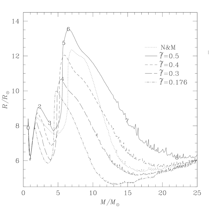
Figure 2.: Mass vs. radius relation for stars on the birthline. The curves labeled $\tilde{f}=0.5,\,0.4,\,0.3,\,0.176$ correspond to accretion rate which are equal to $\tilde{f}$ time the outflow rates given by Churchwell (1998) and Henning et al. (2000), see equation (6). The track N&M is from Norberg & Maeder (2000). Points 1: central ignition of deuterium, 3: start of shell D-burning, 5: end of central contraction; 6: central D-exhaustion, 7: H-ignition, 8: ZAMS

4.2. Sensitivity of the birthline to the accretion rate

Figure 2 shows the relation between the radius and the mass for stars on various theoretical birthlines. The noticeable point is that the higher the accretion rate, the more deuterium is available for burning, the larger the radius and the higher the birthline in the HR diagram.

$$\dot{M}_{\mathrm{accr}}\,\nearrow\,\Longrightarrow\,\textrm{More D-burning}\,\Longrightarrow\ \textrm{Bigger R}\,\Longrightarrow\,\textrm{More luminous birthline}$$

This sensitivity of the birthline to $\dot{M}_{\mathrm{accr}}$ offers an interesting constraint on the accretion rates. This was discussed with some details by Norberg & Maeder (2000). They assume accretion rates of the form

$$\dot{M}_{\mathrm{accr}}=A\,(M/M_{\hbox{$\odot$}})^{\varphi}$$ (4)

and showed that values $A\approx 10^{-5}\,M_{\hbox{$\odot$}}\cdot{\mathrm{yr}}^{-1}$ and $\varphi\approx 1.0-1.5$ are leading to the best fit of the birthline on a large set of observational data for T-Tauri stars and Ae/Be Herbig stars in the HR diagram.

Figure 3.: Time needed by a star to grow from $1$ to $60\,M_{\hbox{$\odot$}}$ at a rate specified by expression (4), as a function of $\varphi$ with $A=10^{-5}\,M_{\hbox{$\odot$}}\cdot{\mathrm{yr}}^{-1}$

The lifetimes $t_{\mathrm{PMS}}$ of the pre–MS phase also depend very much on the accretion rates. Figure 3 shows the duration $t_{\mathrm{PMS}}$ as a function of the exponent $\varphi$ in expression (4). Note that in Tables 1, 2 & 3 of Norberg & Maeder (2000) there is misprint of the decimal point, the ages should be divided by $10$. The rest of numbers in the tables are correct. Figure 3 shows that in order to have pre–MS lifetime of the order of $0.5\cdot 10^{6}\,{\mathrm{yr}}$ or less, it is necessary to have $\varphi\mathrel{\hbox{\hbox to0.0pt{\hbox{\lower 4.0pt\hbox{$\sim$}}\hss}\hbox{$>$}}}1.0$ If this requirement is relaxed to $10^{6}\,{\mathrm{yr}}$, one only needs $\varphi\mathrel{\hbox{\hbox to0.0pt{\hbox{\lower 4.0pt\hbox{$\sim$}}\hss}\hbox{$>$}}}0.6$ These results support the idea that we need accreting rates growing relatively fast with the actual stellar mass.

4.3. Relation with the outflows observed by Churchwell and Henning

Massive outflows have been identified from radio and IR observations by Churchwell (1998) and Henning at al. (2000). The remarkable fact is that there is a relation between the stellar luminosity and the outflow rate $\dot{M}_{\mathrm{out}}$ of the form $\dot{M}_{\mathrm{out}}\propto L^{0.75}$. According to a paper presented by Beuther et al. at this meeting, the relation observed by Churchwell and Henning et al. could rather be an upper envelope of the $\dot{M}_{\mathrm{out}}$ distribution as a function of luminosity. If we adopt a typical mass luminosity relation for stars on the ZAMS in the range $2-85\,M_{\hbox{$\odot$}}$, we get

$$\dot{M}_{\mathrm{out}}\approx 1.5\,10^{-5}\,(M/M_{\hbox{$\odot$}})^{1.5}\,M_{\hbox{$\odot$}}\cdot{\mathrm{yr}}^{-1}.$$ (5)

If we assume that a fraction $f$ of the infalling material is accreted by the star and $(1-f)$ is going into the outflow, we get that a fraction $\tilde{f}=f/(1-f)$ of the outflow mass is effectively accreted, i.e.

$$\dot{M}_{\mathrm{accr}}=\tilde{f}\,\dot{M}_{\mathrm{out}}.$$ (6)

This implies that the accretion rates grow swiftly with the stellar mass, like $M^{1.5}$. This result is quite consistent with what we have found in § 4.2.. Figure 4 shows numerical models by Behrend & Maeder (2001) made with equation (6) and various values of $\tilde{f}$, where $\dot{M}_{\mathrm{out}}$ is taken from data of Churchwell (1998) and Henning et al. (2000). We see that models between those with $\tilde{f}=0.5$ and $0.176$ beautifully reproduce the upper envelope of the observations. A value $\tilde{f}=0.5$ means that one third of the infalling material is effectively accreted, $\tilde{f}=0.176$ means $15\%$. These values are those suggested respectively by the models by Shu et al. (1998) and by the observations by Churchwell (1998).

Figure 4.: Birthlines in the HR diagram for various values of $\tilde{f}$ from Behrend & Maeder (2001). Values $\tilde{f}=0.5$ and $0.176$ correspond to $1/3$ and $15\%$ of the infalling material accreted. A minimum value of $10^{-5}$ M${}_{\hbox{$\odot$}}\cdot{\mathrm{yr}}^{-1}$ is taken for low mass stars. The observations are those collected by Norberg & Maeder (2000); the birthline proposed by these authors is indicated by N& M.

Table 1.: Properties of stars on the birthline with $\tilde{f}=0.176$: age in units of $10^{3}\,{\mathrm{yr}}$, luminosity, mass, effective temperature, radius, relative upper radius of the convective zone, ratio of disc to star luminosities. From models by Behrend & Maeder (2001).

$\begin{array}[]{ccccccc}\hline\cr t&\log(L/L_{\hbox{$\odot$}})&M/M_{\hbox{$\odot$}}&T_{\mathrm{eff}}/{\mathrm{K}}&R/R_{\hbox{$\odot$}}&R_{\mathrm{conv}}^{\mathrm{sup}}/R&L_{\mathrm{disc}}/L\\[2.84526pt] \hline\cr 70.03&1.241&0.7003&4067&8.40&1.000&3.80\\ 80.94&1.099&0.8094&4183&6.74&1.000&6.41\\ 90.32&1.050&0.9032&4276&6.10&1.000&8.27\\ 110.6&1.142&1.106&4402&6.39&1.000&8.41\\ 128.3&1.249&1.283&4460&7.05&1.000&7.97\\ 145.4&1.331&1.454&4515&7.56&1.000&7.67\\ 177.1&1.395&1.771&4615&7.79&1.000&9.04\\ 197.2&1.387&1.972&4731&7.34&1.000&10.7\\ 300.3&1.334&3.003&5060&6.04&1.000&20.6\\ 397.5&1.434&3.975&5354&6.05&1.000&23.8\\ 455.4&2.465&5.014&7579&9.89&0.000&8.04\\ 471.0&2.959&5.985&10.41e3&9.26&0.000&6.49\\ 479.6&3.425&7.022&14.18e3&8.54&0.000&5.24\\ 484.4&3.746&8.002&18.06e3&7.62&0.000&4.86\\ 488.0&3.992&9.038&22.36e3&6.60&0.000&4.87\\ 490.7&4.124&10.01&25.96e3&5.69&0.014&5.49\\ 493.2&4.154&11.02&27.95e3&5.09&0.066&6.54\\ 495.6&4.176&11.99&29.05e3&4.83&0.117&7.72\\ 500.7&4.155&14.01&29.18e3&4.67&0.145&8.77\\ 506.9&4.474&17.03&33.81e3&5.03&0.153&7.82\\ 511.6&4.608&19.98&35.49e3&5.33&0.153&6.62\\ 517.8&4.863&24.98&38.69e3&6.01&0.173&5.41\\ 522.5&5.046&29.88&40.87e3&6.64&0.182&4.72\\ 526.8&5.219&35.20&43.11e3&7.29&0.199&4.05\\ 530.3&5.359&40.46&44.77e3&7.94&0.209&3.61\\ 533.2&5.465&45.24&46.09e3&8.47&0.215&3.31\\ 536.1&5.567&50.56&47.17e3&9.08&0.225&3.03\\ 540.8&5.719&60.56&48.65e3&10.17&0.237&2.60\\ 544.7&5.840&69.98&49.78e3&11.17&0.251&2.38\\ 548.7&5.952&80.65&50.56e3&12.32&0.261&2.15\\ \hline\cr\end{array}$

Table 1 shows some properties of the models by Behrend & Maeder (2001). The disc luminosity is taken as $L_{\mathrm{disc}}={G\,M\,\dot{M}_{\mathrm{inflow}}\over 2\,R}$ with $\dot{M}_{\mathrm{inflow}}=\dot{M}_{\mathrm{out}}+\dot{M}_{\mathrm{accr}}$ (cf. Hartmann 1998). Of course there is a proportionality factor which is uncertain and thus these values for $L_{\mathrm{disc}}$ are only indicative. Table 1 shows that the last stages of massive star accretion go very fast. For example, in Table 1 the time for the evolution from $15$ to $80\,M_{\hbox{$\odot$}}$ is $4.7\ 10^{4}\,{\mathrm{yr}}$. For $\tilde{f}=0.5$, this time would be only $1.5\,10^{4}\,{\mathrm{yr}}$. Of course, for different values of $\varphi$ as in equation (4), we would have different timescales as suggested by Figure 3. As we do not know exactly what is the value of $\varphi$ and $\tilde{f}$, this means that the lifetime for the fast phases of massive star accretion, i.e. from $15\,M_{\odot}$ to $80\,M_{\odot}$ are still rather uncertain, somewhere between a few $10^{4}\,{\mathrm{yr}}$ and a few $10^{5}\,{\mathrm{yr}}$.

5. Models and discussion

5.1. Physics feasibility of the high accretion rate

The accretion rates given by equations (4) and (6) are remarkably well located in the stable zone derived by Wolfire & Cassinelli (1987). For rates lower than a certain limit, the momentum in the radiation pressure is sufficient to prevent the accretion. For rates higher than some limit, the luminosity created by the shock is supra-Eddington. It has been shown by Nakano (1989) that for a non-spherical collapse the stability conditions are much less severe than those given by Wolfire & Cassinelli. In particular, Nakano (1989) suggests that, even for the most massive stars, radiation cannot stop the accretion process and as a consequence he suggests that the maximum stellar mass is determined by fragmentation rather by the accretion process. Certainly, both fragmentation and accretion are essential in shaping the IMF and determining the maximum mass. Indeed, if most of the infalling material is diverted in the outflows, this implies that only a tiny fraction of the initial fragmentats finally contributes to the IMF.

We also point out that the various accretion models do not account for the anisotropy of the radiation field of massive rotating stars, which would favour anisotropic accretion in pre–MS stages and anisotropic mass loss in post–MS phases (cf. Maeder & Desjacques 2001). Indeed, the lower $T_{\mathrm{eff}}$ in the equatorial regions of a rotating massive pre–MS object should very much favour the accretion on these objects. Joined to the above results of Nakano (1989), this supports the idea that accretion at heavy rates of the order of $\dot{M}_{\mathrm{accr}}\approx 10^{-3}\,M_{\hbox{$\odot$}}\cdot{\mathrm{yr}}^{-1}$ is quite possible theoretically.

5.2. Dependence of the accretion rate on the central mass

The location of the birthline, the timescales and the observations of the outflows support accretion rates $\dot{M}_{\mathrm{accr}}\approx 10^{-5}\,(M/M_{\hbox{$\odot$}})^{\varphi}$ with $\varphi\mathrel{\hbox{\hbox to0.0pt{\hbox{\lower 4.0pt\hbox{$\sim$}}\hss}\hbox{$>$}}}1$ as shown above. Globally, we may understand a relation of this kind since for larger masses the central potential is much larger and attracts more matter. The accretion must go like

$$\dot{M}_{\mathrm{accr}}\propto{M\over t_{\mathrm{ff}}}\propto M\,(G\,\bar{\rho})^{1/2}\propto(M/R)^{3/2}$$

where $M$ is the mass of the initial cloud of average density $\bar{\rho}$, $t_{\mathrm{ff}}$ is the free fall time. The radius of the initial subcondensation may vary with their mass in different ways according to different authors. Larson (1981) has suggested for small condensations (Larson’s scaling)

$$\bar{\rho}\propto{1\over R}.$$

If so, $R\propto M^{1/2}$ and thus $\dot{M}_{\mathrm{accr}}\propto M^{3/4}$. In this meeting, Johnstone (2001) has suggested that the density of the subcondensations is constant (Johnstone’s scaling)

$$\bar{\rho}\propto\textrm{const}.$$

In this case, $R\propto M^{1/3}$ and we have

$$\dot{M}_{\mathrm{accr}}\propto M.$$ (7)

Interestingly enough, Johnstone’s scaling implies accretion rate growing almost linearly with the mass as suggested by the observations quoted above. The above arguments are rather schematic and ignore many effects like rotation, accretion disc, outflows, etc. Nevertheless, the general trend they show must be roughly correct. Very detailed numerical models are now in progress in Behrend’s thesis. With finite elements grids, which allow us to follow more closely the interesting parts of the models, the accretion with rotation is modelized, the inflow of the matter through the disc followed as well as the central accretion and outflows. These models predict the accretion rates and should be combined with interior models of the central body.

5.3. Formation of binaries

An apparent difficulty of the accretion scenarios (it is sometimes presented as objection) is the question on how massive binary stars do form. The question is especially important because the fraction of binaries and multiple stars is very high as shown by Zinnecker (this meeting). Here, we would like to suggest some possibilities of preferential binary formation among the OB-stars.

Let us consider a molecular cloud, which is collapsing to give birth to a young star cluster. In the process of cloud fragmentation, some cores may be bound gravitationally, some do not. Each core, bound or not, will accrete matter from its own appropriate Jeans radius. However, the bound or multiple cores will also, in addition to their current accretion, experience a Bondi-Hoyle accretion particularly if their Bondi-Hoyle radius $b$

$$b=2\,{G\,M\over v^{2}}$$ (8)

is greater than the semi-major axis of the supposed double system. In this case, the velocity $v$ appearing in equation (8) is some combination of the orbital velocity in the double system and of the velocity of the double system in the cluster. Thus, double and multiple systems have a higher potential reservoir of matter for accretion and their accretion rates $\dot{M}_{\mathrm{accr}}$ should also be larger than that for single stars.

This means that double and multiple cores, by their larger reservoir and higher $\dot{M}_{\mathrm{accr}}$ will have more chance to move to the top of the mass scale (the IMF) and they will do it faster than the other single objects. This may thus lead to a higher number of double and multiple systems among OB-stars in young clusters. Since mass is accreted on the protobinary system, the semi-major axis will decrease and the orbital periods will also decrease. It is to be examined whether an orbital separation corresponding to the initial tidal radius within the cluster finally leads to periods $P<10\,{\mathrm{d}}$, as so frequently observed in massive O-stars.

In conclusion, we see that many observations and theoretical considerations effectively support the accretion scenario for massive stars. The high frequency of binaries among O–type stars might even be an additional argument in favour of the accretion scenario.

References

Beech, M., & Mitalas, R. 1994, ApJS, 95, 517

Behrend, R., & Maeder, A. 2001, A&A, 373, 190

Bernasconi, P. A., & Maeder, A. 1996, A&A, 307, 829

Bonnell, I. A., Bate, M. R., & Zinnecker, H. 1998, MNRAS, 298, 93

Caselli, P., & Myers, P. C. 1995, ApJ, 446, 665

Cesaroni, R. 2000, Massive Star Birth, ASP Conf. Ser., Eds. P.S. Conti & E.B. Churchwell, in press.

Churchwell, E. 1998 in NATO Science Series, 540, The Origin of Stars and Planetary Systems, ed. C. Lada & N. Kylafis, Kluwer, 515

Elmegreen, B. G. 2000, ApJ, 530, 277

Ezer, D., & Cameron, A. G. W. 1965, AJ, 70, 139

Hartmann, L. 1998 in Accretion processes in Star Formation, Cambridge University Press, 94

Henning, Th., Schreyer, K., Launhardt, R., & Burkert, A. 2000, A&A, 353, 211

Iben, I. Jr. 1963, ApJ, 138, 452

Larson, R. 1981, MNRAS, 194, 809

Maeder, A., & Desjacques, V. 2001, A&A, 372, L9

Morino, J.-I., Yamashita, T., Hasegawa, T., & Nakano, T. 1998, Nature, 393, 340

Nakano, T. 1989, ApJ, 345, 464

Nakano, T., Hasegawa, T., & Norman, C. 1995, ApJ, 450, 183

Nakano, T., Hasegawa, T., Morino, J.-I., & Yamashita, T, 2000, ApJ, 534, 976

Norberg, P., & Maeder, A. 2000, A&A, 359, 1025

Osorio, M., Lizano, S., & D’Alessio, P. 1999, ApJ, 525, 808

Palla, F., & Stahler, S. W. 1993, ApJ, 418, 414

Shu, F., Allen, A., Shang, H., Ostriker, E. C., & Li, Z.-Y. 1998 in NATO Science Series, 540, The Origin of Stars and Planetary Systems, ed. C. Lada & N. Kylafis, Kluwer, 1931

Tatematsu, K., Umemoto, T., Kameya, O., Hirano, N., Hasegawa, T., Hayashi, M., Iwata, T., Kaifu, N., Mikami, H., Murata, Y., Nakano, M., Nakano, T., Ohashi, N., Sunada, K., Takaba, H., & Yamamoto, S. 1993, ApJ, 404, 643

Wolfire, M. G., & Cassinelli, J. P. 1987, ApJ, 319, 850

Wood, D. O. S., & Churchwell, E. 1989, ApJS, 69, 831

Zhang, Q., Hunter, T. R., & Sridharan, T. K. 1998, ApJ, 505, L151