Inhomogeneities in Newtonian Cosmology
and its Backreaction to the Evolution of the Universe

Abstract

We study an effect of inhomogeneity of density distribution of the Universe. We propose a new Lagrangian perturbation theory with a backreaction effect by inhomogeneity. The inhomogeneity affects the expansion rate in a local domain and its own growing rate. We numerically analyze a one-dimensional plane-symmetric model, and calculate the probability distribution functions (PDFs) of several observed variables to discuss those statistical properties. We find that the PDF of pairwise peculiar velocity shows an effective difference from the conventional Lagrangian approach, i.e. even in one-dimensional plane symmetric case, the PDF approaches an exponential form in a small relative-velocity region, which agree with the N-body simulation.

I Introduction

The present Universe shows a variety of structures. How such a structure is formed in the evolution of the Universe. One of the most plausible explanations is that the nonlinear dynamics of a self-gravitating system provides such a scale-free structure during the evolution of the Universe. In order to clarify whether such a dynamics really gives an appropriate observed feature, we have so far three approaches: $N$-body simulation, the Eulerian perturbation approach and the Lagrangian one. Although the final answer for a structure formation would be obtained by the $N$-body simulation, it may be difficult to obtain enough resolution to discuss a fine structure of the Universe such as a scaling property. As for a perturbation approach, however, it is just an approximation and will break down in a nonlinear regime, although the Lagrangian approach would be better if we are interested in density perturbations. This is just because a density fluctuation $\delta$ and a peculiar velocity ${\bf v}$ are perturbed quantities in the Eulerian approach[1], while a displacement of particles from uniform distribution is assumed to be small in the Lagrangian approach[2, 3, 4, 5, 6]. Its first order solution is the so-called Zel’dovich approximation (ZA) [2]. The Lagrangian approach is confirmed to be better than the Eulerian approach by comparison of exact solutions in several cases[7, 8, 9]. Therefore, we will adopt the Lagrangian approximation in this paper and discuss about how to improve it.

In the standard approach of Newtonian cosmology, the global cosmological parameters such as Hubble expansion rate and mean density are given first by a solution of the Einstein equations, i.e. the so-called Friedmann-Robertson-Walker (FRW) universe, which is an isotropic and homogeneous spacetime. According to observation, however, a local structure in the Universe is definitely not homogeneous and isotropic[10]. In the standard approach, the density averaged over the whole space (or a horizon scale) is assumed to be the energy density of the FRW spacetime. However, here the problems of how to average inhomogeneous matter fluid and how to define an averaged isotropic and homogeneous spacetime are arisen. This problem has been discussed in the framework of Newtonian cosmology and general relativity by many authors [11, 12, 13, 14, 15, 16, 17]. The most important point to discuss is how inhomogeneities affect the expansion law of the Universe and whether such a backreaction affects the evolution of the density perturbations. This is our subject to discuss in this paper. Although many authors proposed different methods of averaging procedure in general relativity [11, 12, 13, 14, 15], a serious problem remains. Different gauge choices make the problem more complicated.

Since a relativistic effect may not be so important, in this paper, in order to avoid such a difficulty, we discuss only an averaging procedure in the Newtonian framework. Proposing a averaging procedure, which is defined by spatial average of physical quantities, Buchert and Ehlers lead the averaged Raychaudhuri’s equation[16]. The equation describes how the averaged expansion rate of domain with a finite volume evolves. This equation has an additional term, which we call a ’backreaction term’ of inhomogeneities on averaged expansion. Then, Buchert, Kerscher, and Sicka estimated the backreaction term using the conventional Lagrangian perturbation approach[18]. They first consider density perturbations in Einstein-de Sitter (E-dS) Universe, then calculated the backreaction term and solved the averaged Raychaudhuri’s equation. They showed difference between a cosmological parameter such as Hubble expansion rate in their averaged model and that of the E-dS model. Although they included a backreaction term to estimate the averaged variables in a local domain, they used the perturbed quantities from the E-dS Universe. In other words, they have not take into account a backreaction on the evolution of density perturbations.

Here we improve their approach, i.e. we include a backreaction effect to averaged expansion rate and solve the averaged Raychaudhuri’s equation (the generalized Friedmann’s equation) with evolution equation of perturbations in the averaged domain. In an averaged domain, the averaged density is either higher or lower than that of the E-dS universe. This difference will change the evolution of density perturbations. In fact, if the domain is overdense, growth rate of perturbations behaves as that in the closed universe, While, if it is underdense, it is just like a solution in the open universe.

This paper is organized as follows: In $\S 2$, we shortly derive the generalized Friedmann equation, following Ehlers and Buchert, and estimate a backreaction term. We present our formalism in $\S 3$. We show some relation between two Lagrangian descriptions (the conventional one and ours) and give our initial setting in §. 4. In §5, we analyze a simple example,i.e. a plane-symmetric one-dimensional model, to show the probability distribution of the observed quantities such as Hubble parameter, or density fluctuation, or peculiar velocity. The conclusion and discussion follow in $\S 6$.

II Averaging of inhomogeneity

A The generalized Friedmann equation

In the Newtonian cosmology, the expansion of a domain is influenced by inhomogeneity inside the domain. Such an effect may be evaluated by spatial integration of field variables in the Lagrangian domain, which evolves with matter fluid. Hence in this paper we study fields averaged over a simply-connected spatial Lagrangian domain ${\cal D}$ at time $t$, which evolved out of the initial domain ${\cal D}_{i}$ at time $t_{i}$. The locally averaged scale factor $a_{\cal D}$, depending on the content, shape and location of the domain ${\cal D}$, is defined by the volume of domain $V_{\cal D}(t)=|{\cal D}|$ and its initial volume $V_{{\cal D}_{i}}=|{\cal D}_{i}|$ as

$$a_{\cal D}(t)\equiv\left(\frac{V_{\cal D}(t)}{V_{{\cal D}_{i}}}\right)^{1/3}\,.$$ (1)

We define a spatial averaging for any rank tensor field ${\cal A}=\{A_{ij\cdot}({\bf r},t)\}$ by the volume integral normalized by the volume of the domain as

$$\left<{\cal A}\right>_{\cal D}(t)\equiv\frac{1}{V_{\cal D}(t)}\int_{\cal D}{\rm d}^{3}r\;{\cal A}({\bf r},t)\,.$$ (2)

The average density is then given by

$$\left<\rho\right>_{\cal D}\equiv\frac{M_{\cal D}}{V_{\cal D}(t)}=\frac{M_{\cal D}}{a_{\cal D}^{3}V_{{\cal D}_{i}}}=\frac{1}{a_{\cal D}^{3}}\left<\rho\right>_{{\cal D}_{i}}(t_{i})\propto{a_{\cal D}}^{-3}\,,$$ (3)

where the total mass $M_{\cal D}=\int_{\cal D}{\rm d}^{3}r\;{\cal\rho}({\bf r},t)$ for a domain ${\cal D}$ is conserved. Using this averaging, we can derive the generalized Friedmann equation[16], which we will shortly derive here.

We start from the hydrodynamic equations for a self-gravitating perfect fluid;

$$\frac{\partial\rho}{\partial t}+\nabla_{\bf r}\cdot(\rho{\bf u}) = 0\;,$$ (4)

$$\frac{\partial{\bf u}}{\partial t}+({\bf u}\cdot\nabla_{\bf r}){\bf u} = -\frac{1}{\rho}\nabla_{\bf r}P-\nabla_{\bf r}\Phi\;,$$ (5)

$$\nabla_{\bf r}\times{\bf g} = {\bf 0}\;,$$ (6)

$$\nabla_{\bf r}\cdot{\bf g} = \Lambda-4\pi G\rho\;.$$ (7)

Although it is easy to extend the case with pressure of fluid, we consider just dust matter and ignore a pressure term.

To discuss inhomogeneity, a spatial derivative of field will play a crucial role. In particular, it turns out that the spatial derivative of velocity u, which is divided into three variables as

$$u_{i,j} = \sigma_{ij}+\frac{1}{3}\delta_{ij}\theta+\omega_{ij}\;,$$ (9)

$${\rm with}~{}~{}\omega_{ij}=-\varepsilon_{ijk}\omega^{k}\;,$$

is very important, where

$$\theta = \nabla\cdot{\bf u}~{}~{}~{}~{}~{}~{}~{}~{}~{}~{}~{}~{}~{}~{}~{}~{}~{}~{}~{}~{}~{}~{}~{}~{}~{}~{}~{}({\rm expansion})$$ (10)

$$\sigma_{ij} = \frac{1}{2}(u_{i,j}+u_{j,i})-\frac{1}{3}\delta_{ij}\theta~{}~{}~{}~{}~{}~{}~{}~{}({\rm shear})$$ (11)

$$\omega = \frac{1}{2}\nabla\times{\bf u}~{}~{}~{}~{}~{}~{}~{}~{}~{}~{}~{}~{}~{}~{}~{}~{}~{}~{}~{}~{}~{}~{}~{}~{}({\rm rotation}).$$ (12)

The magnitudes of shear $\sigma$ and of rotation $\omega$ are defined by

$$\sigma=|\underline{\sigma}|\equiv\left(\frac{1}{2}\sigma_{ij}\sigma_{ij}\right)^{1\over 2}\,,\qquad\omega=|\mbox{\boldmath{$\omega$}}|=\left(\frac{1}{2}\omega_{ij}\omega_{ij}\right)^{1\over 2}\;.$$ (13)

Using these variables, we find the basic equations for density, shear and rotation from Eqs. (4), (5) as

$$\dot{\rho} = -\theta\rho\;,$$ (14)

$$\dot{\mbox{\boldmath{$\omega$}}} = -\frac{2}{3}\theta\mbox{\boldmath{$\omega$}}+\underline{\sigma}\cdot\mbox{\boldmath{$\omega$}}\;,$$ (15)

$$\dot{\theta} = \Lambda-4\pi G\rho-\frac{1}{3}\theta^{2}+2(\omega^{2}-\sigma^{2})\;.$$ (16)

The volume of a spatial domain ${\cal D}$ described by its initial domain ${\cal D}_{i}$ through a transformation from the Eulerian coordinates ${\bf r}$ to the Lagrangian one ${\bf q}$ as

$$V_{\cal D}=\int_{\cal D}{\rm d}^{3}r=\int_{{\cal D}_{i}}{\rm d}^{3}qJ_{r}\;,$$ (17)

where $J_{r}$ is the Jacobian of the transformation

$$J_{r}=\det\left(\frac{\partial r_{i}}{\partial q_{j}}\right)\;.$$ (18)

The change rate of the volume of a domain is then given as

$$\frac{1}{V_{\cal D}}\frac{{\rm d}V_{\cal D}}{{\rm d}t} = \frac{1}{V_{\cal D}}\frac{\rm d}{{\rm d}t}\int_{{\cal D}_{i}}{\rm d}^{3}q~{}J_{r}=\frac{1}{V_{\cal D}}\int_{{\cal D}_{i}}{\rm d}^{3}q~{}\dot{J_{r}}$$ (19)

$$= \frac{1}{V_{\cal D}}\int_{{\cal D}_{i}}{\rm d}^{3}q~{}\theta J_{r}=\frac{1}{V_{\cal D}}\int_{{\cal D}}{\rm d}^{3}r~{}\theta=\left<\theta\right>_{\cal D}\;,$$ (20)

where ${\rm d}/{\rm d}t$ denotes the Lagrangian time derivative. Since $\left<\theta\right>_{\cal D}$ is the averaged volume expansion rate of the domain ${\cal D}$, it may be natural to define the effective Hubble expansion rate of the domain ${\cal D}$ by $H_{\cal D}=\left<\theta\right>_{\cal D}/3$. From the definition of the volume $V_{\cal D}$, we find $H_{\cal D}=\dot{a}_{\cal D}/a_{\cal D}$.

The Lagrangian time derivative does not commute with spatial averaging. For an arbitrary tensor field ${\cal A}$, Ehlers and Buchert showed the commutation rule:

$$\frac{{\rm d}\left<{\cal A}\right>_{\cal D}}{\rm dt}-\left<\frac{{\rm d}{\cal A}}{{\rm d}t}\right>_{\cal D}=\left<\theta{\cal A}\right>_{\cal D}-\left<\theta\right>_{\cal D}\left<{\cal A}\right>_{\cal D}\,.$$ (21)

Applying this commutation rule to the basic equations, we find

$$\frac{{\rm d}\left<\rho\right>_{\cal D}}{dt} = -\left<\theta\right>_{\cal D}\left<\rho\right>_{\cal D}\;,$$ (22)

$$\frac{{\rm d}\left<\mbox{\boldmath{$\omega$}}\right>_{\cal D}}{dt} = -\left<\theta\right>_{\cal D}\left<\mbox{\boldmath{$\omega$}}\right>_{\cal D}+\left<\mbox{\boldmath{$\omega$}}\cdot\nabla_{r}{\bf u}\right>_{\cal D}\;,$$ (23)

$$\frac{{\rm d}\left<\theta\right>_{\cal D}}{dt} = \Lambda-4\pi G\left<\rho\right>_{\cal D}+\frac{2}{3}\left<\theta^{2}\right>_{\cal D}-\left<\theta\right>_{\cal D}^{2}+2\left(\left<\omega^{2}\right>_{\cal D}-\left<\sigma^{2}\right>_{\cal D}\right)\;.$$ (24)

Replacing $\left<\theta\right>_{\cal D}$ in Eq. (24) with $3\dot{a}_{\cal D}/a_{\cal D}$ , we find the averaged Raychaudhuri’s equation

$$3\frac{\ddot{a}_{\cal D}}{a_{\cal D}}+4\pi G\left<\rho\right>_{\cal D}-\Lambda=Q_{\cal D}\;,$$ (25)

where

$$Q_{\cal D}\equiv\frac{2}{3}\left(\left<\theta^{2}\right>_{\cal D}-\left<\theta\right>_{\cal D}^{2}\right)+2\left(\left<\omega^{2}\right>_{\cal D}-\left<\sigma^{2}\right>_{\cal D}\right)\;$$ (26)

describes the backreaction due to inhomogeneity of the universe. For $Q_{\cal D}=0$ case, the equation becomes the conventional Friedmann equation with a scale factor $a(t)$ for homogeneous and isotropic universe. This is regarded as the generalized Friedmann equation.

B Evaluation of Backreaction Term $Q_{\cal D}$

In order to evaluate the back reaction term $Q_{\cal D}$, it may be convenient to introduce three principal scalar invariants as follows: For 2-rank tensor field $A=(A_{ij})$  in Cartesian coordinates, those are defined by

$${\bf I}(A_{ij}) = {\rm tr}(A_{ij})\;,$$ (27)

$${\bf II}(A_{ij}) = \frac{1}{2}\left({\rm tr}(A_{ij})^{2}-{\rm tr}\left((A_{ij})^{2}\right)\right)\;,$$ (28)

$${\bf III}(A_{ij}) = {\rm det}(A_{ij})\;.$$ (29)

In particular,for the velocity gradient of matter fluid  $(u_{i,j})$ , we find

$${\bf I}(u_{i,j}) = u_{i,i}=\nabla_{r}\cdot{\bf u}=\theta\;,$$ (30)

$${\bf II}(u_{i,j}) = \frac{1}{2}\left\{(u_{i,i})^{2}-u_{i,j}u_{j.i}\right\}$$ (31)

$$= \frac{1}{2}\nabla_{r}\cdot\left\{{\bf u}(\nabla_{r}\cdot{\bf u})-({\bf u}\cdot\nabla_{r}){\bf u}\right\}$$ (32)

$$= \omega^{2}-\sigma^{2}+\frac{1}{3}\theta^{2}\;,$$ (33)

$${\bf III}(u_{i,j}) = \frac{1}{3}u_{i,j}u_{j,k}u_{k,i}-\frac{1}{2}(u_{i,i})(u_{j,k}u_{k,j})+\frac{1}{6}(u_{i,i})^{3}$$ (34)

$$= \frac{1}{3}\nabla_{r}\cdot\left\{\frac{1}{2}\nabla_{r}\cdot\left({\bf u}(\nabla_{r}\cdot{\bf u})-({\bf u}\cdot\nabla_{r}){\bf u}\right){\bf u}\right.$$ (36)

$$\qquad\left.-\left({\bf u}(\nabla_{r}\cdot{\bf u})-({\bf u}\cdot\nabla_{r}){\bf u}\right)\cdot\nabla_{r}{\bf u}\right\}$$

$$= \frac{1}{9}\theta^{3}+2\theta\left(\sigma^{2}+\frac{1}{3}\omega^{2}\right)-\sigma_{ij}\sigma_{jk}\sigma_{ki}-\sigma_{ij}\omega_{i}\omega_{j}$$ (37)

where we have used the following relations

$$\frac{1}{2}u_{i,j}u_{i,j} = \omega^{2}+\sigma^{2}+\frac{1}{6}\theta^{2}\;,$$ (38)

$$\frac{1}{2}u_{i,j}u_{j,i} = -\omega^{2}+\sigma^{2}+\frac{1}{6}\theta^{2}\;.$$ (39)

Using those invariants, we can describe $Q_{\cal D}$ as

$$Q_{\cal D}=2\left<{\bf II}(u_{i,j})\right>_{\cal D}-\frac{2}{3}\left<{\bf I}(u_{i,j})\right>_{\cal D}^{2}\;.$$ (40)

In the following discussion, we will use the Lagrangian description. Then, it will be convenient to rewrite Eq. (40) by the Lagrangian variables. The Lagrangian domain is just the initial domain ${\cal D}_{i}$. The spatial average of a tensor field $A$ is described by the Lagrangian coordinates as

$$\left<A\right>_{\cal D}=\frac{1}{V_{\cal D}(t)}\int_{{\cal D}}{\rm d}^{3}rA=\frac{\int_{{\cal D}_{i}}{\rm d}^{3}qJ_{r}A}{\int_{{\cal D}_{i}}{\rm d}^{3}qJ_{r}}=\frac{\left<J_{r}A\right>_{{\cal D}_{i}}}{\left<J_{r}\right>_{{\cal D}_{i}}}\;,$$ (41)

where the Lagrangian average $\left<A\right>_{{\cal D}_{i}}$ is defined by

$$\left<A\right>_{{\cal D}_{i}}={1\over V_{{\cal D}_{i}}}\int_{{\cal D}_{i}}{\rm d}^{3}q~{}A$$ (42)

Using this relation, the backreaction term is described by the volume average in the Lagrangian domain ${\cal D}_{i}$ as

$$Q_{\cal D}=\frac{2}{\left<J_{r}\right>_{{\cal D}_{i}}}\left<J_{r}{\bf II}(u_{i,j})\right>_{{\cal D}_{i}}-\frac{2}{3}\left\{\frac{1}{\left<J_{r}\right>_{{\cal D}_{i}}}\left<J_{r}{\bf I}(u_{i,j})\right>_{{\cal D}_{i}}\right\}^{2}\;.$$ (43)

So far, we have not made any approximation. However, when we evaluate those invariants explicitly, we need a further ansatz. Here we adopt a perturbation method. In the conventional perturbation approach, we expand the variables around the background Friedmann universe. In fact, Buchert, Kerscher, and Sicka evaluated the backreaction term $Q_{\cal D}$ by this perturbation method[18], which we will show in the next section. We have also another possibility to divide a perturbed part from a uniform background part as follows: Since we average the variables in some domain and take into account its backreaction effect, we can adopt the averaged variables as unperturbed parts. This way to extract the perturbed parts seems to be more consistent and may provide some difference from the previous approach by Buchert et al. We will discuss the detail next.

III Lagrangian perturbation equations with backreaction

The conventional Lagrangian approximation (for example, ZA [2]) was constructed in a homogeneous and isotropic universe. However, when a nonlinear structure is formed, it is not so clear what is the background universe and how to divide the perturbed part from the unperturbed one. Although the simplest way is the conventional approach, as we discussed in previous section, a local expansion rate of the universe in some finite domain will be affected by its inhomogeneity. Then the growth rate of density fluctuations may also be affected by the inhomogeneity.

We shall derive the consistent equations for the Lagrangian perturbations with the backreaction term $Q_{\cal D}$. First, we introduce the “comoving” Eulerian coordinates ${\bf x}_{b}$ and peculiar velocity ${\bf v}_{b}$ as

$${\bf r} \equiv a_{b}(t){\bf x}_{b}\;,$$ (44)

$${\bf u} \equiv \dot{\bf r}=\dot{a}_{b}(t){\bf x}_{b}+{\bf v}_{b}\;.$$ (45)

In the conventional Lagrangian perturbation approach, we set $a_{b}=a_{H}(t)$ where $a_{H}$ is just a scale factor of the background Hubble flow of the whole universe and satisfies the Friedmann equation. However, because of the above reason, the expansion of a domain ${\cal D}$ may be described by $a_{\cal D}$. Hence, we have not fixed a scale factor $a_{b}$ yet. It will be determined later by adding a further ansatz.

With the relations

$$\nabla_{r} = \frac{1}{a_{b}}\nabla_{{\bf x}_{b}}\;,$$ (46)

$$\left(\frac{\partial f}{\partial t}\right)_{r} = -\frac{\dot{a}_{b}}{a_{b}}({\bf x}_{b}\cdot\nabla_{{\bf x}_{b}})f+\left(\frac{\partial f}{\partial t}\right)_{{\bf x}_{b}}\;,$$ (47)

the basic equations (4)-(7) with $P=0$ are rewritten as

$$\frac{\partial\delta_{b}}{\partial t}+\frac{1}{a_{b}}\nabla_{{\bf x}_{b}}\cdot\{{\bf v}_{b}(1+\delta_{b})\} = 0\;,$$ (48)

$$\left(\frac{\partial{\bf v}_{b}}{\partial t}\right)_{{\bf x}_{b}}+\frac{1}{a_{b}}({\bf v}_{b}\cdot\nabla_{{\bf x}_{b}}){\bf v}_{b}+\frac{{\dot{a}}_{b}}{a_{b}}{\bf v}_{b} = -\frac{1}{a_{b}}\nabla_{{\bf x}_{b}}\left(\Phi+\frac{1}{2}a_{b}\ddot{a}_{b}x_{b}^{2}\right)\;,$$ (49)

$$\triangle_{{\bf x}_{b}}\left(\Phi-\frac{2}{3}\pi G\rho_{b}a_{b}^{2}x_{b}^{2}\right) = 4\pi Ga_{b}^{2}\rho_{b}\delta_{b}-\Lambda a_{b}^{2}\;,$$ (50)

where the density $\rho$ is divided into an unperturbed uniform part $\rho_{b}(t)$, which is defined by the mass conservation $\rho_{b}a_{b}^{3}$= constant, and its fluctuation $\delta$ defined by

$$\delta_{b}\equiv{\rho-\rho_{b}\over\rho_{b}}.$$ (51)

$\Phi$ is the gravitational potential defined by ${\bf g}=-\nabla_{\bf r}\Phi$.

From Eqs. (49) and (50), we obtain the following equation:

$$\left(3\frac{\ddot{a}_{b}}{a_{b}}+4\pi G\rho_{b}\right)+\frac{1}{a_{b}}\nabla_{{\bf x}_{b}}\cdot\left\{\left(\frac{\partial{\bf v}_{b}}{\partial t}\right)_{{\bf x}_{b}}+\frac{1}{a_{b}}({\bf v}_{b}\cdot\nabla_{{\bf x}_{b}}){\bf v}_{b}+\frac{\dot{a}_{b}}{a_{b}}{\bf v}_{b}\right\}+4\pi G\rho_{b}\delta_{b}=0\;.$$ (52)

If we specify $a_{b}$, this equation provides the equation for inhomogeneous part subtracted a background uniform expansion. For example, in the conventional Lagrangian approximation, $a_{b}$ is taken to be a scale factor of the FRW universe $a_{H}$, which satisfies the Friedmann equation

$$3\frac{\ddot{a}_{H}}{a_{H}}+4\pi G\rho_{H}-\Lambda=0\;,$$ (53)

where $\rho_{H}$ is the mean energy density of the universe. On the other hand, if $a_{b}$ is chosen to be $a_{\cal D}$, which evolution is given by the averaged Raychaudhuri’s equation (25), the perturbation equations are modified because of the backreaction effect $Q_{\cal D}$ as

$$\frac{1}{a_{\cal D}}\nabla_{x_{\cal D}}\cdot\left\{\left(\frac{\partial{\bf v}_{\cal D}}{\partial t}\right)_{x_{\cal D}}+\frac{1}{a_{\cal D}}({\bf v}_{\cal D}\cdot\nabla_{x_{\cal D}}){\bf v}_{\cal D}+\frac{{\dot{a}}_{\cal D}}{a_{\cal D}}{\bf v}_{\cal D}\right\}+4\pi G\rho_{\cal D}\delta_{\cal D}=-Q_{\cal D}\;,$$ (54)

where the variables with subscript ${\cal D}$ are defined those with the scale factor $a_{\cal D}$ and $\rho_{\cal D}=\left<\rho\right>_{\cal D}$.

The rotation of (49) yields

$$\nabla_{{\bf x}_{b}}\times\left\{\left(\frac{\partial{\bf v}_{b}}{\partial t}\right)_{{\bf x}_{b}}+\frac{1}{a_{b}}({\bf v}_{b}\cdot\nabla_{{\bf x}_{b}}){\bf v}_{b}+\frac{{\dot{a}}_{b}}{a_{b}}{\bf v}_{b}\right\}=0\;.$$ (55)

Now we will describe those equations in terms of the Lagrangian coordinates. Using the Lagrangian time derivative along the fluid flow

$$\frac{{\rm d}}{{\rm d}t}\equiv\frac{\partial}{\partial t}+\frac{1}{a_{b}}({\bf v}_{b}\cdot\nabla_{{\bf x}_{b}})\,,$$ (56)

Eqs. (54) and (55) are rewritten as

$$\frac{1}{a_{b}}\nabla_{{\bf x}_{b}}\cdot\left(\frac{{\rm d}{\bf v}_{b}}{{\rm d}t}+\frac{\dot{a}_{b}}{a_{b}}{\bf v}_{b}\right)+4\pi G\rho_{b}\delta_{b} = -Q_{b}\;,$$ (57)

$$\nabla_{{\bf x}_{b}}\times\left(\frac{{\rm d}{\bf v}_{b}}{{\rm d}t}+\frac{\dot{a}_{b}}{a_{b}}{\bf v}_{b}\right) = 0\;,$$ (58)

where we have introduced $Q_{b}$, which is zero for the conventional Lagrangian approach without backreaction but is chosen to be $Q_{\cal D}$ when we include the backreaction due to inhomogeneity. Note that there are still some space to estimate this backreaction term depending on a choice of the background scale factor $a_{b}$.

The Lagrangian coordinates ${\bf q}_{b}$, which follows the background flow, is defined by the initial values of the comoving Eulerian coordinates ${\bf x}_{b}$, and the Lagrangian perturbations are described as

$${\bf x}_{b}={\bf q}_{b}+{\bf S}_{b}({\bf q}_{b},t)\;.$$ (59)

where ${\bf S}_{b}$ denotes the displacement from the uniform distribution assuming that the scale factor is given by $a_{b}$. The continuity equation (48) or equivalently the mass conservation yields

$$dM=\rho d^{3}r=\rho a_{b}^{3}d^{3}x_{b}=\rho a_{b}^{3}J_{b}d^{3}q_{b}=\rho_{i}d^{3}q_{b}={\rm constant},$$ (60)

where $J_{b}\equiv{\rm det}(\partial{\bf x}_{bi}/\partial{\bf q}_{bj})={\rm det}(\delta_{ij}+\partial{\bf S}_{bi}/\partial{\bf q}_{bj})$ is the Jacobian of the coordinate transformation ${\bf x}_{b}\rightarrow{\bf q}_{b}$. With $\rho_{b}a_{b}^{3}$= constant, we have

$$\rho\propto\rho_{b}J_{b}^{-1}\,,$$ (61)

or equivalently for density contrast

$$\delta_{b}=J_{b}^{-1}-1\,.$$ (62)

Now all physical quantities are found to be written in terms of ${\bf S}_{b}$ and it remains only to find solutions for ${\bf S}_{b}$. We obtain the following equations for ${\bf S}_{b}$ from equations (57) and (58):

$$\nabla_{{\bf x}_{b}}\cdot\left(\ddot{\bf S}_{b}+2\frac{\dot{a}_{b}}{a_{b}}\dot{\bf S}_{b}\right)=-4\pi G\rho_{b}(J_{b}^{-1}-1)-Q_{b}\,.$$ (63)

$$\nabla_{{\bf x}_{b}}\times\left(\ddot{\bf S}_{b}+2\frac{\dot{a}_{b}}{a_{b}}\dot{\bf S}_{b}\right)=0\,,$$ (64)

In what follows, the subscript $b$ will be dropped except for $a_{b}$ and $\rho_{b}$, but we may put it when we have to distinguish them. In order to write Eqs. (63) and (64) in terms of ${\bf q}$ derivative, we use the relation between $\nabla_{\bf x}$ and $\nabla_{\bf q}\equiv\partial/\partial{\bf q}$, which is given by the definition as

$$\frac{\partial}{\partial q_{i}}=\frac{\partial x_{j}}{\partial q_{i}}\frac{\partial}{\partial x_{j}}=\left(\delta_{ji}+\frac{\partial S_{j}}{\partial q_{i}}\right)\frac{\partial}{\partial x_{j}}=\frac{\partial}{\partial x_{i}}+\frac{\partial S_{j}}{\partial q_{i}}\frac{\partial}{\partial x_{j}}\,.$$ (65)

Using this equation iteratively, we have

$$\frac{\partial}{\partial x_{i}} = \frac{\partial}{\partial q_{i}}-\frac{\partial S_{j}}{\partial q_{i}}\frac{\partial}{\partial x_{j}}$$ (66)

$$= \frac{\partial}{\partial q_{i}}-\frac{\partial S_{j}}{\partial q_{i}}\left(\frac{\partial}{\partial q_{j}}-\frac{\partial S_{k}}{\partial q_{j}}\frac{\partial}{\partial x_{k}}\right)$$ (67)

$$= \frac{\partial}{\partial q_{i}}-\frac{\partial S_{j}}{\partial q_{i}}\frac{\partial}{\partial q_{j}}+\frac{\partial S_{j}}{\partial q_{i}}\frac{\partial S_{k}}{\partial q_{j}}\frac{\partial}{\partial x_{k}}=\cdots\,.$$ (68)

This gives the differential equations in terms of ${\bf q}$ formally. In order to write the basic equations explicitly, however, we need perturbative approach. We then expand the deviation vector ${\bf S}$ as ${\bf S}={\bf S}^{(1)}+{\bf S}^{(2)}+\cdots$. Superscripts $(1)$ and $(2)$ denote first and second order quantities in a perturbative expansion with respect to magnitude of small displacement $\epsilon$ from uniform distribution, respectively. From Eq. (26), the leading terms of the backreaction is second order of $\epsilon$. Then we have to derive the perturbation equations until at least second order. From Eq. (58), we obtain the first and second order equations as follows:

$$\nabla_{q}\times\left(\ddot{\bf S}^{(1)}+2\frac{\dot{a}_{b}}{a_{b}}\dot{\bf S}^{(1)}\right) = 0\;,$$ (69)

$$\left\{\nabla_{q}\times\left(\ddot{\bf S}^{(2)}+2\frac{\dot{a}_{b}}{a_{b}}\dot{\bf S}^{(2)}\right)\right\}_{i} = \varepsilon_{ijk}S^{(1)}_{l|j}\left(\ddot{S}^{(1)}_{k|l}+2\frac{\dot{a}_{b}}{a_{b}}\dot{S}^{(1)}_{k|l}\right)\;.$$ (70)

Next we consider equation (57). The Jacobian $J$ is expanded as

$$J=1+\nabla_{q}\cdot{\bf S}^{(1)}+\nabla_{q}\cdot{\bf S}^{(2)}+\frac{1}{2}\left[(\nabla_{q}\cdot{\bf S}^{(1)})^{2}-S_{i|j}^{(1)}S_{j|i}^{(1)}\right]+\cdots\,.$$ (71)

Thus we obtain the first order equation,

$$\nabla_{q}\cdot\left(\ddot{\bf S}^{(1)}+2\frac{\dot{a}_{b}}{a_{b}}\dot{\bf S}^{(1)}-4\pi G\rho_{b}{\bf S}^{(1)}\right)=0\;,$$ (72)

and the second order one,

$$\nabla_{q}\cdot\left(\ddot{\bf S}^{(2)}+2\frac{\dot{a}_{b}}{a_{b}}\dot{\bf S}^{(2)}-4\pi G\rho_{b}{\bf S}^{(2)}\right)$$ (73)

$$=S^{(1)}_{j|i}\left(\ddot{S}_{i|j}+2\frac{\dot{a}_{b}}{a_{b}}S^{(1)}_{i|j}\right)-2\pi G\rho_{b}\left\{\left(S^{(1)}_{i|i}\right)^{2}+S^{(1)}_{i|j}S^{(1)}_{j|i}\right\}-Q_{b}\;.$$ (74)

In order to solve the above perturbation equations, we decompose ${\bf S}^{(1)}$ and ${\bf S}^{(2)}$ into the longitudinal and the transverse parts in the form

$${\bf S}^{(1)} = \nabla_{q}\psi+\mbox{\boldmath$\psi$}^{T},\;\nabla_{q}\cdot\mbox{\boldmath$\psi$}^{T}=0\;,$$ (75)

$${\bf S}^{(2)} = \nabla_{q}\zeta+\mbox{\boldmath$\zeta$}^{T},\quad\nabla_{q}\cdot\mbox{\boldmath$\zeta$}^{T}=0\;,$$ (76)

where $\psi$ and $\zeta$ are first-order and second-order scalar functions, respectively. As for their physical meanings, the first-order longitudinal and transverse parts are related to linear density and vortical perturbations, respectively. For the second-order level, however, such a simple interpretation of the perturbation modes does not hold any more.

The first-order perturbation equations (72) and (69) become

$$\triangle_{q}\left(\ddot{\psi}+2\frac{\dot{a}_{b}}{a_{b}}\dot{\psi}-4\pi G\rho_{b}\psi\right)=0\;,$$ (77)

$$\nabla_{q}\times\left(\ddot{\mbox{\boldmath$\psi$}}^{T}+2\frac{\dot{a}_{b}}{a_{b}}\dot{\mbox{\boldmath$\psi$}}^{T}\right)=0\;.$$ (78)

The second-order perturbation equations (74) and (70) are also divided into the longitudinal and the transverse parts as

$$\triangle_{q}\left(\ddot{\zeta}+2\frac{\dot{a}_{b}}{a_{b}}\dot{\zeta}-4\pi G\rho_{b}\zeta\right)$$ (79)

$$= 2\pi G\rho_{b}\left\{\psi_{|ij}\psi_{|ij}-(\triangle_{q}\psi)^{2}-\mbox{\boldmath$\psi$}^{T}_{i|j}\mbox{\boldmath$\psi$}^{T}_{j|i}\right\}-Q_{b}\;,$$ (80)

$$\left[\triangle_{q}\times\left(\ddot{\mbox{\boldmath$\zeta$}}^{T}+2\frac{\dot{a}_{b}}{a_{b}}\dot{\mbox{\boldmath$\zeta$}}^{T}\right)\right]_{i}=4\pi G\rho_{b}\varepsilon_{ijk}\mbox{\boldmath$\psi$}^{T}_{l|j}\psi_{|kl}\;.$$ (81)

In what follows, we will fix $a_{b}$ to be $a_{\cal D}$. Note that if we set $a_{b}=a_{H}$, the above equations are equivalent to those by Buchert et al. Since the displacement vector ${\bf S}$ denotes a deviation from homogeneous distribution in the local domain ${\cal D}$, the average density $\rho_{b}=\left<\rho\right>_{\cal D}$, which is written by $\delta_{\cal D}$ in what follows, is not equal to that in the whole universe. The density fluctuation described by ${\bf S}$ should be defined as

$$\delta_{\cal D}=\frac{\rho-\rho_{\cal D}}{\rho_{\cal D}}~{}~{}~{}~{}{\rm with}~{}~{}~{}~{}~{}\left<\delta_{\cal D}\right>_{\cal D}=0\;.$$ (82)

Here we use the subscript ${\cal D}$ to show what is the background mean density.

To solve the above equations, we carry out further procedure. Since the first order equations (77) are the same as those of ZA except for a scale factor, we can easily solve them. The perturbation variables are separated into time and spatial functions as

$$\psi_{\cal D}=b_{\cal D}(t)\varphi_{\cal D}({\bf q})\;.$$ (83)

The evolution equation for $b_{\cal D}$ is

$$\ddot{b}_{\cal D}+2\frac{\dot{a}_{\cal D}}{a_{\cal D}}\dot{b}_{\cal D}-4\pi G\rho_{\cal D}b_{\cal D}=0\;,$$ (84)

while $\varphi_{\cal D}({\bf q})$ is determined from the initial data.

As for the second order equations, we need a little more complicated procedure. In Appendix A, we rewrite the backreaction term $Q_{\cal D}$ in context of the Lagrangian approximation and present its explicit form up to the second order perturbations ($\psi$,$\mbox{\boldmath$\psi$}^{T}$,$\zeta$, and $\mbox{\boldmath$\zeta$}^{T}$). Since the transverse modes ($\mbox{\boldmath$\psi$}^{T}$ and $\mbox{\boldmath$\zeta$}^{T}$) may not be so important, we shall ignore them in what follows. Then the leading order of the backreaction term $Q_{\cal D}$ becomes very simple as

$$Q_{\cal D}=2\left<{\bf II}(\dot{\psi}_{{\cal D}|ij})\right>-\left<{\bf I}(\dot{\psi}_{{\cal D}|ij})\right>^{2}\;,$$ (85)

where $|i=\partial_{{\bf q}_{i}}$ (see Eq. (A26). Using (83), we find

$$Q_{\cal D}=\frac{2}{3}\dot{b}_{\cal D}^{2}\left\{\frac{3}{2}\left<(\triangle_{q_{\cal D}}\varphi_{\cal D})^{2}-\varphi_{{\cal D}|ij}\varphi_{{\cal D}|ji}\right>_{{\cal D}_{i}}-\left<\triangle_{q_{\cal D}}\varphi_{\cal D}\right>_{{\cal D}_{i}}^{2}\right\}\;,$$ (86)

which depends only on time $t$. Eq. (80) for $\zeta_{\cal D}$ is now

$$\triangle_{q}\left(\ddot{\zeta}_{\cal D}+2\frac{\dot{a}_{b}}{a_{b}}\dot{\zeta}_{\cal D}-4\pi G\rho_{b}\zeta_{\cal D}\right)=2\pi G\rho_{\cal D}\left(\psi_{|ij}\psi_{|ij}-(\triangle_{q}\psi)^{2}\right)-Q_{b}\;,$$ (87)

Since the first term of r.h.s. of Eq. (80)

$$2\pi G\rho_{\cal D}b_{\cal D}^{2}\left\{\varphi_{{\cal D}|ij}\varphi_{{\cal D}|ij}-(\triangle_{q}\varphi_{\cal D})^{2}\right\}\;$$ (88)

depends on spatial coordinate ${\bf q}$ as well as $t$, we have to divide a solution into two parts: one is inhomogeneous term and the other is homogeneous one. First, in order to find a homogeneous term, we commute the time and spacial derivatives in Eq. (87), and then integrate it over ${\cal D}_{i}$, finding

$${\frac{{\rm d}^{2}}{{\rm d}t^{2}}\left<\triangle_{q_{\cal D}}\zeta_{\cal D}\right>_{{\cal D}_{i}}+2\frac{\dot{a}_{\cal D}}{a_{\cal D}}\frac{\rm d}{{\rm d}t}\left<\triangle_{q_{\cal D}}\zeta_{\cal D}\right>_{{\cal D}_{i}}-4\pi G\rho_{\cal D}\left<\triangle_{q_{\cal D}}\zeta_{\cal D}\right>_{{\cal D}_{i}}}$$ (89)

$$= 2\pi G\rho_{\cal D}b_{\cal D}^{2}\left<\varphi_{{\cal D}|ij}\varphi_{{\cal D}|ij}-(\triangle_{q_{\cal D}}\varphi_{\cal D})^{2}\right>_{{\cal D}_{i}}-Q_{\cal D}\;,$$ (90)

which is an ordinary differential equation for $\left<\triangle_{q_{\cal D}}\zeta_{\cal D}\right>_{{\cal D}_{i}}$. By Introduction of new variable $\tilde{\zeta}_{\cal D}$ by

$$\triangle_{q_{\cal D}}\tilde{\zeta}_{\cal D}\equiv\triangle_{q_{\cal D}}\zeta_{\cal D}-\left<\triangle_{q_{\cal D}}\zeta_{\cal D}\right>_{{\cal D}_{i}}\;,$$ (91)

we can eliminate the backreaction term $Q_{\cal D}$. The equation for $\tilde{\zeta}_{\cal D}$ is now separable by setting

$$\tilde{\zeta}_{\cal D}=c_{\cal D}(t)\chi_{\cal D}({\bf q})\;,$$ (92)

as

$$\ddot{c}_{\cal D}+2\frac{\dot{a}_{\cal D}}{a_{\cal D}}\dot{c}_{\cal D}-4\pi G\rho_{\cal D}(c_{\cal D}+Ab_{\cal D}^{2})=0\;,$$ (93)

$$\triangle_{q_{\cal D}}\chi_{\cal D}=\frac{\left<{\bf II}(\varphi_{{\cal D}|ij})\right>_{{\cal D}_{i}}-{\bf II}(\varphi_{{\cal D}|ij})}{A}\;,$$ (94)

where $A$ is a separation constant. Finally we obtain a set of basic equations (25),(84), (90), and (93) with the definition (86) for dynamical variables $a_{\cal D}$, $b_{\cal D}$, $\left<\triangle_{q_{\cal D}}\zeta_{\cal D}\right>_{{\cal D}_{i}}$, and $c_{\cal D}$. The spatial inhomogeneities $\varphi_{\cal D}({\bf q})$ and $\chi_{\cal D}({\bf q})$ are determined by initial distributions and Eq. (94).

IV Relation between two Lagrangian descriptions
: Setting up Initial Data

In order to solve our basic equations for Lagrangian perturbations, we have to set up our initial data. Since the initial fluctuation is given by deviation from uniform distribution of the whole universe, which is described by the Eulerian coordinates, we have to construct our initial data from those data by an appropriate transformation. Furthermore, since our equations are valid only in each domain ${\cal D}$, if we wish to analyze some statistical properties of our results, we have to go back to the whole universe. Here we will first discuss such a transformation, and then set up our initial data.

Suppose that we have some inhomogeneous distribution in the Eulerian coordinates ${\bf r}$. We then find $a_{H}$ and $a_{\cal D}$ by integrating a volume over the whole universe and over a domain ${\cal D}$, respectively. Here we set these initial values equal to unity. These scale factors fix ${\bf x}_{H}$ (then ${\bf q}_{H}$ and ${\bf S}_{H}$), and ${\bf x}_{\cal D}$ (then ${\bf q}_{\cal D}$ and ${\bf S}_{\cal D}$). We also find $\rho_{H}$ and $\rho_{\cal D}$ by averaging the density $\rho({\bf r},t)$ over the whole universe and over the domain ${\cal D}$, respectively.

The density perturbation in our basic equations is deviation from a density averaged in a domain ${\cal D}$. Hence a perturbation in the conventional Lagrangian approximation does not satisfy the condition (82). We have to reconstruct initial conditions in our local domain from fluctuations given in the whole universe. In order to set up initial conditions, we may need only the relation between the Eulerian coordinates ${\bf r}$ and our Lagrangian coordinate ${\bf q}_{\cal D}$. However, we also need the relation between two Lagrangian coordinates, ${\bf q}_{\cal D}$ and ${\bf q}_{H}$ from the following reason. In an inhomogeneous universe, we do not know in which domain we are living. Then, when we analyze our results, we need a statistical analysis in the whole universe to know how the observed values are plausible. In particular, one of the most interesting observed values is a peculiar velocity, for which we have to introduce a Hubble flow $a_{H}$ and the comoving Eulerian coordinate ${\bf x}_{H}$. As a result, we need a relation between ${\bf q}_{H}$ and ${\bf q}_{\cal D}$ as well. Note that although both Lagrangian coordinates follow matter fluid, those scales are different. Because we have mass conservation for infinitely small domain (${\bf q}_{\cal D},{\bf q}_{\cal D}+\Delta{\bf q}_{\cal D})$, or equivalently (${\bf q}_{H},{\bf q}_{H}+\Delta{\bf q}_{H})$, i.e.

$$\Delta M=\rho_{H}a_{H}^{3}(\Delta q_{H})^{3}=\rho_{\cal D}a_{\cal D}^{3}(\Delta q_{\cal D})^{3}.$$ (95)

Assuming

$$a_{\cal D}(t_{i})=a_{H}(t_{i})=1\;,$$ (96)

we find

$$\frac{\Delta q_{\cal D}}{\Delta q_{H}}=\left[\frac{\rho_{H}(t_{i})}{\rho_{\cal D}(t_{i})}\right]^{1/3}\;.$$ (97)

Since the density perturbation in the conventional Lagrangian approximation is given by

$$\delta_{H}={\rho-\rho_{H}\over\rho_{H}},$$ (98)

we find $\rho_{\cal D}=\rho_{H}(1+\left<\delta_{H}\right>_{\cal D})$ from the definition of $\rho_{\cal D}$. This gives the relation between $q_{\cal D}$ and $q_{H}$ as

$$\frac{\Delta q_{\cal D}}{\Delta q_{H}}=(1+\left<\delta_{H}(t_{i})\right>_{{\cal D}_{i}})^{-{1\over 3}}\;.$$ (99)

We then find the relation between $\delta_{H}$ and $\delta_{\cal D}$ as follows: From

$$1+\delta_{\cal D}={\rho\over\rho_{\cal D}}={\rho\over\rho_{H}}{\rho_{H}\over\rho_{\cal D}}=(1+\delta_{H}){\rho_{H}(t_{i})\over\rho_{\cal D}(t_{i})}{a_{\cal D}^{3}(t)\over a_{H}^{3}(t)}$$ (100)

with Eq.(99), we find

$$\delta_{\cal D}=\frac{a_{\cal D}^{3}(1+\delta_{H})}{a_{H}^{3}\left[1+\left<\delta_{H}(t_{i})\right>_{{\cal D}_{i}}\right]}-1\;,$$ (101)

We also obtain a peculiar velocity against the Hubble flow as

$${\bf v}_{H}\equiv\dot{{\bf r}}-H{\bf r}=a_{H}\dot{\bf S}_{H}=\left(\dot{a}_{\cal D}-Ha_{\cal D}\right){\bf x}_{\cal D}+a_{\cal D}\dot{\bf S}_{\cal D}\;.$$ (102)

We will use this definition in analysis of a peculiar velocity.

Now we can set up our initial condition. As for the density perturbations, we find from Eq. (101) as

$$\delta_{\cal D}(t_{i})=\frac{(1+\delta_{H}(t_{i}))}{\left[1+\left<\delta_{H}(t_{i})\right>_{{\cal D}_{i}}\right]}-1\;.$$ (103)

From this equation with definitions (62), (71), (75), and (83), we find the initial condition for $\varphi_{\cal D}$ as

$$\triangle_{q}\varphi_{\cal D}=\frac{\left<\delta_{H}(t_{i})\right>_{{\cal D}_{i}}-\delta_{H}(t_{i})}{1+\delta_{H}(t_{i})}\;,$$ (104)

where we set $b_{\cal D}(t_{i})=1$.

As for the scale factor $a_{\cal D}$ of the domain ${\cal D}$, its initial value is set to be unity (Eq.(96)), but its time derivative is non-trivial. In fact, From (20), we find $\dot{a}_{\cal D}$ as

$$\dot{a}_{\cal D}(t_{i})=\dot{a}_{H}(t_{i})\left[1+\frac{1}{3}\left<{\bf I}\left(\psi_{{\cal D},ij}\right)\right>_{{\cal D}_{i}}\right]\;.$$ (105)

V Effect of inhomogeneity

Here, we study a simple model to show new aspect in our approach. We assume a plane-symmetric 1-dimensional model. The Lagrangian perturbation is given by

$$\nabla_{q}\psi={\bf S}({\bf q})=b(t)(s(q_{1}),0,0)\;.$$ (106)

In the conventional Lagrangian approximation, ZA gives an exact solution in a plane-symmetric case. However, it does not take into account a backreaction effect of inhomogeneity on the Hubble expansion. Since our approach includes the backreaction effect, we will analyze this simple one-dimensional model and compare our results with those by ZA. We also look at a difference of the backreaction term estimated by the conventional Lagrangian approach (Buchert et al).

When we consider our backreaction effect, we have a set of equations:

$$\ddot{\psi}_{\cal D}+2\frac{\dot{a}_{\cal D}}{a_{\cal D}}\dot{\psi}_{\cal D}+4\pi G\rho_{\cal D}\psi_{\cal D}=-Q_{\cal D}\,,$$ (107)

$$Q_{\cal D}=\frac{2}{3}\frac{\left(\dot{b}_{\cal D}^{2}\left<{\bf I}_{s}\right>_{{\cal D}_{i}}\right)^{2}}{\left(1+b^{2}\left<{\bf I}_{s}\right>_{{\cal D}_{i}}\right)^{2}}\,.$$ (108)

Since we analyze the present model numerically, we have to introduce the size of ”whole universe”, which is $L$. We the introduce the scale of averaging domain $l$. As for initial conditions, we adopt a power law spectrum with the index $n=1$:

$$P_{i}(k)\propto k\;.$$ (109)

We also introduce a cutoff at small scale, which wave number is $k_{cut}=1024k_{0}$, where $k_{0}=2\pi/L$. We set that the initial time is $a=1$. Then the amplitude of fluctuation is chosen so that the first shell-crossing occurs at $a\simeq 1000$. The number of grids is $N=2^{16}$ and we use a periodic boundary condition. We take an ensemble average over 500 samples, which initial conditions are given by random Gaussian. In our approach, since we do not know where we are living, we study its statistical properties. In particular, we will see the scale dependence of the averaged variables and the probability distribution of the Hubble parameter, deceleration parameter, and pair-wise velocity.

A Hubble parameter

First we analyze the expansion rate of local domain. If we fix the Hubble parameter $H_{0}$ by local observation in a domain ${\cal D}$, the most probable value of $H_{0}$ is given by the averaged expansion rate of the domain, which is $\left<\theta\right>_{\cal D}/3$. Several authors so far discussed such a local measurement of the Hubble parameter [19, 20, 21, 22, 23]. In particular, Shi and Turner [23] estimated a possible value of the Hubble constant measured locally and discussed a deviation from the global value, using linear perturbation theory with the CDM model. They found that for small samples of objects that only extend to 10,000 km $s^{-1}$, the variance can reach 4%, while for large samples of objects to 40,000 km $s^{-1}$, the variance is about 1-2 %.

We solve Eq. (25) for $a_{\cal D}$ with a backreaction due to inhomogeneity. If we are living in an underdense region on average, the expansion rate will be faster than the Hubble one for the whole universe. While, if we stay in an overdense region, the rate will be slower than the global Hubble one. Fig.1 shows the PDF of a local Hubble parameter in our calculation. If our domain is small, the deviation from $H_{0}$ gets large. For example, the dispersion of the Hubble parameter is about 1.2 % for the $l=128$-grid domain, while 0.66 % for the$l=256$-grid domain. The dispersion of our model is consistent with the result by Shi and Turner.

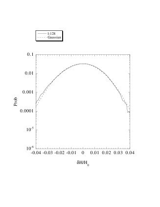
FIG. 1.: The PDF of the Hubble parameter at $a=900$ for $l=128$-grid domain. The dispersion is 1.2 %.

B Density fluctuation

Next we show the PDF of density fluctuations. In the Eulerian linear approximation, if initial data is given by random Gaussian distribution, the PDF of density fluctuations will remain its Gaussian form during evolution. On the other hand, in the Lagrangian approximation, there appears a nonlinear effect. In fact, Kofman et al shows that the PDF approaches to a log-normal function rather than a Gaussian function in the cases of the Lagrangian approximation and N-body simulation[24]. Padmanabhan and Subramanian also discussed the PDF with the ZA and found a non-Gaussian distribution[25].

Here we analyze the PDF of density fluctuations using our approximation. The results are shown in Fig.2. From comparison with the result of ZA, the void region (i.e. an underdense region; $\delta<0$) is found in higher probability in our approximation. Especially, if the size of a domain is smaller, the difference gets larger. On the other hand, the probability to find an overdense region ($\delta>0$) decreases in our approximation.

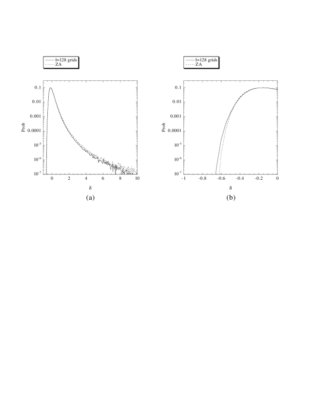
FIG. 2.: The PDF of density fluctuation at $a=900$ for $l=128$-grid domain and that with the ZA. The probability to find an overdense region for $l=128$-grid domain is less than that with the ZA((a)). On the other hand, the probability for an underdense region increases for $l=128$-grid domain((b)).

The reason is very simple: During evolution, an overdense region shrinks and a nonlinear structure is formed as the Zel’dovich’s pancake. On the other hand, an underdense region expands. Therefore, although the initial volumes of overdense underdense regions are the same, the volume of the latter gets larger than that of the former in a nonlinear stage. In addition to this Lagrangian nonlinear effect, we take into account a backreaction effect. This effect enhances expansion of an underdense region and contraction of an overdense region. As a result, the above difference between ZA and our approximation appears.

C Peculiar velocity distribution

In the conventional Lagrangian approximation, if an initial condition is given by a random Gaussian distribution, the PDF of a peculiar velocity also remains its Gaussian form[24]. Because a peculiar velocity ${\bf v}_{H}$ in the conventional Lagrangian approximation (or the ZA) is given by

$${\bf v}_{H}=a_{H}\dot{\bf S}_{H}\;,$$ (110)

the spectrum of a peculiar velocity is proportional to that of a density fluctuation as $P_{v}(k)\propto(\dot{b}/B)^{2}P_{\delta}(k)$. However, in our case, a peculiar velocity is given by (102) and the growing factor $b_{\cal D}$ is different in each domain, the PDF could deviate from a Gaussian distribution. However, from our numerical analysis (see Fig. 3), the PDF of a peculiar velocity seems to still be a Gaussian. This may be because we need only a linear term of the Lagrangian perturbations in the present analysis.

FIG. 3.: The PDF of peculiar velocity at $a=900$ for $l=128$ grid domain. The PDF obeys Gaussian form.

D Pairwise peculiar velocity distribution

The PDF of a radial pairwise peculiar velocity is known to show an exponential form from analysis of N-body simulation and the ZA [26, 27]. For this variable, even if initial data is given by a random Gaussian distribution, the PDF approaches an exponential form as the universe evolves[27]. The origin of this result could be understood by nonlinearity of gravity. In the case of one-dimensional plane-symmetric system in the conventional Lagrangian approximation (in fact, the ZA is exact), we do not find any non-Gaussian structure. However, even in the ZA, the PDF shows non-Gaussian behavior in the case of three-dimensional case[27]. If we take into account our backreaction effect, does non-Gaussian behavior emerge even in one-dimensional case ?

The pairwise peculiar velocity is defined as follows:

$${\bf v}_{AB}(t) \equiv {\bf v}_{B}(t)-{\bf v}_{A}(t)$$ (111)

$$\equiv {\bf v}_{\parallel}(t)+{\bf v}_{\perp}\;,$$ (112)

where ${\bf v}_{\parallel}$ and ${\bf v}_{\perp}$ represent components parallel and perpendicular to ${\bf x}_{AB}\equiv{\bf x}_{B}-{\bf x}_{A}$, respectively. In a plane-symmetric case, ${\bf v}_{\parallel}$ only appears. Hereafter we write this by $\tilde{v}$. If matter distribution is clustering, $\tilde{v}$ is expected to be negative.

Giving initial data by random Gaussian, the PDF of a pairwise peculiar velocity is Gaussian at initial time. During evolution, the PDF will deviate from Gaussian. In fact, from Fig.4, which shows the PDF of a peculiar velocity in nonlinear regime, we find that it is not Gaussian and approaches an exponential form in a small velocity region. As a reference, we show that the PDF for the ZA, which shows a Gaussian form. The reason may be understood as follows: In a plane-symmetric model, gravitational potential is proportional to a distance between two sheets ($\psi\sim|r|$). Then, even if two sheets approaches very closely, a gravitational force does not become strong but keep constant. When we take into account a backreaction effect, however, a gravitational force will be strong in a clustering region, because the expansion rate of a local domain is slow down. The strengthening of a gravitational force in a cluster region may make a deviation of the PDF of pairwise peculiar velocity from its Gaussian form. Note that in the 3D system, which shows non-Gaussian PDF, a gravitational force increases when two particles approach.

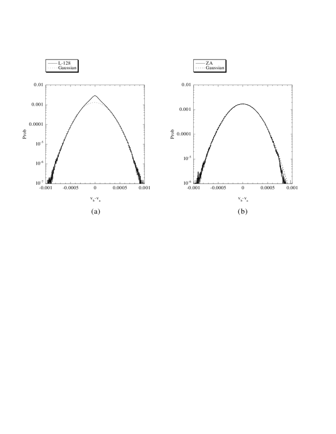
FIG. 4.: The PDF of pairwise peculiar velocity at $a=900$ for $l=128$-grid domain (a) and E-dS model (b). The PDF in (a) does not obey Gaussian form, and approaches to log-normal form at small velocity region. On the other hand, the PDF in (b) obeys Gaussian form.

E Deceleration parameter $q$

Another interesting observable variable is a deceleration parameter. The recent observation of type Ia supernova may suggest an acceleration of the Universe[29]. Although this result may naively suggest an existence of dark energy such as a cosmological constant $\Lambda$, we could find some effective model without dark energy which explain the observation. Then we shall estimate a deceleration parameter averaged in a local domain here.

We define local deceleration parameter $q_{\cal D}$ as

$$q_{\cal D}\equiv-\frac{a_{\cal D}\ddot{a}_{\cal D}}{\dot{a}_{\cal D}^{2}}\;,$$ (113)

which can be evaluated by Eq. (25) and $H_{\cal D}$. Buchert et al[18] showed the evolution of deceleration parameter for the ZA. They picked up overdense and underdense regions of three-$\sigma$ fluctuations and found that $q_{\cal D}$ for an underdense region could be a present day value, which is smaller by more than 200% than that of the background E-dS Universe, although such a region is still decelerating.

Although our approach includes a backreaction consistently, our analysis shows that a deviation of $q_{\cal D}$ does not get so large. The difference of $q_{\cal D}$ from the ZA is very little even just before the shell crossing. We show the time evolution of $q_{\cal D}$ for a plane-symmetric 1-dimensional model in Fig. 5. Even if a domain is extremely underdense, the domain is decelerating. This may be because our approach is still perturbative. We will discuss it further in the next section.

FIG. 5.: The evolution of a deceleration parameter $q_{\cal D}$ for $l=64$-grid domain. The overdense domain shows increase of $q_{\cal D}$ (a solid line for maximum value), while the underdense domain shows decrease of $q_{\cal D}$ (a dashed line for minimum value).

VI Conclusion and Remarks

We propose new Lagrangian perturbation theory with a backreaction effect by inhomogeneity of density perturbations and present a set of basic equations. The inhomogeneity affects the expansion rate in a local domain and its own growing rate. In a one-dimensional plane-symmetric model, we have numerically analyzed our approach, and calculated the growing rate density perturbations and the PDF of several observed variables. We set our initial conditions as random Gaussian distribution. From our analysis, we show that the expansion rate of an overdense region is faster than that of the whole universe as expected. We also show that the local Hubble parameter may deviate from the global one by about 1.2 % for a $l=128$-grid domain. It may be too small to distinguish its effect in the present observations[28], but it could become important in fully non-linear stage, which we cannot describe in the present approach.

The PDF of density is slightly different from that of the ZA. In our model, an underdense region expands faster than that in the E-dS model and then its volume gets larger. Hence, a probability for a negative $\delta$ region increases as seen in the PDF. As for a peculiar velocity, even if we take into account a backreaction, its PDF is still Gaussian.

The PDF of pairwise peculiar velocity, however, shows an effective difference from the conventional Lagrangian approach. In one-dimensional plane symmetric case, the PDF in the conventional Lagrangian approximation (the ZA) is Gaussian, but ours is not but approaches an exponential form in a small relative-velocity region, which agree with the N-body simulation and the 3D Lagrangian approximation[26, 27].

Finally, we mention about recent observation about cosmological parameters. According to the observation of type Ia supernova, the expansion of the Universe seems to accelerate[29]. Combining observation of the cosmic microwave background radiation (CMBR), the result suggests existence of dark energy such as a cosmological constant $\Lambda$[30]. However, this produces another difficulty, that is the so-called cosmological constant problem. To avoid such a difficulty, if we could explain the observation without cosmological constant, it would be more natural. Recently, Tomita discussed such possibility assuming we are in a large local void[31, 32, 33]. Globally the Universe is flat (EdS universe), but we are sitting near the center of a local void, which existence is observationally confirmed. Then he calculated the luminosity distance, finding that the observation can be explain by such a model. We then wonder whether we could have the similar explanation if we are living in an effective void, which is a domain with an averaged energy density below the critical value. Since we have to treat a strongly nonlinear structure to explain the observation, this is beyond our present approach. However there is some indication. If we analyze the time dependence of the backreaction term $Q_{\cal D}$, which evolves as $a^{-1}$ in a linear perturbation level. This time dependence is the same as a perfect fluid with the equation of state $P=-{2\over 3}\rho$, which could be dark energy. If we could explain the above observation without introduction of any strange matter but just by inhomogeneity of density distribution in the Universe, we will have a natural understanding of the Universe. This is under investigation.

In addition, there are two further approaches which are related to the present work. Takada and Futamase[34] proposed that they divided Lagrangian perturbation to large-scale and small-scale perturbations, then discussed interaction between those scales. Taruya and Soda[35] discussed dynamics of averaged variables in the case of a spherical infall model taking into account a backreaction effect. Since those are interesting approaches, it may be useful to use their approaches to discuss the present subject and compare those results with ours in future.

A backreaction in Lagrangian approximation

Using the Lagrangian approximation, we estimate a backreaction term $Q_{\cal D}$. Using the Lagrangian perturbation ${\bf S}$, we shall rewrite the backreaction term. For convenience, first we define the functional determinant of three functions $A({\bf q}),B({\bf q}),C({\bf q})$:

$${\cal I}(A,B,C)\equiv\frac{\partial(A,B,C)}{\partial(q_{1},q_{2},q_{3})}=\varepsilon_{ijk}A_{|i}B_{|j}C_{|k}\;.$$ (A1)

The invariants of the velocity gradient $u_{i,j}$ are given in terms of functional determinants as

$$u_{i,j} = \frac{1}{2J_{r}}\varepsilon_{jkl}{\cal J}(\dot{r}_{i},r_{k},r_{l})\;,$$ (A2)

$${\bf I}(u_{i,j}) = \frac{1}{2J_{r}}\varepsilon_{ijk}{\cal J}(\dot{r}_{i},r_{j},r_{k})\;,$$ (A3)

$${\bf II}(u_{i,j}) = \frac{1}{2J_{r}}\varepsilon_{ijk}{\cal J}(\dot{r}_{i},\dot{r}_{j},r_{k})\;.$$ (A4)

Introducing The r.h.s. of the Lagrangian coordinates $q_{i}$ and perturbations $S_{i}$ by $r_{i}=a(t)(q_{i}+S_{i})$, the r.h.s. of these equations are rewritten as

$${\cal J}(\dot{r}_{i},r_{j},r_{k}) = a^{2}\dot{a}\left[{\cal J}(q_{i},q_{j},q_{k})+3{\cal J}(S_{i},q_{j},q_{k})+3{\cal J}(S_{i},S_{j},S_{k})+{\cal J}(S_{i},S_{j},S_{k})\right]$$ (A6)

$$+a^{3}\left[{\cal J}(\dot{S}_{i},q_{j},q_{k})+2{\cal J}(\dot{S}_{i},S_{j},q_{k})+{\cal J}(\dot{S}_{i},S_{j},S_{k})\right]\;,$$

$${\cal J}(\dot{r}_{i},\dot{r}_{j},r_{k}) = a\dot{a}^{2}\left[{\cal J}(q_{i},q_{j},q_{k})+3{\cal J}(S_{i},q_{j},q_{k})+3{\cal J}(S_{i},S_{j},q_{k})+{\cal J}(S_{i},S_{j},S_{k})\right]$$ (A9)

$$+2a^{2}\dot{a}\left[{\cal J}(\dot{S}_{i},q_{j},q_{k})+2{\cal J}(\dot{S}_{i},S_{j},q_{k})+{\cal J}(\dot{S}_{i},S_{j},S_{k})\right]$$

$$+a^{3}\left[{\cal J}(\dot{S}_{i},\dot{S}_{j},q_{k})+{\cal J}(\dot{S}_{i},\dot{S}_{j},S_{k})\right]\;.$$

Introducing a simplified description follows:

$${\bf I}_{s}\equiv{\bf I}(S_{i|j})\;,\;{\bf II}_{s}\equiv{\bf II}(S_{i|j})\;,\;{\bf III}_{s}\equiv{\bf III}(S_{i|j})\;,$$ (A10)

$${\bf I}_{\dot{s}}\equiv{\bf I}(\dot{S}_{i|j})\;,\;{\bf II}_{\dot{s}}\equiv{\bf II}(\dot{S}_{i|j})\,,\;{\bf III}_{\dot{s}}\equiv{\bf III}(\dot{S}_{i|j})\;,$$ (A11)

we find that most terms in (A2)-(A4) with (A6), (A9) are given by the following quantities;

$$\varepsilon_{ijk}{\cal J}(q_{i},q_{j},q_{k})=6\;,~{}~{}~{}~{} ~{}~{}~{}~{}\varepsilon_{ijk}{\cal J}(S_{i},q_{j},q_{k})=2{\bf I}_{s}\;,$$ (A12)

$$\varepsilon_{ijk}{\cal J}(S_{i},S_{j},q_{k})=2{\bf II}_{s}\;,~{}~{}~{}~{} ~{}~{}~{}~{}\varepsilon_{ijk}{\cal J}(S_{i},S_{j},S_{k})=6{\bf III}_{s}\;,$$ (A13)

$$\varepsilon_{ijk}{\cal J}(\dot{S}_{i},q_{j},q_{k})=2{\bf I}_{\dot{s}}\;,~{}~{}~{}~{} ~{}~{}~{}~{}\varepsilon_{ijk}{\cal J}(\dot{S}_{i},\dot{S}_{j},q_{k})=2{\bf II}_{\dot{s}}\;.$$ (A14)

${\cal J}(\dot{S}_{i},S_{j},q_{k})$ and ${\cal J}(\dot{S}_{i},S_{j},S_{k})$ are written as

$$\varepsilon_{ijk}{\cal J}(\dot{S}_{i},S_{j},q_{k}) = \frac{\partial}{\partial t}{\bf II}_{s}\;,$$ (A15)

$$\varepsilon_{ijk}{\cal J}(\dot{S}_{i},S_{j},S_{k}) = 2\frac{\partial}{\partial t}{\bf III}_{s}\;,$$ (A16)

but the last term ${\cal J}(\dot{S}_{i},\dot{S}_{j},S_{k})$ cannot be written by any of ${\bf I}_{s}$, ${\bf II}_{s}$, ${\bf III}_{s}$ and those time derivatives.

We then finally obtain

$$J_{r}{\bf I}(u_{i,j}) = \frac{1}{2}\left\{6a^{2}\dot{a}\left(1+{\bf I}_{s}+{\bf II}_{s}+{\bf III}_{s}\right)+2a^{3}\left({\bf I}_{\dot{s}}+2\frac{\partial}{\partial t}{\bf II}_{s}+\frac{\partial}{\partial t}{\bf III}_{s}\right)\right\}\;,$$ (A17)

$$J_{r}{\bf II}(u_{i,j}) = \frac{1}{2}\left[6a\dot{a}^{2}\left(1+{\bf I}_{s}+{\bf II}_{s}+6{\bf III}_{s}\right)\right.$$ (A20)

$$\quad+4a^{2}\dot{a}\left(1+{\bf I}_{\dot{s}}+\frac{\partial}{\partial t}{\bf II}_{s}+\frac{\partial}{\partial t}{\bf III}_{s}\right)$$

$$\quad\left.+2a^{3}\left\{{\bf II}_{\dot{s}}+\varepsilon_{ijk}{\cal J}(\dot{S}_{i},\dot{S}_{j},S_{k})\right\}\right]\;.$$

Using these invariants, we find a backreaction term in terms of the Lagrangian perturbations as

$$Q_{\cal D} = \frac{2}{3}\frac{1}{(1+\left<{\bf I}_{s}\right>_{{\cal D}_{i}}+\left<{\bf II}_{s}\right>_{{\cal D}_{i}}+\left<{\bf III}_{s}\right>_{{\cal D}_{i}})^{2}}$$ (A25)

$$\times\left[3(1+\left<{\bf I}_{s}\right>_{{\cal D}_{i}}+\left<{\bf II}_{s}\right>_{{\cal D}_{i}}+\left<{\bf III}_{s}\right>_{{\cal D}_{i}})\right.$$

$$\left(\left<{\bf II}_{\dot{s}}\right>_{{\cal D}_{i}}+\left<\varepsilon_{ijk}{\cal J}(\dot{S}_{i},\dot{S}_{j},S_{k})\right>_{{\cal D}_{i}})\right.$$

$$\left.-\left(\left<{\bf I}_{\dot{s}}\right>_{{\cal D}_{i}}+2\left<\frac{\partial}{\partial t}{\bf II}_{s}\right>_{{\cal D}_{i}}+\left<\frac{\partial}{\partial t}{\bf III}_{s}\right>_{{\cal D}_{i}}\right)^{2}\right]\;.$$

If we take into account the perturbations up to the second order, we find

$$Q_{\cal D} = 2\left<{\bf II}_{\dot{s}}\right>_{{\cal D}_{i}}-\frac{2}{3}\left<{\bf I}_{\nabla_{q}\dot{\varphi}}\right>_{{\cal D}_{i}}^{2},$$ (A26)

where we use the variables in Eqs. (75) and (76). Note that the second order perturbation $\zeta$ do not appear in Eq. (A26).

Buchert et al estimated the backreaction term $Q_{\cal D}$ assuming ZA, i.e. $a_{b}=a_{H}$ and the Lagrangian perturbation ${\bf S}$ is separable as

$${\bf x}={\bf q}+b(t)\nabla_{q}\varphi({\bf q})\;,$$ (A27)

and found the similar form to (A25).[18]