Gravitational Microlensing Events Due to Stellar Mass Black Holes

Abstract

We present an analysis of the longest timescale microlensing events discovered by the MACHO Collaboration during a seven year survey of the Galactic bulge. We find six events that exhibit very strong microlensing parallax signals due, in part, to accurate photometric data from the GMAN and MPS collaborations. The microlensing parallax fit parameters are used in a likelihood analysis, which is able to estimate the distance and masses of the lens objects based upon a standard model of the Galactic velocity distribution. This analysis indicates that the most likely masses of five of the six lenses are $>1\,\rm{M_{\odot}}$, which suggests that a substantial fraction of the Galactic lenses may be massive stellar remnants. This could explain the observed excess of long timescale microlensing events. The lenses for events MACHO-96-BLG-5 and MACHO-98-BLG-6 are the most massive, with mass estimates of $M/\rm{M_{\odot}}=6{+10\atop-3}$ and $M/\rm{M_{\odot}}=6{+7\atop-3}$, respectively. The observed upper limits on the absolute brightness of main sequence stars for these lenses are $<1\,\rm{L_{\odot}}$, so both lenses are black hole candidates. The black hole interpretation is also favored by a likelihood analysis with a Bayesian prior using a conventional model for the lens mass function. We consider the possibility that the source stars for some of these six events may lie in the foreground Galactic disk or in the Sagittarius (SGR) Dwarf Galaxy behind the bulge, but we find that bulge sources are likely to dominate our microlensing parallax event sample. Future HST observations of these events can either confirm the black hole lens hypothesis or detect the lens stars and provide a direct measurement of their masses. Future observations of similar events by SIM or the Keck or VLTI interferometers (Delplancke, Górski & Richichi, 2001) will allow direct measurements of the lens masses for stellar remnant lenses as well.

1 Introduction

The abundance of old stellar remnants in our Galaxy is largely unknown because they emit little radiation unless they happen to be accreting material from a companion star, or for neutron stars, if they happen to emit pulsar radiation in our direction. Gravitational microlensing surveys (Liebes, 1964; Paczyński, 1986; Alcock et al., 1993; Aubourg et al., 1993; Udalski et al., 1993; Bond et al., 2001) have the potential to detect completely dark stellar remnants, but for most microlensing events, the mass can only be estimated very crudely based upon the observed Einstein ring diameter crossing time, $\widehat{t}$. For an individual microlensing event, the mass can only be estimated so crudely that a $7\rm{M_{\odot}}$ black hole cannot be distinguished from a $0.5\rm{M_{\odot}}$ star. However, for some microlensing events, it is possible to measure other parameters besides $\widehat{t}$ that allow tighter constraints on the lens mass (Refsdal, 1966; Gould, 1992; Nemiroff & Wickramasinghe, 1994; Alcock et al., 1995; Bennett et al., 1996; Han & Gould, 1997; Alcock et al., 1997c; Afonso et al., 2000; Alcock et al., 2001a). For long timescale microlensing events, which are often due to massive lenses, it is frequently possible to measure the microlensing parallax effect (Refsdal, 1966; Gould, 1992; Alcock et al., 1995) which is an observable deviation in the microlensing light curve due to the orbital motion of the Earth. In this paper, we present an analysis of the microlensing events discovered by the MACHO Project which give a very strong microlensing parallax signal, and we show that some of these events are best explained as microlensing by black holes.

This paper is organized as follows: in Sections 2 and 3, we discuss the microlensing event data set and the long timescale sub-sample. The microlensing parallax fits are presented in Section 4, and in Section 5 we present our main analysis to determine the distances and masses of the lenses. This includes a discussion of the projected lens velocity distributions, the source star color magnitude diagrams, and a likelihood analysis of the distances and masses of the microlenses. In Section 6, we discuss possible follow-up observations with high resolution telescopes and interferometers that can directly determine the microlensing parallax event lens masses, and we conclude in Section 7.

2 The Data Set

The MACHO Project (Alcock et al., 1993) has monitored $\sim 10-20$ million stars in the Galactic bulge for 6-7 months per year during each of the 1993-1999 Galactic bulge seasons. During the last half of 1994, real-time microlensing discovery with the MACHO Alert system became possible (Alcock et al., 1996). (The OGLE collaboration developed this capability the same year (Udalski et al., 1994b).) This development allowed much more accurate photometry of the microlensing events, which were discovered in progress, from the CTIO 0.9m telescope where the MACHO/GMAN Project was allocated about 1 hour every night (Becker, 2000). In 1997, the Microlensing Planet Search (MPS) Project (Rhie et al., 1999) began microlensing follow-up observations from the Mt. Stromlo 1.9m telescope.

The data set used for this analysis consists of the MACHO survey data from the Mt. Stromlo 1.3m “Great Melbourne” telescope for all seven years, CTIO 0.9m data of selected alert events from 1995-1999, and Mt. Stromlo 1.9m data of alert events from the MPS 1997-1999 data sets. The initial selection of events consists of 42 events from 1993 (Alcock et al., 1997b), 252 events discovered by the MACHO Alert system from 1995-1999 (available from http://darkstar.astro.washington.edu/), and an additional 27 events discovered during the testing of the alert system, for a grand total of 321 events. There are $\sim 200$ additional Galactic bulge events that have been discovered via other analyses that we have not considered here. This paper will focus on the six events from this list which give a strong microlensing parallax signal. The coordinates of these events are given in Table 1. A microlensing parallax study of a larger number of MACHO Alert events is presented in Becker (2000).

The MACHO and MPS data were reduced with slightly different versions of the SoDOPHOT photometry code (Bennett et al., 1993; Alcock et al., 1999). SoDOPHOT is quite similar to the DOPHOT photometry code (Schechter, Mateo, & Saha, 1993) that it was derived from, but SoDOPHOT photometry generally exhibits smaller photometric scatter than DOPHOT photometry. This is due, in part, to SoDOPHOT’s error flags which allow the removal of suspect data points (Alcock et al., 1999), but the scatter in DOPHOT photometry is often increased by the user’s choice of PSF fitting parameters. Contrary to expectations, allowing the PSF fit box size to scale with the seeing generally causes increased photometric scatter (Bennett et al., 1993). The photometric errors reported by SoDOPHOT are modified by adding of 1.4% and 1.0% in quadrature to the MACHO and MPS data, respectively, to account for normalization and flat fielding errors. The CTIO data were reduced with the ALLFRAME package (Stetson, 1994), with the error estimates multiplied by a factor of 1.5 to account for systematic errors.

Table 2 gives the number of observations in each pass band for each event, and the data used for this paper are presented in Table 3. The complete set of macho survey data is available at http://wwwmacho.mcmaster.ca/ and http://wwwmacho.anu.edu.au. Only the MACHO survey data has been calibrated and transformed to standard pass bands (Alcock et al., 1999). The other data is given in instrumental magnitudes which have only been calibrated relative to other measurements with the same telescope and passband. The transformation between raw MACHO magnitudes given in Table 3 ($B_{\rm MACHO}$ and $R_{\rm MACHO}$) and the Kron-Cousins $V$ and $R$ system is given by:

$$V = 2.699+a\,B_{\rm MACHO}+b\,R_{\rm MACHO}$$

$$R = 2.412+c\,B_{\rm MACHO}+d\,R_{\rm MACHO}\ ,$$ (1)

where the coefficients, $a$, $b$, $c$, and $d$ are slightly different for each event as shown in Table 4.

3 Long Timescale Events

The timescale of a gravitational microlensing event is described by the Einstein diameter crossing time, $\widehat{t}$, which depends on the lens mass ($M$), distance ($D_{\ell}$), and transverse velocity ($v_{\rm\perp}$). It is given by

$$\widehat{t}={2R_{E}\over v_{\rm\perp}}={4\over v_{\rm\perp}c}\sqrt{GMD_{\ell}(D_{s}-D_{\ell})\over D_{s}}\ ,$$ (2)

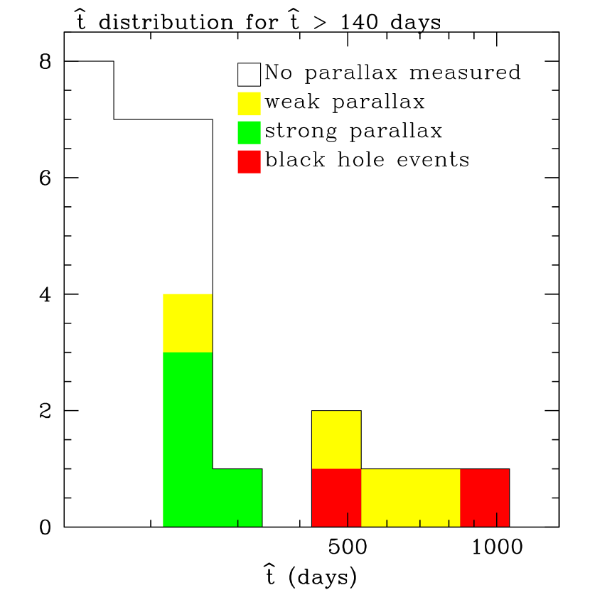
Figure 1: The distribution of event timescales, $\widehat{t}$, for the 28 events with $\widehat{t}>140\,$ days. The colored bars indicate the events with formally significant detections of microlensing parallax, but parallax signal for the events indicated in yellow is weak enough that the detection is not considered to be definitive.

where $D_{s}$ refers to the distance to the source (typically $8\,$kpc for a bulge source), and $R_{E}$ is the radius of the Einstein Ring. Eq. (2) indicates that long $\widehat{t}$ events can be caused by large $M$, small $v_{\rm\perp}$ or both. Fig. 1 shows the long timescale tail of the $\widehat{t}$ distribution for our sample of 321 Galactic bulge microlensing events. In their analysis of the timescale distribution of the 1993 MACHO and OGLE bulge data sets, Han & Gould (1996) noted a surprisingly large fraction of the events with $\widehat{t}\geq 140\,$days: 4/51 or 8%. Such a large fraction of long timescale events would be expected less than 2% of the time with any of the stellar mass functions that they considered. With our data set of 321 events, we find 28, or 9%, with $\widehat{t}>140\,$days. The MACHO alert system is likely to be somewhat less sensitive to long timescale events than the 1993 analysis because the alert trigger is based upon the single most significant observation, so we would expect a slightly smaller fraction of long timescale events, but the fraction reported here is somewhat higher. The formal Poisson probability of 28/321 long events when 2% or less are expected is $<10^{-10}$, so the excess of long timescale events over the Han & Gould (1996) models is highly significant. This disagreement may be due to a population of massive stellar remnants, including black holes, that was not included in the Han & Gould (1996) models, but there are other possibilities as well. Other explanations include a set of source-lens systems that have a low relative velocity from our vantage point in the Galactic disk or a more distant population of source stars.

The microlensing parallax effect refers to the effect of the orbital motion of the Earth on the observed microlensing light curve. The photometric variation for most microlensing events lasts only a month or two. For these events, the change in the Earth’s velocity vector during the event is too small to generate a detectable deviation from the symmetric light curve, which is predicted for a constant velocity between the lens and the Earth-source star line of sight. For long timescale events, however, it is possible to see the effect of the Earth’s motion in the microlensing light curve, and this is called the microlensing parallax effect.

4 Microlensing Parallax Fits

The magnification for a normal microlensing event with no detectable microlensing parallax is given by

$$A(t)={u^{2}+2\over u\sqrt{u^{2}+4}}\ ;\ \ u(t)\equiv\sqrt{u_{0}^{2}+[2(t-t_{0})/\widehat{t})]^{2}}\ ,$$ (3)

where $t_{0}$ is the time of closest approach between the angular positions of the source and lens, and $u_{0}=b/R_{E}$ where $b$ is the distance of the closest approach of the lens to the observer-source line. Eq. (3) can be generalized to the microlensing parallax case (Alcock et al., 1995) by assuming the perspective of an observer located at the Sun. We can then replace the expression for $u(t)$ with

$$u^{2}(t) = u^{2}_{0}+\omega^{2}(t-t_{0})^{2}+\alpha^{2}\sin^{2}[\Omega(t-t_{c})]$$ (4)

$$+2\alpha\sin[\Omega(t-t_{c})]\,[\omega(t-t_{0})\sin\theta+u_{0}\cos\theta]$$

$$+\alpha^{2}\sin^{2}\beta\,\cos^{2}[\Omega(t-t_{c})]+2\alpha\sin\beta\,\cos[\Omega(t-t_{c})]\,[\omega(t-t_{0})\cos\theta-u_{0}\sin\theta]$$

where $\lambda$ and $\beta$ are the ecliptic longitude and latitude, respectively, $\theta$ is the angle between $v_{\rm\perp}$ and the North ecliptic axis, $\omega=2/\widehat{t}$, and $t_{c}$ is the time when the Earth is closest to the Sun-source line. The parameters $\alpha$ and $\Omega$ are given by

$$\alpha={\omega(1{\rm AU})\over\tilde{v}}\left(1-\epsilon\cos[\Omega_{0}(t-t_{p})]\right)\ ,$$ (5)

and

$$\Omega(t-t_{c})=\Omega_{0}(t-t_{c})+2\epsilon\sin[\Omega_{0}(t-t_{p})]\ ,$$ (6)

where $t_{p}$ is the time of perihelion, $\Omega_{0}=2\pi\,{\rm yr}^{-1}$, $\epsilon=0.017$ is the Earth’s orbital eccentricity, and $\tilde{v}$ is the lens star’s transverse speed projected to the Solar position, given by

$$\tilde{v}=v_{\rm\perp}D_{s}/(D_{s}-D_{\ell})\ ,$$ (7)

The 28 events shown in Fig. 1 have been fit with the microlensing parallax model described by eqs. (3)-(5) which has 5 independent parameters: $t_{0}$, $u_{0}$, $\widehat{t}$, $\tilde{v}$, and $\theta$. In the crowded fields that are searched for microlensing, it is also necessary to include two parameters for each independent photometric pass band (or telescope) to describe the flux of the source star and the total flux of any unlensed stars that are not resolved from the lensed source. Thus, a microlensing parallax fit to the dual-color MACHO data alone will have 9 fit parameters, and a fit that includes the CTIO and MPS follow-up data will have 13 fit parameters.

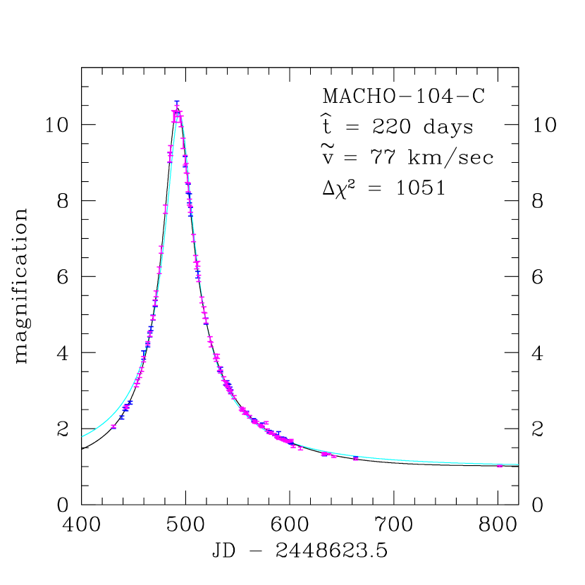
Figure 2: MACHO-104-C light curves normalized to the unlensed flux of the lensed star. The MACHO red and blue data are plotted in magenta and blue, respectively. The black curve is the parallax fit while the cyan curve is the best fit standard microlensing lightcurve. An additional 5 years of data showing no photometric variation are not shown.

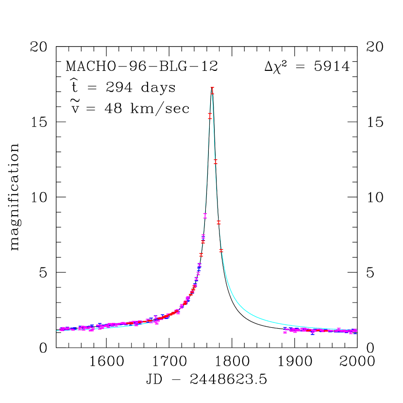
Figure 3: MACHO-96-BLG-12 lightcurve closeup with lightcurves normalized to the unlensed flux of the lensed star. The MACHO red and blue data are plotted in magenta and blue, respectively, and the CTIO data are shown in red. The black curve is the parallax fit while the cyan curve is the best fit standard microlensing lightcurve. An additional 5 years of data showing no photometric variation are not shown.

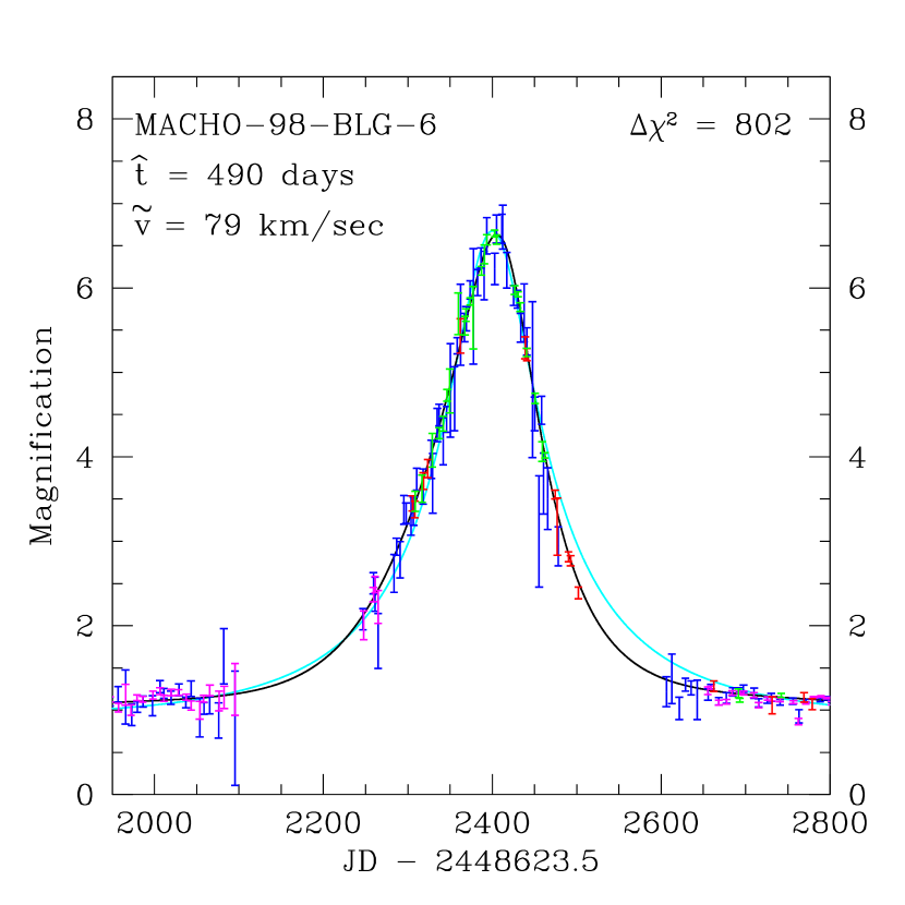
Figure 4: MACHO-98-BLG-6 lightcurve closeup with lightcurves normalized to the unlensed flux of the lensed star. The MACHO red and blue data are plotted in magenta and blue, respectively, the CTIO data are shown in red, and the MPS data are shown in green. The black curve is the parallax fit while the cyan curve is the best fit standard microlensing lightcurve. The gap in the MACHO red data during the day 2280-2650 interval is due to a CCD failure. An additional year of data showing no photometric variation is not shown.

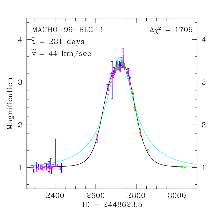
Figure 5: MACHO-99-BLG-1 light curves normalized to the unlensed flux of the lensed star. The MACHO red and blue data are plotted in magenta and blue, respectively, the CTIO data are shown in red, and the MPS data are shown in green. The black curve is the parallax fit while the cyan curve is the best fit standard microlensing lightcurve. An additional 4 years of data showing very little photometric variation are not shown.

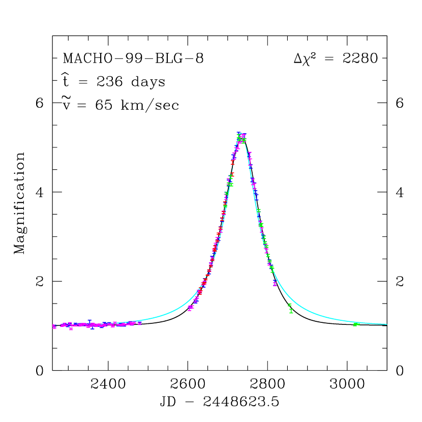
Figure 6: MACHO-99-BLG-8 light curves normalized to the unlensed flux of the lensed star. The MACHO red and blue data are plotted in magenta and blue, respectively, the CTIO data are shown in red, and the MPS data are shown in green. The black curve is the parallax fit while the cyan curve is the best fit standard microlensing lightcurve. An additional 3 years of data showing very little photometric variation are not shown.

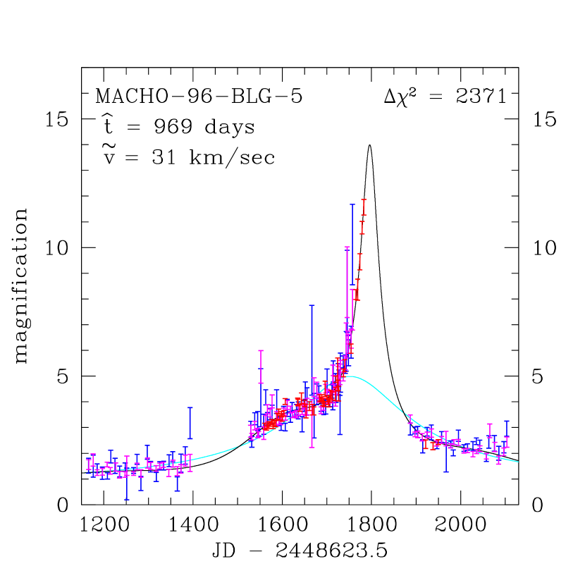
Figure 7: MACHO-96-BLG-5 lightcurves normalized to the unlensed flux of the lensed star. The MACHO red and blue data are plotted in magenta and blue, respectively, and the CTIO data are shown in red. The black curve is the parallax fit while the cyan curve is the best fit standard microlensing lightcurve. An additional 4 years of data showing very little photometric variation are not shown.

The microlensing parallax fits were performed with the MINUIT routine from the CERN Library, and the results for the 6 events that we discuss in this paper are summarized in Table 5. The best fit light curves and data are shown in Figs. 2-7. The significance of the microlensing parallax signal is represented by the parameter $\Delta\chi^{2}$ shown in Table 5 which is the difference between the fit $\chi^{2}$ for a standard microlensing fit with no parallax (i.e.  $\tilde{v}=\infty$) and the best fit presented here. All 28 events with standard microlensing fits (including blending) which indicated $\widehat{t}_{\rm std}>140\,$days where fit with a microlensing parallax model as well, and the 10 events with a microlensing parallax detection with a significance of $\Delta\chi^{2}\geq 50$ are indicated with color in Fig. 1. The four events with $50\leq\Delta\chi^{2}<200$ are MACHO-101-B, MACHO-95-BLG-27, MACHO-98-BLG-1, and MACHO-99-BLG-22, and the six strongest events with $\Delta\chi^{2}\geq 200$ are MACHO-104-C, MACHO-96-BLG-5, MACHO-96-BLG-12, MACHO-98-BLG-6, MACHO-99-BLG-1, and MACHO-99-BLG-8. These 6 events are the primary focus of this paper.

Note that most of the events with $\widehat{t}>200\,$days and all the events with $\widehat{t}>300\,$days have a significant parallax signal. Microlensing parallax is more easily detected in such long events because the Earth’s velocity changes significantly during the event, and because long events are likely to have low $v_{\rm\perp}$ values. There are also a number of events with much shorter timescales that appear to have microlensing parallax signals significant at the $\Delta\chi^{2}\geq 50$ level, but many of these have rather implausible parameters. This is likely to be due to the fact that other effects besides microlensing parallax can perturb the microlensing light curves in ways that can mimic the parallax effect. Examples of this include binary microlensing (see the discussion of MACHO-98-BLG-14 in Alcock et al. 2000a), and the reverse of the parallax effect, the orbital motion of a binary source star (Derue et al., 1999; Alcock et al., 2001a; Griest & Hu, 1993; Han & Gould, 1997), sometimes called the “xallarap” effect. The xallarap effect can be particularly difficult to distinguish from microlensing parallax because a xallarap light curve can be identical to a parallax light curve if the period, inclination, eccentricity, and phase mimic that of the Earth. In practical terms, this is a difficulty only when the xallarap or parallax signal-to-noise is weak so that the fit parameters are poorly determined.

In order to avoid contamination of our microlensing parallax sample with non-parallax microlensing events, we have set a higher threshold for the events that we study in detail in this paper: $\Delta\chi^{2}\geq 200$. The 6 events that pass this threshold are listed in Tables 1 and 5. One of these events, MACHO-104-C, was the first microlensing parallax event ever discovered (Alcock et al., 1995), and the other five events were discovered by the MACHO Alert system. Because of this, they had the benefit of follow-up observations by the MACHO/GMAN Collaboration on the CTIO 0.9m telescope or by the MPS Collaboration on the Mt. Stromlo 1.9m telescope. Four of these five events would have passed the $\Delta\chi^{2}\geq 200$ cut without the follow-up data, but event MACHO-98-BLG-6 only passes the cut because of the MPS follow-up data. This is probably due to a CCD failure that prevented the imaging of this event in the MACHO-Red band during most of the 1998 bulge season.

We have also compared our microlensing parallax fits to binary lens fits for each of these events. The parallax fits are preferred in every case with $\chi^{2}$ improvements of 70.3, 81.6, 1625.8, 227.2, 1957.2, and 1601.3 for events MACHO-104-C, MACHO-96-BLG-5, MACHO-96-BLG-12, MACHO-98-BLG-6, MACHO-99-BLG-1, and MACHO-99-BLG-8, respectively.

4.1 HST Observations of MACHO-96-BLG-5

Event MACHO-96-BLG-5 is both the longest event in our sample, and the event with the faintest source star. In fact, the microlensing parallax fit does not constrain the source star brightness very well. This is due to the faintness of the source, and due to a potential systematic error. The MACHO camera had a CCD upgrade in early 1999 which put a new CCD in the location that views MACHO-96-BLG-5 in the MACHO-Red passband. The new CCD probably had the effect of shifting the effective bandpass to a slightly different central wavelength, and so a slight systematic shift in the photometry of all the stars might be expected to occur with this upgrade. Because the MACHO-96-BLG-5 source is strongly blended with unlensed neighbors, the effect of this slight shift on the microlensing fit parameters can be relatively large because the fitting routine tries to explain all flux variation as resulting from microlensing. The best fit, with this suspect data removed, indicates that only about $12\pm 3$% of the flux associated with the “star” seen in our ground-based images has been microlensed, which would imply that the remaining 88% of the flux must come from unlensed neighboring stars which are within $\sim 1.5$” of the lensed source. Fortunately, we have a set of images from the Hubble Space Telescope’s WFPC2 Camera that can be used to constrain the brightness of the source star more accurately than the fit does.

We had one orbit of HST data taken in the V and I (F555W & F814W) passbands of the WFPC2 Camera through Director’s Discretionary Proposal # 8490, and this can be used to identify the microlensed source star. The first step in this identification process is to determine the centroid of the star that was lensed. This can be accomplished by subtracting two images which have substantially different microlensing magnifications (Alcock et al., 2001b). Since it is only the lensed source star that will appear to vary in brightness, this procedure will yield a point source centered on the location of the lens and source. Of course, the subtraction procedure must take into account the differences in the observing conditions of the two frames, including differences in seeing, pointing, sky brightness and air mass. We have accomplished this with the use of the DIFIMPHOT package of Tomaney & Crotts (1996).

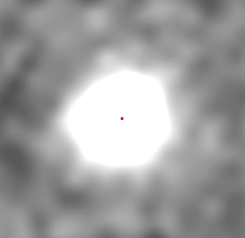
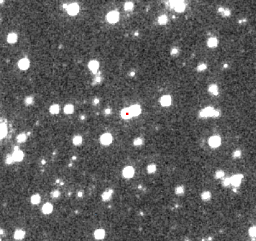
Figure 8: The image on the left is the master difference image as described in the text. It has been registered to the same coordinate system as the F814W HST/WFPC2 image shown on the right. The red marks show the centroid of the variable flux in the master difference image and the location of this centroid when transformed to the coordinate system of the HST data. A single, main sequence bulge star is clearly identified as the lensed source star.

A set of 18 of our best CTIO images were selected to use for this source location task because the CTIO images generally have better seeing than the MACHO images, and because the highest magnification of the source was only observed from CTIO. These 18 images were combined to construct a master reference image which was then subtracted from each individual frame to construct a set of 18 difference images. The difference frames which had a negative flux at the location of our target were inverted, and then all the difference images were combined to make the master difference image shown in Figure 8. The centroid of the excess flux in this master difference image can be determined to better than 0.01.”

In order to identify the lensed source star on the HST images, we must find the correct coordinate transformation to match the ground and HST frames, but this is complicated by the fact that most of the “stars” in the ground-based images actually consist of flux from several different stars that are blended together in the ground-based frames. We have dealt with this in two different ways: first, we used the HST images to select a list of stars that were much brighter than their near neighbors, so that their positions should not be greatly affected by blending in the ground-based images. Then, we convolved the HST data with a 1.2” FWHM Gaussian PSF to simulate the resolution of the ground-based CTIO data. We then analyzed the convolved HST image with the same data reduction software used for the ground-based data. This gave an additional star list from the HST image. Two independent coordinate transformations between the ground-based and HST data were obtained by matching these two stars list to the star list for the ground-based data.

The HST images were dithered, and we combined them with the Drizzle routine (Fruchter & Hook, 1997) prior to the comparison with the ground-based data. The CTIO R-band data were compared to the HST I and V band images as well as sum of the I and V band images. Coordinate transformation were determined to match the CTIO image coordinates to each of these HST images using the bright, isolated stars in the HST images and with the HST images convolved to ground-based seeing. This resulted in a total of 6 different comparisons between the location of the lensed star in the CTIO image and the HST images. All these comparisons yielded the same lens star location on the HST frames to better than 0.02”, and this location coincides with the centroid of the star indicated in Fig. 8. This star was examined carefully in both the V and I images to determine if it could be a blend of more than one star. Model and DAOPHOT generated PSFs were subtracted at the centroid location of the lensed source, but no hint of any additional star was found. This star is very likely to be the source star for the MACHO-96-BLG-5 microlensing event.

The next step in the comparison of the HST and ground-based data is to determine what fraction of the flux of the object identified as a star in the ground-based frames is contributed by the source star identified in the HST images. This task is complicated by the fact that there is no close correspondence between the passbands of the ground based images and those used for the HST data. (This is due to the limitations imposed upon an HST Director’s Discretionary time proposal. We requested prompt images in V and I to confirm the photometric variation implied by the microlensing parallax model, but prompt imaging in R could not be justified. Imaging in R was obtained in a subsequent GO program, and the analysis of these data will appear in a future publication.) Presumably, some combination of the V and I band images would provide a good representation of the R band ground based image.

The determination of the lensed flux fraction was made as follows: Photometry of the V+I combined HST frame was obtained using the IRAF implementation of DAOPHOT (Stetson, 1987) and also using SoDOPHOT. Both of these packages were also used to reduce the HST images which had been convolved to mimic ground based seeing. The total stellar flux of isolated, bright stars was not conserved in these convolved images, so we found it necessary to renormalize the stellar flux in the convolved images to the ratio found for these isolated bright stars. This comparison yielded a flux fraction of 36% for the lensed component of the stellar blend identified as a single star in the ground-based images. We also followed this same procedure for the separate I and V images, and the results for the lensed flux fraction were quite similar as might be expected from the fit results shown in Table 5, which indicate no color dependence for the blending fit parameter. This is likely to be due to the fact that the stars contributing the blended light and the lensed source star are all main sequence stars of similar color which are just below the bulge turn-off.

We must also make a correction for the fact that the source star was still being magnified by the lens when the HST frames were taken. Because the event timescale depends upon the amount of blending that we determine from the HST analysis, it requires an iteration or two to find a fit that predicts the observed brightness of the lensed star in the HST frames. The best fit result is that the lensed source provides 33% of the total flux of the blended object that would be seen in the ground based frames in the absence of any microlensing magnification. At the time of the HST images, the lensing magnification was 1.063 according to this fit.

Finally, we should mention the possibility that the star identified with the lensed source centroid is not, in fact, a single star. The HST images reveal no evidence of a chance superposition of unrelated stars, so this is unlikely. However, it could be that the superposition is not due to chance. Suppose, for example, that the star we’ve identified as the MACHO-96-BLG-5 source is actually the superimposed images of the lens and source. While this is a logical possibility, we will show below that there is no plausible scenario for this to occur because the implied lens mass cannot be made compatible with the observed brightness of the lens plus source.

5 Lens Mass and Distance Estimates

The measurement of the projected speed of the lens, $\tilde{v}$, allows us to relate the lens mass to the lens and source distances

$$M={\tilde{v}^{2}\widehat{t}^{2}c^{2}\over 16G}{D_{s}-D_{\ell}\over D_{\ell}D_{s}}={\tilde{v}^{2}\widehat{t}^{2}c^{2}\over 16G}{1-x\over xD_{s}}\ .$$ (8)

It is often assumed that the distance to the source, $D_{s}$, is already known, at least approximately, so this relation can be considered to give the lens mass as a function of distance. Given the lens distance, one can also work out the lens velocity with respect to the line-of-sight to the source, $v_{\rm\perp}$. But, for some distances, the implied $v_{\rm\perp}$ value can be unreasonably small or large. Thus, with some knowledge of the Galactic velocity distribution, we can work out an estimate for the distance and mass of the lens. This has been done for the MACHO-104-C event using a likelihood method in Alcock et al. (1995). This analysis assumes that the source star resides in the Galactic bulge, which is true for the vast majority of microlensing events seen towards the Galactic bulge. The result of similar analyses for the events presented in this paper are summarized in Table 6 and in Figs. 11-13. However, the microlensing parallax events are selected from a sample of unusually long microlensing events, so it may be that their source star locations are atypical as well. With the data currently available to us, we have two ways to investigate the location of the source stars for our microlensing parallax events. The first is to make use of the direction of projected velocity as determined by the microlensing parallax fit, and the second is to examine the location of the source star in a color-magnitude diagram of nearby stars. Another, perhaps more effective, discriminant between different source populations is radial velocity measurements. Radial velocities for some of the source stars have been measured by Cook et al. (2002), and they have provided us with some preliminary results.

5.1 Source Star Locations

The line-of-sight toward a Galactic bulge microlensing event passes through the Galactic disk, the bulge, and through the Sagittarius (SGR) Dwarf Galaxy behind the bulge. So, all of these are possible locations for the source stars. The variation in the source population/location can affect the inferred properties of the lens in several different ways:

1. Microlensing rate: The microlensing rate per source star is very much lower for foreground Galactic disk stars and very much higher for SGR Dwarf stars than for Galactic bulge stars. Thus, foreground disk stars and SGR Dwarf stars will be under-represented and over-represented, respectively, in samples of microlensed stars when compared to stars in the Galactic bulge.

2. Microlensing parallax detectability: some source star populations such as the foreground Galactic disk and the Sagittarius Dwarf Galaxy give rise to a larger fraction of events with microlensing parallax parameters that can be measured.

3. Source distance: A source at a greater distance than the nominal Galactic bulge distance will usually imply a lower lens mass since $M$ is a decreasing function of $D_{s}$ in eq. (8) (for fixed $x$). Similarly, a smaller $D_{s}$ implies a larger mass.

4. Source velocity: From eq. (7), we see that, for a fixed $\tilde{v}$ value, a smaller $v_{\rm\perp}$ value implies a smaller $D_{s}$ which, in turn, implies a smaller lens mass (for fixed $D_{\ell}$). Smaller $v_{\rm\perp}$ values are expected for lensing of foreground disk sources since the source and lens would both share the Galactic rotation velocity of the Sun.

Several authors who have modeled microlensing parallax events (Mao, 1999; Soszyński et al., 2001; Smith, Mao, & Woźniak, 2001) have suggested that the source stars must be predominantly in the foreground Galactic disk because this makes a small $v_{\rm\perp}$ more likely. A disk source is the only possibility for the OGLE-1999-CAR-1 event since this star is located far from the bulge, but for events towards the Galactic bulge there are several factors that make a foreground disk source star less likely, including a much lower microlensing optical depth and a lower density of source stars. These are discussed in section 5.3, where we find that disk sources that are definitely in the foreground of the bulge at $D_{s}\leq 5\,$kpc are quite unlikely.

5.2 Projected Velocity Distributions

One distinguishing characteristic of microlensing parallax distributions for different source populations is the distribution of the projected velocity, $\tilde{\bf v}$ including both the amplitude, $\tilde{v}$, and the direction $\theta$. We use a Galactic model in which the stars around us are moving with a velocity dispersion of about $30\,$km/sec in both directions normal to the line of sight to the bulge. The Sun rotates at a speed of $+16\,$km/sec faster than the kinematic Local Standard of Rest (LSR) and is moving towards Galactic North at $7\,$km/sec (Dehnen & Binney, 1998). The Galactic disk rotates with an approximately flat rotation curve at $v\simeq 200\,$km/sec, while the Galactic bulge probably has little rotation (Minniti, 1996) and has a velocity dispersion of 80-$100\,$km/sec (Spaenhauer, Jones, & Whitford, 1992; Minniti, 1996; Zoccali et al., 2001). The Sagittarius Dwarf Galaxy is moving at $250\pm 90\,$km/sec in a direction that is only a few degrees away from Galactic North (Ibata et al., 1997).

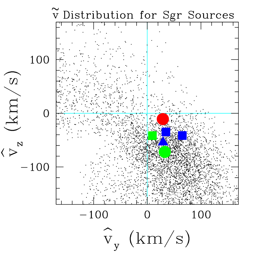
Figure 9: The distribution of $\tilde{\bf v}$ values in Galactic coordinates is shown for simulated microlensing parallax events towards the Galactic bulge for three different source star populations: the Galactic bulge, the foreground Galactic disk, and the Sagittarius Dwarf Galaxy. The large colored dots show the locations of our detected microlensing parallax events. The red circular spot is our best black hole candidate, MACHO-96-BLG-5, and the green circular disk is the other black hole candidate: MACHO-98-BLG-6. The two green spots are the events with source stars that appear to be bulge sub-giants or Sagittarius Dwarf red clump stars. (MACHO-99-BLG-1 is the other). The blue squares are the bulge red clump source star events, and the blue triangle is MACHO-98-BLG-8 which has a red giant source and is probably also in the bulge.

The different velocity distributions of these source and lens populations lead to different expectations for the measured $\tilde{\bf v}$ distributions for events from different source star populations. However, the observed $\tilde{\bf v}$ distribution is strongly affected by selection effects since only a small fraction of microlensing events have detectable parallax signals. These selection effects can be difficult to precisely quantify because of the fact that much of the data taken for these events comes from follow-up programs with observing strategies that can be subjective and difficult to model. Therefore, instead of attempting a detailed simulation of the actual observing conditions, we investigate the $\tilde{\bf v}$ distribution using a “toy model” of a microlensing survey and follow-up program. ((Buchalter & Kamionkowski, 1997) also performed simulations of microlensing parallax events in a somewhat different context.) We assume a disk velocity dispersion of $30\,{\rm km/s}$ in each direction, with a flat rotation curve of $200\,{\rm km/s}$ and a bulge velocity dispersion of $80\,{\rm km/s}$ with no bulge rotation, and the density profiles are a standard double-exponential disk and a barred bulge as in Han & Gould (1996). We assume that events are observed for 7 months per year by a microlensing survey system that makes photometric observations with 5% accuracy every 3 days. Once an event is magnified by at least 0.5 magnitudes, daily follow-up observations start with an accuracy of 1% for each day. This simulated data are then fit with a standard, no-parallax microlensing model, and the $\Delta\chi^{2}$ is determined. (Since we have not added noise to the light curves, the fit $\chi^{2}=0$ when there is no microlensing parallax signal.) Events with $\Delta\chi^{2}\geq 200$ are considered microlensing parallax detections, and the $\tilde{\bf v}$ values for these simulated detected events are shown in Figure 9. This figure uses Galactic coordinates in which the $y$-axis is the direction of Galactic disk rotation, and the $z$-axis is Galactic North.

A striking feature of Figure 9 is that all six of our strong microlensing parallax events have $\tilde{\bf v}$ in the same quadrant with positive $\tilde{v}_{y}$ and negative $\tilde{v}_{z}$. This is the region that is preferred for both bulge and SGR source stars, but not for foreground disk sources. In our simulations, 65% of the detectable SGR source events, and 50% of the detectable bulge sources, but only 29% of foreground disk sources lie in this quadrant.

One selection effect that affects each plot is that events with $\tilde{\bf v}$ roughly parallel to the ecliptic plane are easier to detect than events where $\tilde{\bf v}$ is approximately perpendicular to the ecliptic plane. This effect favors the positive $\tilde{v}_{y}$-negative $\tilde{v}_{z}$ and negative $\tilde{v}_{y}$-positive $\tilde{v}_{z}$ quadrants. The reason for this is that the Earth’s orbital motion only affects $u(t)$ near peak magnification when $\tilde{\bf v}$ is perpendicular to the ecliptic plane, but the orbital motion affects $u(t)$ for a longer period of time when it is parallel to $\tilde{\bf v}$.

For the bulge sources, there is a preference for positive $\tilde{v}_{y}$ motion because disk lens stars are passing inside of us at a higher angular velocity. If the source stars are rotating with us, as would be the case for disk sources in the foreground of the bulge, then the rotation is common to the source, lens and observer, and it has no effect. A smaller systematic effect occurs in the disk source case because the Sun is moving about $16\,$km/sec faster than the mean stellar motion around us. Thus, there is a slight enhancement of the abundance of negative $\tilde{v}_{y}$ events.

For SGR source stars, signal of the SGR proper motion toward the Galactic North can clearly be seen in the strong concentration of events at negative $\tilde{v}_{z}$ and positive $\tilde{v}_{y}$. (Since $\tilde{\bf v}$ is a lens$-$source velocity, the $\tilde{\bf v}$ signal is in the opposite direction of the SGR motion.) For bulge lenses, the $250\,$km/sec velocity is reduced to $90\,$km/sec by the projection effect, and for the disk lenses that make up the bulk of microlensing parallax sample for SGR sources, the typical $\tilde{v}_{z}$ is $-50\,$km/sec or so. For SGR sources, and disk lenses, the combination of SGR proper motion and disk rotation put the majority of $\tilde{\bf v}$ values in the positive $\tilde{v}_{y}$-negative $\tilde{v}_{z}$ quadrant where the alignment with the ecliptic plane makes the parallax effect easy to detect.

5.3 Microlensing Parallax Selection Effects

For comparison between the different source populations, it is necessary to consider several different selection effects. First, the microlensing rate for SGR sources behind our fields is a factor of $\sim 6$ larger than for bulge source stars (Cseresnjes & Alard, 2001), and the fraction of SGR events with detectable microlensing parallax signals is a factor of 3 larger for sources in SGR than for bulge sources. Thus, it would appear that the probability of detecting a microlensing parallax event for a SGR source is a factor of $\sim 20$ higher than for a bulge source (assuming that the sources are bright enough for reasonably accurate photometry). Of course, Galactic bulge sources are much more numerous, so microlensing parallax events with Galactic bulge source stars are likely to be more numerous than events with SGR source stars by an amount that is difficult to estimate. We consider this in detail in Section 5.4 when we present the source star color-magnitude diagrams.

It is quite difficult to distinguish Galactic bulge stars from stars in the inner Galactic disk because they are at similar distances and their velocity distributions overlap. In fact, this distinction is likely to be somewhat artificial because the two components are likely to have merged due to their mutual gravitational interactions. Therefore, we will limit our consideration of foreground disk sources to stars with a distance $<5\,$kpc. For stars at $5\,$kpc distance at a Galactic latitude of $b=-3^{\circ}$, the microlensing rate is a factor of about $\sim 40$ lower than for Galactic bulge stars. (The optical depth is only a factor of $\sim 20$ lower because of the longer time scales of disk-disk lensing events.) The physical density of disk stars is about an order of magnitude lower than the density of bulge stars, but there is also a volume factor that reduces the number of disk stars per unit distance modulus and solid angle by a factor of 4 at $5\,$kpc. The product of these factors yields a net suppression factor of $1/1600$ for disk star lensing events for a fixed source star absolute magnitude.

This suppression factor must be multiplied by two enhancement factors. First, our simulations indicate that the chances of detecting a microlensing parallax signal are about a factor of 5 larger for disk sources than for bulge source stars. This increases the suppression factor to $\sim 1/320$. There is an additional enhancement factor due to the fact that the foreground disk stars are intrinsically fainter and the stellar luminosity function rises for fainter stars, but the difference between the disk stars at $5\,$kpc and the bulge stars at $8\,$kpc is only 1 magnitude. From Holtzman et al. (1998) we see that this factor is at most $\approx 10$ if we select a source magnitude such that is 1-2 magnitudes above the bulge main sequence turnoff. For magnitudes that correspond to bulge main sequence stars, it is less than a factor of two. Thus, we expect disk stars (with $D<5\,$kpc) to contribute less than 1% of the total number of detectable microlensing parallax events, except for source stars that are 1-2 magnitudes above the bulge main sequence turn-off where they might account for as many as 3% of the microlensing parallax events with bulge source stars.

Inner disk stars at $D>5\,$kpc will be accounted for by allowing their velocities to contribute to the assumed bulge velocity distribution. In fact, such inner disk stars are generally not excluded from star samples that are used to measure the bulge proper motion (Spaenhauer, Jones, & Whitford, 1992; Zoccali et al., 2001). We will, therefore, classify all stars in the vicinity of the bulge ($5\,{\rm kpc}<D_{s}<11\,{\rm kpc}$) as bulge stars. Instead of trying to distinguish different, but overlapping, populations of source stars, we consider a single model including all these stars.

Stars on the far side of the disk have velocities that make it very unlikely to see the microlensing parallax effect, while foreground disk stars are unlikely to be microlensed at all. Therefore, the SGR dwarf provides the only “non-bulge” population of potential source stars that we will consider in the remainder of this paper.

5.4 Color Magnitude Diagrams

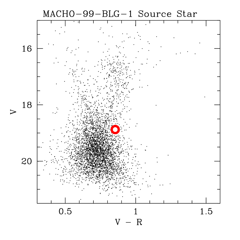
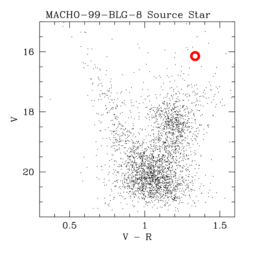
Figure 10: Color-Magnitude diagrams from MACHO data are shown for all the detected stars within a 2 arc minute circle around each of our microlensing parallax events. The red circles indicate the location of the lensed source star, assuming the blending implied by the microlensing parallax fits.

Fig. 10 shows color-magnitude diagrams for all the stars within 2 arc minutes around each of our microlensing parallax source stars, with the lensed source indicated by a red circle. It is necessary to use different color magnitude diagrams for each event because of the large variation in reddening between different fields. By plotting only the stars within 2 arc minutes of our targets, we have minimized the variation in reddening.

These CM diagrams indicate that the MACHO-104-C and MACHO-96-BLG-12 source stars are located in the bulge red clump region, which means that they are likely to reside in the Galactic bulge. The MACHO-99-BLG-8 source star is more luminous than the red clump and is likely to be a bulge giant. Cook et al. (2002) find a radial velocity of $v_{r}=195\pm 2\,{\rm km/s}$ which confirms the bulge interpretation for this event. The MACHO-96-BLG-5 source star appears to be fainter than virtually all of the other stars in its CM diagram. This is a consequence of the extreme crowding of these Galactic bulge fields. The density of bright main sequence stars is $\sim 2$ per square arc second, so main sequence stars are not individually resolved in these crowded Galactic fields. Instead, it is groups of unresolved main sequence stars that are identified as single stars, and it is these unresolved blends of multiple stars that make up the majority of the fainter objects identified as stars in these images. The majority of microlensed source stars in the Galactic bulge are blended main sequence stars like the MACHO-96-BLG-5 source, but the microlensing parallax signal is easier to detect for brighter source stars.

The source stars for events MACHO-98-BLG-6 and MACHO-99-BLG-1 appear to be on the bulge sub-giant branch of the color magnitude diagram. They have a similar color to bulge red clump stars, but they are about 2 magnitudes fainter. This suggests that they could be red clump stars $\sim 14\,$kpc behind the bulge in Sagittarius (SGR) Dwarf Galaxy. This is about the only location on the color magnitude diagram were we might expect to see microlensing of SGR source stars, because SGR red clump stars are probably the only abundant type of SGR stars that are brighter than the bulge main sequence stars that set the confusion limit. This SGR source interpretation appears to gain support from the location of these events in Fig. 9 which indicates that their parallax velocities are among the ones most consistent with Sagittarius Dwarf kinematics.

A rough estimate of the probability of detecting microlensed SGR source stars can be made by noting that SGR Dwarf RR Lyrae stars are about 2.6% as numerous as bulge RR Lyrae in the MACHO fields (Alcock et al., 1997a). In a microlensing parallax sample, we should expect SGR source stars to be enhanced by a factor of $\sim 20$, but we must also include both bulge sub-giants and giants in the comparison with the SGR red clump giants. This would reduce the fraction of SGR events by a factor two or so. This would suggest that we might expect that for every 4 microlensing parallax events with bulge giant or sub-giant source we could expect one SGR giant source star event. On the other hand, the ratio of red clump stars to RR Lyrae is likely to be higher for SGR stars than for Galactic bulge stars because of the lower metalicity of SGR, so we might expect fewer SGR events than this RR Lyrae comparison would suggest.

These considerations suggest that we should take the SGR source star hypothesis seriously for these events. However, Cook et al. (2002) used the Keck HIRES spectrograph to obtain spectra of the source stars for these events, and they find radial velocities of $v_{r}=-65\pm 2\,{\rm km/s}$ and $v_{r}=64\pm 2\,{\rm km/s}$ for MACHO-98-BLG-6 and MACHO-99-BLG-1, respectively. This is not consistent with the SGR radial velocity (Ibata et al., 1997) of $v_{r}=140\pm 10\,{\rm km/s}$, and they are about $2\sigma$ away from the expectation for a disk source star (Wielen, 1982). Thus, these events are most likely to have bulge sub-giant source stars.

5.5 Likelihood Distance and Mass Estimates

Another, somewhat more general, constraint on $x$ and $M$ can be obtained if we make use of our knowledge of the velocity distributions of the source and lensing objects, since the likelihood of obtaining the observed value of $\tilde{\bf v}$ is a strong function of the distance to the lens. Note that this assumes that stellar remnant lenses have a velocity and density distribution that is similar to that of observed stellar populations. For neutron stars, this might be a questionable assumption because many neutron stars are apparently born with a large “kick” velocity. However, for black holes, the evidence indicates that significant kick velocities are rare (Nelemans, Tauris, & van den Heuvel, 1999). As an example of such an analysis, let us suppose that the disk and bulge velocity dispersions were negligible relative to the Galactic rotation velocity. Then, for disk lenses we would obtain the relation $\tilde{v}=200D_{\ell}/(D_{s}-D_{\ell})\,{\rm km/s}$ implying a lens distance of $D_{\ell}=D_{s}\tilde{v}/(\tilde{v}+200\,{\rm km/s})$. In reality, the random motions of both disk and bulge stars broaden this relationship somewhat, but we can still obtain a useful constraint.

Given the observed $\tilde{\bf v}$, we obtain a likelihood function

$$L(x;\tilde{\bf v})\propto\sqrt{x(1-x)}\,\rho_{L}(x)\,\tilde{v}(1-x)^{3}\int f_{S}({\bf v}_{S})\,f_{L}((1-x)({\bf v}_{\odot}+\tilde{\bf v})+x{\bf v}_{S})\,d{\bf v}_{S},$$ (9)

where $\rho_{L}$ is the density of lenses at distance $x=D_{\ell}/D_{s}$, and the integral is over combinations of source and lens velocities giving the observed $\tilde{\bf v}$. ${\bf v}_{S}$ and ${\bf v}_{L}=(1-x)({\bf v}_{\odot}+\tilde{\bf v})+x{\bf v}_{S}$ are the 2-D source and lens velocity distribution functions (normalized to unity). We assume the same Galactic parameters as in our $\tilde{v}$ simulations above: a disk velocity dispersion of $30\,{\rm km/s}$ in each direction, a flat disk rotation curve of $200\,{\rm km/s}$, and a bulge velocity dispersion of $80\,{\rm km/s}$ with no bulge rotation. The density profiles are a standard double-exponential disk and a Han & Gould (1996) barred bulge. For all events, the source is assumed to reside in the bulge, while the lens may be in the disk or the bulge. But for events MACHO-98-BLG-6 and MACHO-99-BLG-1, we also consider the possibility of a SGR Dwarf source star with the lens in the disk or bulge, although this now appears to be ruled out (Cook et al., 2002).

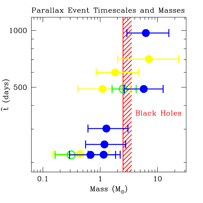
Figure 14: This plot shows $M$ vs. $\widehat{t}$ for the 10 events with $\widehat{t}>140\,$ days with $1\sigma$ error bars for the mass estimates. All events with formally significant detections of microlensing parallax are shown, but parallax signal for the events indicated in yellow is weak enough that the detection is not considered to be definitive. The green open symbols indicate the predicted lens masses for MACHO-98-BLG-6 and MACHO-99-BLG-1 if their source stars were in the SGR Dwarf Galaxy, a possibility that appears to be contradicted by their spectra.

The resulting likelihood functions for $D_{\ell}$ is shown as the long-dashed curves in Figs. 11-13, and these are insensitive to specific parameter choices. These likelihood functions also provide a means for estimating the lens masses via the relation (8), which is also plotted in Figs. 11-13. Fig. 14 shows how the mass estimates correlate with the best fit event timescale for the six high signal-to-noise microlensing parallax events as well as four other events of lower signal-to-noise. (The lower signal-to-noise event with the highest mass is MACHO-99-BLG-22/OGLE-1999-BUL-32 which has been presented as a black hole candidate by Mao et al. 2001.)

One common way to interpret likelihood functions is the Bayesian method, in which the lens mass (or distance) probability distribution is given by the likelihood function times a prior distribution, which represents our prior knowledge of the probability distribution. In our case, the likelihood function represents all of our knowledge about the lens mass and location, so we select a uniform prior. With a uniform prior, the likelihood function becomes the probability distribution and we are able to calculate the lens mass confidence levels listed in Table 6. This table also includes lens mass confidence levels for models that differ from the preferred model in order to show how the mass estimates depend upon the amount of blending (for MACHO-96-BLG-5) and on whether the source star resides in the Galactic bulge or the SGR Dwarf. Note that the uncertainty in the mass estimates is smaller for SGR Dwarf sources due to the small velocity dispersion of the SGR Dwarf and the smaller range of likely lens distances.

5.6 Constraints on Main Sequence Lenses

If we assume that the lens stars are main sequence stars, then we can obtain an additional constraint on their distances and masses by comparing the brightness of a main sequence star, of the implied mass, to the upper limit on the brightness of the lens star. We have assigned a conservative upper limit on the V-band brightness of each lens star based upon the available photometry and microlensing parallax fits listed in Table 5. In the case of MACHO-96-BLG-5, the upper limit is particularly stringent because it is based upon HST observations. Note that if we assign some of the flux of the star identified in the HST images to the lens star instead of the source, the best fit $\widehat{t}$ will increase almost linearly with the inverse of the source star flux. This causes the lens mass estimate to increase as $\sim\widehat{t}^{2}$. Since stellar luminosity varies as a high power of the mass, a main sequence lens will be more strongly ruled out.

In order to apply these constraints to the likelihood functions for the mass and distances of the lens stars, we have multiplied the likelihood function by the Gaussian probability that the lens brightness exceeds the upper limit on the brightness of lens star. If a main sequence lens star would be fainter than the observed maximum brightness, there is no modification of the likelihood function. This gives the short-dashed likelihood curves shown in Figs. 11-13. These results are insensitive to our assumed $L\propto M^{4}$ mass-luminosity relation. The assumed maximum lens brightnesses are $V=19.88$, $20.57$, and $16.92$ for events MACHO-96-BLG-12, MACHO-98-BLG-6, and MACHO-99-BLG-8, respectively. These are based upon the amount of blending allowed by the fit, and each of these has an assumed 25% uncertainty which is also based upon the fit. For MACHO-96-BLG-5, the maximum lens brightness is $V=23.63$, with an assumed 50% uncertainty. For MACHO-104-C, and MACHO-99-BLG-8, the best fit has very little blended flux: $V=22.33$, and $23.08$, respectively. But, in both cases, the uncertainty in the blended flux is five times the best fit value.

The properties of the most likely main sequence lens models are given in Table 7, which is discussed in more detail in section 6.2. An important parameter in this table is the predicted lens-source separation in June, 2003, when they might plausibly be observed by HST. This can be calculated from the lens-source proper motion which is related to the projected velocity by $\mu=\tilde{v}(D_{s}-D_{\ell})/(D_{s}D_{\ell})$.

5.7 Stellar Remnant Lenses and Black Hole Candidates

The mean mass estimate for the six microlensing parallax events is $2.7\rm{M_{\odot}}$. Five of the six have best fit masses $>1\,\rm{M_{\odot}}$, and two of the events, MACHO-96-BLG-5 and MACHO-98-BLG-6, have best fit masses $>3\rm{M_{\odot}}$. This makes them black hole candidates because the maximum neutron star mass is thought to be $\sim 2\rm{M_{\odot}}$ (Akmal, Pandharipande, & Ravenhall, 1998). The 95% confidence level lower limits on the masses of these lenses are $1.64\rm{M_{\odot}}$ and $0.94\rm{M_{\odot}}$, respectively, while the 90% confidence level lower limits are $2.3\rm{M_{\odot}}$ and $1.9\rm{M_{\odot}}$. A main sequence star lens at the lower limit mass is strongly excluded in the case of MACHO-96-BLG-5 because of the constraint on the lens brightness from HST images. However, a main sequence lens with a mass at the 95% confidence limit is not quite excluded for MACHO-98-BLG-6. The masses that have been measured for neutron stars are close to the Chandrasekhar mass, $M_{NS}=1.35\pm 0.04\rm{M_{\odot}}$ (Thorsett & Chakrabarty, 1999), which is excluded at better than 95% confidence for MACHO-96-BLG-5 and better than 90% confidence for MACHO-98-BLG-6. Thus, both MACHO-96-BLG-5 and MACHO-98-BLG-6 are both black hole candidates, but there is a small chance that MACHO-98-BLG-6 could be a neutron star or even a main sequence star.

In addition to these black hole candidates, three of the remaining four microlensing parallax events have best fit masses $>1\rm{M_{\odot}}$. For MACHO-104-C and MACHO-96-BLG-12, main sequence lens are disfavored, but not ruled out. MACHO-99-BLG-8 appears to be blended with a relatively bright source, so a main sequence lens of $M\lower 2.15277pt\hbox{$\;\buildrel>\over{\sim}\;$}1\rm{M_{\odot}}$ is a possibility. As we explain below, with HST imaging it will be straightforward to detect the lenses if they are main sequence stars. If HST images fail to detect the lens stars, then we can show that the lenses are almost certainly stellar remnants.

5.8 Likelihood Analysis with a Mass Function Prior

The Likelihood analysis presented in Section 5.5 attempts to estimate the distance to the lens based upon the measured value of the projected velocity, $\tilde{\bf v}$, and then the lens mass is determined from eq. 8. If the lens mass function, $dn/dM=\phi(M)$, is known, then it is possible to use the measured $\widehat{t}$ value to make a more accurate estimate of the lens mass as advocated by Agol et al. (2002). The likelihood function, eq. 9, can be modified by multiplying by $\delta(\widehat{t}-\widehat{t}_{m})M^{1/2}\phi(M)dM$ and integrating over $M$, where $\widehat{t}_{m}$ is the measured value of $\widehat{t}$. The factor of $M^{1/2}$ is the contribution of the lens mass to the lensing cross section, which is proportional to $R_{E}$. The integral over $\delta(\widehat{t}-\widehat{t}_{m})dM$ gives an additional factor of $M$. Thus, the likelihood analysis presented in Section 5.5 is equivalent to assuming a mass function of $\phi(M)\propto M^{-1.5}$.

A more conventional mass function for the Galactic bulge is a broken power law initial mass function (Kroupa, 2002) with $\phi(M)\propto M^{-1.3}$ for $0.03{\rm{M_{\odot}}}\leq M\leq 0.8\rm{M_{\odot}}$, and $\phi(M)\propto M^{-2.35}$ for $0.8{\rm{M_{\odot}}}\leq M\leq 100\rm{M_{\odot}}$. However, the stars with $M>1.0\rm{M_{\odot}}$ will generally have ended their main sequence lifetimes and have become stellar remnants after significant mass loss. Following Fryer & Kalogera (2001), we can assume that all stars with an initial mass greater than a particular cutoff mass, $M_{i}>M_{\rm BH}$ become black holes. We take $M_{\rm BH}=20\rm{M_{\odot}}$ (Fryer, 1999; Fryer & Kalogera, 2001). Similarly, we assume that all stars with $8{\rm{M_{\odot}}}\leq M_{i}<M_{\rm BH}$ become neutron stars, and all stars with $1.0{\rm{M_{\odot}}}<M_{i}<8{\rm{M_{\odot}}}$ become white dwarfs. The mass functions of the stellar remnants are assumed to be Gaussians with mean masses of $0.6\rm{M_{\odot}}$, $1.35\rm{M_{\odot}}$, and $8\rm{M_{\odot}}$ for white dwarfs, neutron stars, and black holes respectively. The Gaussian sigmas are $0.15\rm{M_{\odot}}$, $0.04\rm{M_{\odot}}$, and $2.5\rm{M_{\odot}}$, respectively. These are consistent with the measured mass functions (Bergeron, Saffer, & Liebert, 1992; Bergeron, Leggett, & Ruiz, 2001; Thorsett & Chakrabarty, 1999; Bailyn, Jain, Coppi, & Orosz, 1998), although the difficulty of directly observing old stellar remnants assures that the observed samples are incomplete. With this mass function, black holes would account for 3.7% of the Galaxy’s stellar mass.

A Bayesian analysis based upon this mass function gives a probability of 93% that the MACHO-96-BLG-5 lens is a black hole and a probability of 69% that the MACHO-98-BLG-6 lens is a black hole. The probability of at least one black lens is 98%. This analysis may underestimate the black hole probability because the assumed mass function cannot account for the large number of long timescale microlensing events. An initial IMF that is slightly shallower than the Salpeter slope, $\phi(M)\propto M^{-2.0}$, might be appropriate if most of the stars in the Galaxy were formed in denser or more metal poor regions than is typical for present day star forming regions (Figer et al., 1999; Smith & Gallagher, 2001). With this mass function and with $M_{\rm BH}=20\rm{M_{\odot}}$, black holes would account for 12% of the Galaxy’s stellar mass. When we repeat the likelihood analysis with this mass function, we find black hole probabilities of 97% for MACHO-96-BLG-5 and 88% for MACHO-98-BLG-6. The probability of at least one black hole lens with this mass function is 99.7%. If we retain the Salpeter IMF slope, and increase $M_{\rm BH}$ to $40\rm{M_{\odot}}$, then the black hole probabilities for MACHO-96-BLG-5 and MACHO-98-BLG-6 drop to 82% and 43%, respectively. However, such a mass function probably cannot explain the excess of long timescale events.

We should note that these probabilities are substantially larger than those reported in a similar analysis in a preprint by Agol et al. (2002). This was due to a likelihood function calculation error by Agol et al. (2002). When this error is corrected, their results are quite similar to those presented here (Agol, private communication).

6 Follow-up Observations

The detection of the microlensing parallax effect allows us to make a lens mass estimate that is accurate to about a factor of two, and to identify the black hole candidates. However, these estimates are not accurate enough to determine the black hole mass function, and they do not allow the unambiguous identification of neutron star or white dwarf lenses. However, follow-up observations with higher resolution instruments hold the promise of much more precise determinations of the lens masses.

6.1 Interferometric Follow-up

The most ambitious of microlensing event follow-up plans involve interferometric instruments such as the Keck and VLT interferometers (Delplancke, Górski & Richichi, 2001) and the Space Interferometry Mission (SIM) (Boden, Shao, & van Buren, 1998). The most spectacular confirmation of a black hole event would be to measure the image splitting which is given by

$$\phi_{\rm sep}=2\theta_{E}\sqrt{1+u^{2}/4}\ ,$$ (10)

where $\theta_{E}$ is the image separation and $u$ is given by eq. (4). For MACHO-96-BLG-5, we have $\theta_{E}=9.8\,$mas if the lens is at the distance preferred by the likelihood analysis. This compares to the $5\,$mas diffraction limit of an interferometer with a $100\,$m baseline operating at a wavelength of $2\,\mu$m, such as the Keck or VLT Interferometers. In fact, these instruments are expected to be able to measure image splittings as small as $\sim 30\,\mu$as (Delplancke, Górski & Richichi, 2001). Such measurements would allow a direct measurement of the lens mass:

$$M={\tilde{v}\widehat{t}\theta_{E}c^{2}\over 8G}\ .$$ (11)

The most challenging aspect of such measurements is the faintness of source stars such as the MACHO-96-BLG-5 source, which is close to the (rather uncertain) magnitude limit of the VLT Interferometer (Delplancke, Górski & Richichi, 2001).

Even if the images cannot be resolved, it may be possible to measure the deflection of the image centroid (Hog, Novikov, & Polnarev, 1995; Miyamoto & Yoshi, 1995; Walker, 1995) which is given by

$$\Delta\phi=\left({u^{2}+3\over\sqrt{u^{2}+4}}-u\right)\theta_{E}\ .$$ (12)

This can be measured by a very accurate astrometry mission such as SIM (Boden, Shao, & van Buren, 1998; Paczyński, 1998; Gould, 2000). Once again, however, the MACHO-96-BLG-5 source is a rather faint target for SIM, but in this case, the measurement is not so difficult because the amplitude of the centroid motion is very much larger than SIM’s sensitivity limit.

If it should turn out that some of the more massive lenses are located very close to us, then it might be possible to directly observe the lensed images with HST. This is a realistic possibility for the MACHO-99-BLG-22/OGLE-1999-BUL-32 event (Mao et al., 2001) because its $\tilde{\bf v}$ value is in the opposite quadrant from the events studied in this paper. This gives a likelihood function with two peaks: one at a distance of $\sim 500\,$pc for a lens in the disk and one at a distance of $\sim 6\,$kpc for a bulge lens (Bennett et al., 2002). The bulge lens solution predicts a mass of a few $\rm{M_{\odot}}$, but the disk lens solution predicts a mass of $>100\rm{M_{\odot}}$ and a lensed image separation of $\sim 0.1$.”

6.2 Lens Detection and Source Proper Motion

Another method can be used to make a direct determination of the lens mass for a bright lens star. If the lens can be detected and the relative proper motion of the lens with respect to the source is measured, then it is also possible to determine the lens mass from the proper motion and microlensing parallax parameters with the following formula:

$$M={\tilde{v}\widehat{t}^{2}\mu c^{2}\over 16G}\ ,$$ (13)

where $\mu$ is the relative lens$-$source proper motion. This technique has the advantage that the proper motion measurements can be made many years after the peak magnification of the microlensing event. The lens-source separation can reach the 50-100 mas range within 5-10 years. Table 7 shows the predicted separations and lens brightness contrasts for our six strong microlensing parallax events. The columns are (1) the MACHO event name, (2) the lens mass with $1\sigma$ errors, (3) a likely lens mass, $M_{rmMS}$, if the lens is on the main sequence, (4) the lens distance, $D_{\ell-{\rm MS}}$ for a lens of mass $M_{rmMS}$, (5) the predicted lens-source separation in June, 2003, (6) the apparent V magnitude of the lenses, and (7-11) the predicted contrast between the lens and source brightness in the UBVI bands. Positive $\Delta$-mags. imply that the source is brighter than the lens, so lens detection is easiest for events that have small or negative $\Delta$-mag. values. With the exceptions of MACHO-96-BLG-5, which doesn’t have a viable main sequence lens model, all of the other lens stars should be detectable if they are not stellar remnants.

When the lens can be detected, it should also be possible to constrain the unlensed brightness of the source star, which will reduce the error bars on $\widehat{t}$. Also, it should be possible to get very accurate measures of the relative proper motion, $\mu$, as the lens moves further from the source. Thus, the ultimate limits on the masses of the lenses may come from the uncertainties in the $\tilde{v}$ values, which range from $2-10\,$%.

When the lenses are undetectable, it should still be possible to measure the proper motion of the source star with HST images separated by $\sim 5$ years. The proper motion can only be measured with respect to the average of other, nearby stars because extra-galactic reference sources are not easily identified in these crowded Galactic bulge fields (Spaenhauer, Jones, & Whitford, 1992; Zoccali et al., 2001). Proper motion measurements of the microlensed source stars would allow us to remove one degree of freedom from our likelihood analysis and reduce the uncertainty in the implied lens distances and masses. The proper motion distribution of the stars in the same field will also allow us to test the Galactic models that are used for the likelihood analysis, and so this should reduce the systematic uncertainties in the lens distance and mass estimates.

7 Discussion and Conclusions

We have performed microlensing parallax fits on the Galactic bulge events detected by the MACHO Collaboration with timescales of $\widehat{t}\geq 140\,$days, and found six events with highly significant detections of the microlensing parallax effect. Our analysis of the velocity distributions expected for parallax microlensing events from different source star populations suggests that source stars in the SGR Dwarf Galaxy might contribute to the detectable microlensing parallax events, and inspection of the source star color-magnitude diagrams indicates that two of our microlensing parallax events have source stars which could be SGR Dwarf red clump stars. However, radial velocity measurements (Cook et al., 2002) indicate that they are probably bulge sub-giant stars.

A likelihood analysis has been employed to estimate the distance and masses of the lenses, and this indicates an average mass for our six lenses of $2.7\,\rm{M_{\odot}}$. Two of the lenses have masses large enough to imply that they are probably massive stellar remnants: The mass estimates for the MACHO-96-BLG-5 and MACHO-98-BLG-6 lenses are $M/\rm{M_{\odot}}=6{+10\atop-3}$ and $M/\rm{M_{\odot}}=6{+7\atop-3}$, respectively, which implies that both are likely to be black holes. Together with MACHO-99-BLG-22/OGLE-1999-BUL-32 (Mao et al., 2001), these are the first black hole candidates that are truly black since we have not seen any radiation from matter that is gravitationally bound to the black hole.

Our likelihood analysis differs from that of Agol et al. (2002) in that we compute the likelihood for the measured $\tilde{\bf v}$ value whereas Agol et al. (2002) attempt to compute the likelihood of the measured values of $\widehat{t}$ as well as $\tilde{\bf v}$. However, this requires that we input the mass function of the lenses, and this has never been measured for a complete sample of stellar remnants. Thus, the method of Agol et al. (2002) can give misleading results if the input mass function is not correct. Nevertheless, the results of such an analysis are consistent with the results that we have presented here. (Note that the preprint version of Agol et al. (2002) claimed an inconsistency with our results, but this was due to an error in the computation of the likelihood function (Agol, private communication).) For the MACHO-99-BLG-22/OGLE-1999-BUL-32 event, the method of Agol et al. (2002) does give potentially misleading results, however, because the shape of the Likelihood function for this event makes the results quite sensitive to the assumed black hole mass function (Bennett et al., 2002), which is, of course, unknown.

Similar events detected in the next few years may yield lens masses that are measured much more precisely due to follow-up observations from ground-based (Delplancke, Górski & Richichi, 2001) and space-based (Gould, 2000) interferometers. This will allow an unambiguous determination of the abundance and mass function of black hole and neutron star stellar remnants, although it may be difficult to determine if $\sim 2\,\rm{M_{\odot}}$ objects are black holes or neutron stars. At present, there are three black hole microlens candidates in the sample of 321 microlensing events that was the starting point for this paper (although MACHO-99-BLG-22 is only identified as a strong black hole candidate when OGLE data are included in the analysis (Mao et al., 2001; Bennett et al., 2002)). This is about 1% of the events, but far more than 1% of the total contribution to the microlensing optical depth. This suggests that the fraction of our Galaxy’s stellar mass that is in the form of black holes may be significantly larger than 1%, which might help to explain the observed excess of long timescale microlensing events. However, we have not made an accurate determination of our microlensing event detection efficiency for this data set, and the detection efficiency is certainly larger for long timescale microlensing events than for short events. It is also possible that one of these three lenses may not be a black hole, and so these microlensing results may still be consistent with models which predict that of order 1% of the Milky Way’s stellar mass should be in the form of black holes (Brown & Bethe, 1994; Fryer & Kalogera, 2001; Gould, 2000). If all three of these events are truly due to black hole lenses, then a black hole mass fraction as high as $\sim 10$% might be preferred. These results appear to indicate that most stellar mass black holes do not reside in the X-ray binary systems where they are most easily observed (Bailyn, Jain, Coppi, & Orosz, 1998).

Figure 11: The mass vs. distance relations (solid curves) for our candidate black hole lenses are shown along with the likelihood functions (long dashed curves) computed assuming a standard model for the Galactic phase space distribution. The source star is assumed to reside in the bulge for both events. The implied best fit masses are $M=6{+10\atop-3}\rm{M_{\odot}}$ for the MACHO-96-BLG-5 lens and $M=6{+7\atop-3}\rm{M_{\odot}}$ for the MACHO-98-BLG-6. The 95% confidence level lower limits on the masses are $1.6\rm{M_{\odot}}$ and $0.94\rm{M_{\odot}}$ respectively. The short dashed curves delineate the portion of the likelihood functions that is allowed when the lens is assumed to be a main sequence star. The ratio of the area below this portion to the entire area below the likelihood curve gives a probability that a lens is a main sequence star. For MACHO-96-BLG-5, the upper limit on the lens brightness is very stringent because of the HST images, and a main sequence lens is ruled out.

Figure 12: The mass vs. distance relations (solid curves) for our two bulge clump giant source events are shown along with the likelihood functions (long dashed curves) computed assuming a standard model for the Galactic phase space distribution. The implied best fit masses are $M=1.1{+1.1\atop-0.5}\rm{M_{\odot}}$ for the MACHO-104-C lens and $M=1.3{+1.8\atop-0.7}\rm{M_{\odot}}$ for the MACHO-96-BLG-12. The 95% confidence level lower limits on the masses are $0.35\rm{M_{\odot}}$ and $0.33\rm{M_{\odot}}$ respectively. The short dashed curves delineate the portion of the likelihood functions that is allowed when the lens is assumed to be a main sequence star, and they indicate that main sequence lenses are disfavored but not ruled out.

Figure 13: The mass vs. distance relations (solid curves) for the two 1999 microlensing parallax events are shown along with the likelihood functions (long dashed curves) computed assuming a standard model for the Galactic phase space distribution. For both events the source star is assumed to reside in the Galactic bulge. The implied best fit masses are $M=0.7{+1.2\atop-0.4}\rm{M_{\odot}}$ for the MACHO-99-BLG-1 lens and $M=1.2{+1.6\atop-0.6}\rm{M_{\odot}}$ for the MACHO-99-BLG-8. The 95% confidence level lower limits on the masses are $0.14\rm{M_{\odot}}$ and $0.3\rm{M_{\odot}}$ respectively. The short dashed curves delineate the portion of the likelihood functions that is allowed when the lens is assumed to be a main sequence star, and these indicate that the lens brightness constraints are consistent with main sequence lens stars. For MACHO-99-BLG-1, a main sequence lens is disfavored, however.

Table 1: Microlensing Parallax Event Coordinates

				Galactic		Ecliptic
Event Name	MACHO Star ID	RA(J2000)	DEC(J2000)	$l$	$b$	$\lambda$	$\beta$
MACHO-104-C	104.20251.50	18:03:34.0	$-28$:00:19	2.797	$-2.933$	270.790	$-4.568$
MACHO-96-BLG-5	104.20906.3973	18:05:02.5	$-27$:42:17	3.219	$-3.071$	271.119	$-4.270$
MACHO-96-BLG-12	104.20382.803	18:03:53.2	$-27$:57:36	2.871	$-2.973$	270.861	$-4.524$
MACHO-98-BLG-6	402.48103.1719	17:57:32.8	$-28$:42:45	1.526	$-2.132$	268.762	$-5.267$
MACHO-99-BLG-1	121.22423.1032	18:08:50.0	$-30$:31:56	1.138	$-5.162$	271.917	$-7.106$
MACHO-99-BLG-8	403.47849.756	17:56:25.2	$-29$:40:31	0.569	$-2.401$	269.218	$-6.237$

Table 2: Number of Observations

Event	MACHO-Red	MACHO-Blue	CTIO	MPS
104-C	534	308	0	0
96-BLG-5	558	1542	179	0
96-BLG-12	584	466	103	0
98-BLG-6	952	1083	29	212
99-BLG-1	343	260	11	153
99-BLG-8	386	310	213	155

Table 3: Photometric Measurements

Event Name	Pass Band	time (MJD)	Magnitude	uncertainty
MACHO-104-C	MACHO-Red	430.79500	14.0310	0.0221
		438.78620	13.9090	0.0188
		441.73940	13.8060	0.0163
		442.74640	13.8120	0.0163
		443.71500	13.7760	0.0172
		446.72880	13.7400	0.0155
		453.79520	13.5360	0.0182
		459.71700	13.3230	0.0301
		463.67350	13.2520	0.0172
		463.67660	13.2570	0.0200
		…	…	…
	MACHO-Blue	430.79500	13.0240	0.0167
		442.74640	12.7870	0.0157
		443.71500	12.7820	0.0157
		452.74020	12.5650	0.0157
		453.79520	12.5320	0.0160
		455.75470	12.4810	0.0157
		457.78640	12.4300	0.0157
		459.71700	12.3510	0.0200
		463.67350	12.2290	0.0157
		463.67660	12.2500	0.0167
		…	…	…
MACHO-96-BLG-5	MACHO-Red	430.79500	16.2340	0.1299
		441.73940	16.3030	0.0726
		442.74640	16.4470	0.0814
		443.71500	16.2560	0.0942
		455.75470	16.2170	0.0952
		457.78640	16.3910	0.1110
		459.71700	15.8800	0.2295
		463.67350	16.3050	0.1538
		463.67660	15.9980	0.1796
		465.65960	16.4010	0.2574
		…	…	…
	MACHO-Blue	430.79500	17.0900	0.2155
		438.78620	17.2230	0.2066
		441.73940	17.1900	0.1031
		442.74640	17.3520	0.1140
		443.71500	17.2020	0.1388
		446.72880	17.4260	0.0580
		452.74020	17.1390	0.1577
		453.79520	17.0510	0.1747
		455.75470	17.2530	0.1547
		457.78640	17.3390	0.1647
		…	…	…
	CTIO	1560.39200	15.5760	0.0550
		1560.39600	15.5580	0.0550
		1561.40400	15.5380	0.0493
		1561.40800	15.5300	0.0507
		1564.40100	15.5250	0.0465
		1564.40500	15.5670	0.0409
		1565.40300	15.4540	0.0437
		1565.40800	15.6850	0.0479
		1566.27800	15.5500	0.0409
		1566.28200	15.5280	0.0423
		…	…	…
MACHO-96-BLG-12	MACHO-Red	441.73940	14.2730	0.0319
		455.75470	14.2670	0.0382
		457.78640	14.2860	0.0382
		463.67660	14.3630	0.0668
		465.65960	14.2380	0.0542
		468.75260	14.3240	0.0736
		471.69700	14.2670	0.0259
		474.70090	14.3630	0.0336
		476.62860	14.2410	0.0336
		480.61710	14.2430	0.0301
		…	…	…
	MACHO-Blue	441.73940	15.2830	0.0382
		446.72880	15.5230	0.0200
		457.78640	15.2740	0.0513
		471.69700	15.3200	0.0336
		476.62860	15.3130	0.0447
		480.61710	15.2760	0.0409
		485.60160	15.3200	0.0513
		489.62250	15.2720	0.0590
		500.60370	15.2830	0.0428
		501.61230	15.2660	0.0372
		…	…	…
	CTIO	1634.40000	13.3920	0.0194
		1634.40400	13.3740	0.0212
		1639.20200	13.3890	0.0243
		1640.14800	13.3640	0.0203
		1640.15200	13.3720	0.0222
		1653.21000	13.3330	0.0255
		1653.21400	13.3350	0.0255
		1661.15700	13.3090	0.0203
		1661.16100	13.3150	0.0194
		1668.01200	13.2860	0.0232
		…	…	…
MACHO-98-BLG-6	MACHO-Red	1164.77190	15.8270	0.1180
		1168.75560	15.9450	0.1339
		1318.40870	15.8870	0.0590
		1319.40610	15.8430	0.0475
		1321.46010	16.1810	0.1448
		1323.46890	15.9430	0.1806
		1324.42410	16.2700	0.2814
		1325.41330	16.0320	0.1448
		1325.42910	15.9010	0.1220
		1326.46850	16.2210	0.1587
		…	…	…
	MACHO-Blue	1164.77190	17.1970	0.1856
		1168.75560	16.9490	0.1966
		1318.40870	17.1240	0.1170
		1319.40610	17.1600	0.0814
		1321.46010	17.1580	0.1210
		1323.46890	17.3430	0.2824
		1325.41330	17.1750	0.1796
		1325.42910	17.1360	0.1677
		1326.46850	17.2840	0.1468
		1327.43050	17.1130	0.0687
		…	…	…
	CTIO	2303.38300	13.6610	0.0303
		2305.36700	13.6520	0.0243
		2308.40000	13.6610	0.0243
		2318.39500	13.5660	0.0290
		2323.41900	13.5270	0.0266
		2362.26600	13.2020	0.0437
		2438.03400	13.2050	0.0202
		2439.03100	13.2370	0.0278
		2440.03800	13.2320	0.0243
		2441.04900	13.2510	0.0266
		…	…	…
	MPS	2306.71030	12.9630	0.0450
		2306.81750	13.0110	0.0395
		2308.55870	12.9080	0.0665
		2308.65670	13.1460	0.1479
		2308.71270	12.9020	0.0959
		2308.78110	12.9300	0.0395
		2316.68150	12.8670	0.0636
		2316.68370	12.9150	0.0535
		2328.59630	12.7660	0.0782
		2328.77350	12.7720	0.0593
		…	…	…
MACHO-99-BLG-1	MACHO-Red	441.78840	15.3500	0.0301
		442.78270	15.3320	0.0251
		443.75950	15.3800	0.0428
		452.77860	15.3780	0.0504
		455.77750	15.3460	0.0400
		459.75610	15.3650	0.0419
		463.75080	15.3870	0.0629
		463.75430	15.3580	0.0600
		465.73690	15.6230	0.1637
		466.70240	15.3400	0.0687
		…	…	…
	MACHO-Blue	441.78840	16.2880	0.0428
		442.78270	16.2840	0.0327
		443.75950	16.2980	0.0629
		452.77860	16.3700	0.0795
		455.77750	16.3130	0.0648
		459.75610	16.2700	0.0854
		463.75080	16.1810	0.0972
		463.75430	16.1740	0.1041
		465.73690	16.7720	0.3813
		466.70240	16.4000	0.1349
		…	…	…
	CTIO	2732.31900	13.3080	0.0232
		2733.20300	13.3090	0.0266
		2769.22400	13.4460	0.0194
		2778.22500	13.5420	0.0187
		2778.99300	13.5280	0.0222
		2784.13200	13.5770	0.0222
		2789.15200	13.6390	0.0522
		2794.96300	13.7050	0.0232
		2819.99200	13.9730	0.0255
		2820.99400	14.0080	0.0232
		…	…	…
	MPS	2688.61020	12.6050	0.0328
		2688.71570	12.5720	0.1494
		2689.47020	12.6120	0.0841
		2689.55590	12.6540	0.0465
		2689.61810	12.6300	0.0507
		2689.71450	12.8030	0.1658
		2689.82380	12.6190	0.0382
		2690.56900	12.6450	0.0493
		2690.63600	12.6540	0.0221
		2690.66750	12.6410	0.0395
		…	…	…
MACHO-99-BLG-8	MACHO-Red	1165.75610	11.7260	0.0194
		1166.76670	11.7530	0.0155
		1168.75920	11.7830	0.0155
		1318.41170	11.7830	0.0153
		1319.40950	11.7760	0.0153
		1323.47160	11.7490	0.0155
		1324.42880	11.7530	0.0157
		1325.41700	11.7610	0.0155
		1325.43250	11.7630	0.0155
		1326.47170	11.7480	0.0155
		…	…	…
	MACHO-Blue	1168.75920	13.4070	0.0172
		1323.47160	13.3740	0.0177
		1324.42880	13.3880	0.0188
		1325.43250	13.3850	0.0172
		1326.47170	13.4110	0.0167
		1327.43530	13.4010	0.0157
		1329.46640	13.3660	0.0163
		1330.42570	13.3340	0.0163
		1331.46440	13.4090	0.0447
		1342.45200	13.3370	0.0345
		…	…	…
	CTIO	2630.39700	11.3820	0.0212
		2630.40000	11.3760	0.0194
		2630.40300	11.3710	0.0255
		2630.40600	11.3960	0.0243
		2632.39400	11.3020	0.0290
		2632.39600	11.3220	0.0355
		2632.40000	11.3240	0.0355
		2632.40200	11.3840	0.0342
		2639.37200	11.3020	0.0243
		2639.37500	11.2510	0.0203
		…	…	…
	MPS	2688.60420	12.4140	0.0179
		2688.60530	12.4340	0.0186
		2688.60680	12.4310	0.0186
		2688.71320	12.3960	0.0493
		2689.46830	12.4360	0.0232
		2689.55290	12.3980	0.0221
		2689.61620	12.4230	0.0232
		2689.71320	12.4310	0.0202
		2690.47590	12.3160	0.0564
		2690.56730	12.4250	0.0202
		…	…	…

Note. — Complete data set available in electronic version. ${\rm MJD}={\rm JD}-248623.5\,$ days.

Table 4: Photometric Calibration Coefficients

Event Name	$a$	$b$	$c$	$d$
MACHO-104-C	$0.8176$	$0.1824$	$0.1828$	$0.8172$
MACHO-96-BLG-5	$0.8076$	$0.1924$	$0.1804$	$0.8196$
MACHO-96-BLG-12	$0.8176$	$0.1824$	$0.1828$	$0.8172$
MACHO-98-BLG-6	$0.8191$	$0.1809$	$0.1829$	$0.8171$
MACHO-99-BLG-1	$0.8169$	$0.1831$	$0.1826$	$0.8174$
MACHO-99-BLG-8	$0.8188$	$0.1812$	$0.1829$	$0.8171$

Table 5: Microlensing Parallax Fit Parameters

Event	$f_{MR}$	$f_{MB}$	$f_{CTIO}$	$f_{MPS}$	$t_{0}$ (MJD)	$u_{\rm min}$	$\widehat{t}$ (days)	$\tilde{v}$ (km/sec)	$\theta$	${\chi^{2}\over{\rm(dof)}}$	$\Delta\chi^{2}$
104-C	$1.00(1)$	$0.99(2)$			$508.3(6)$	$0.15(1)$	$220(2)$	$77(4)$	$-1.08(7)$	$1.47$	$1051$
96-BLG-5	$0.12(3)$	$0.12(3)$	$0.13(3)$		$1763(1)$	$0.018(6)$	$2000(500)$	$30.9(1.3)$	$-0.84(6)$	$1.58$	$2395$
(HST)	$0.28(1)$	$0.30(1)$	${\bf 0.33}$		$1767(1)$	$0.048(6)$	$970(20)$	$30.9(1.3)$	$-0.87(7)$	$1.59$	$2371$
	$0.31(1)$	$0.33(1)$	$0.37$		$1768(1)$	$0.054(7)$	$900(20)$	$31.0(1.3)$	$-0.88(8)$	$1.59$	$2363$
96-BLG-12	$0.87(2)$	$0.89(3)$	$0.90(2)$		$1743.4(3)$	$-0.11(2)$	$294(5)$	$47.5(1.3)$	$-1.23(9)$	$2.11$	$5914$
98-BLG-6	$0.65(14)$	$0.60(13)$	$0.68(15)$	$0.66(13)$	$2388(3)$	$0.16(4)$	$490(50)$	$79(5)$	$-1.7(2)$	$1.20$	$802$
99-BLG-1	$0.96(9)$	$0.98(10)$	$1.0(1)$	$0.97(7)$	$2712(1)$	$0.23(4)$	$231(13)$	$43.9(9)$	$-1.85(2)$	$1.54$	$1706$
99-BLG-8	$0.75(12)$	$0.73(12)$	$0.76(12)$	$0.79(13)$	$2732.1(4)$	$0.17(1)$	$240(20)$	$62(5)$	$-1.53(3)$	$2.34$	$2280$

Note. — ${\rm MJD}={\rm JD}-248623.5\,$ days.

Table 6: Microlensing Parallax Likelihood Mass Estimates

				Confidence Levels $P(M/\rm{M_{\odot}}<N)$
Event	location	$f_{MR}$	$\widehat{t}$ (days)	$\widehat{v}$ (km/sec)	$P=5\%$	$P=16\%$	$P=50\%$	$P=84\%$	$P=95\%$
104-C	bulge	$1.00(1)$	$220(2)$	$77(4)$	0.35	0.62	1.15	2.2	3.94
96-BLG-5	bulge	$0.12(3)$	$2000(500)$	$30.9(1.3)$	$7.2$	$12.8$	$27$	$69$	$160$
(HST)	bulge	$0.28(1)$	$970(20)$	$30.9(1.3)$	1.64	2.93	6.3	15.8	37
	bulge	$0.31(1)$	$900(20)$	$31.0(1.3)$	$1.41$	$2.53$	$5.4$	$13.6$	$31$
96-BLG-12	bulge	$0.87(2)$	$294(5)$	$47.5(1.4)$	0.33	0.62	1.29	3.1	6.7
98-BLG-6	bulge	$0.65(14)$	$490(50)$	$79(6)$	0.94	2.6	5.7	12.5	24
	SGR	$0.65(14)$	$490(50)$	$79(6)$	1.23	1.61	2.52	4.2	6.7
99-BLG-1	bulge	$0.96(9)$	$219(9)$	$42.9(9)$	0.14	0.29	0.68	1.86	4.6
	SGR	$0.96(9)$	$219(9)$	$42.9(9)$	0.10	0.16	0.31	0.70	1.51
99-BLG-8	bulge	$0.75(12)$	$240(20)$	$62(5)$	0.27	0.56	1.19	2.78	6.0

Note. — Bold-faced type indicates the parameters that are considered to be most likely. Event 96-BLG-5 has parameters for three different fits listed. The first fit is the fit with no constraint on the source brightness, while the second and third fits have the lensed flux fixed to a value based upon our HST observations. The fit labeled HST is the best fit, while the third fit is provided to indicate the effect of the source flux uncertainty on the mass limits. For events 98-BLG-6 and 99-BLG-1, mass estimates based upon bulge and SGR sources are presented. In all cases, it is most likely that the source star is in the bulge.

Table 7: Mass & Magnitude Estimates for the MACHO Microlensing Parallax Events

Event	$M/\rm{M_{\odot}}$	$M_{\rm MS}/\rm{M_{\odot}}$	$D_{\ell-{\rm MS}}$	sep-MS	$V_{s}$	$\Delta I_{\ell s}$	$\Delta V_{\ell s}$	$\Delta B_{\ell s}$	$\Delta U_{\ell s}$
104-C	$1.1{+1.1\atop-0.5}$	$0.74$	$2.7\,{\rm kpc}$	$40\,$mas	$17.3$	$3.5$	$3.5$	$3.5$	$3.2$
96-BLG-5	$6{+10\atop-3}$	-	-	-	-	-	-	-	-
96-BLG-12	$1.3{+1.8\atop-0.7}$	$0.75$	$2.0\,{\rm kpc}$	$28\,$mas	$18.0$	$2.1$	$2.2$	$2.2$	$2.3$
98-BLG-6	$2.5{+1.7\atop-0.9}$	$0.88$	$5.7\,{\rm kpc}$	$5\,$mas	$20.1$	$2.2$	$1.9$	$1.6$	$1.1$
99-BLG-1	$0.7{+1.2\atop-0.4}$	$0.40$	$1.7\,{\rm kpc}$	$17\,$mas	$18.9$	$1.8$	$3.2$	$3.6$	$3.9$
99-BLG-8	$1.2{+1.6\atop-0.6}$	$1.2$	$1.6\,{\rm kpc}$	$25\,$mas	$16.3$	$1.3$	$0.7$	$-0.3$	$-1.1$

Note. — These are the parameters of the “most likely” main sequence star lenses for our best microlensing parallax events. For MACHO-96-BLG-5, a main sequence lens is ruled out.

References

- Afonso et al. (2000) Afonso, C., et al. 2000, ApJ, 532, 340
- Agol et al. (2002) Agol, E., et al. 2002, ApJ, submitted (astro-ph/0203257)
- Akmal, Pandharipande, & Ravenhall (1998) Akmal, A., Pandharipande, V. R., & Ravenhall, D. G. 1998, Phys.Rev. C58, 1804
- Alcock et al. (1993) Alcock, C., et al. 1993, Nature, 365, 621
- Alcock et al. (1995) Alcock, C., et al. 1995, ApJ, 454, L125
- Alcock et al. (1996) Alcock, C., et al. 1996, ApJ, 463, L67
- Alcock et al. (1997a) Alcock, C., et al. 1997a, ApJ, 474, 217
- Alcock et al. (1997b) Alcock, C., et al. 1997b, ApJ, 479, 119; (E) 500, 522
- Alcock et al. (1997c) Alcock, C., et al. 1997c, ApJ, 491, 436
- Alcock et al. (1999) Alcock, C., et al. 1999, PASP, 111, 1539
- Alcock et al. (2001a) Alcock, C., et al. 2001a, ApJ, 552, 259
- Alcock et al. (2001b) Alcock, C., et al. 2001b, ApJ, 552, 582
- Aubourg et al. (1993) Aubourg, E. et al. 1993, Nature, 365, 623
- Bailyn, Jain, Coppi, & Orosz (1998) Bailyn, C. D., Jain, R. K., Coppi, P., & Orosz, J. A. 1998, ApJ, 499, 367
- Becker (2000) Becker, A. C. 2000, PhD thesis, University of Washington
- Bennett et al. (1993) Bennett, D. P. et al. 1993, American Astronomical Society Meeting, 183, 7206
- Bennett et al. (1996) Bennett, D. P., et al. 1996, Nucl. Phys. B (Proc. Suppl.), Vol. 51B, 131
- Bennett et al. (2002) Bennett, D. P., et al. 2002, in preparation.
- Bergeron, Leggett, & Ruiz (2001) Bergeron, P., Leggett, S. K., & Ruiz, M. ;. 2001, ApJS, 133, 413.
- Bergeron, Saffer, & Liebert (1992) Bergeron, P., Saffer, R. A., & Liebert, J. 1992, ApJ, 394, 228
- Boden, Shao, & van Buren (1998) Boden, A. F., Shao, M., & van Buren, D. 1998, ApJ, 502, 538
- Bond et al. (2001) Bond, I., et al. 2001, MNRAS, in press (astro-ph/0102181).
- Brown & Bethe (1994) Brown, G. E. & Bethe, H. A. 1994, ApJ, 423, 659
- Buchalter & Kamionkowski (1997) Buchalter, A. & Kamionkowski, M. 1997, ApJ, 482, 782
- Cook et al. (2002) Cook, K., et al. 2002, in preparation
- Cseresnjes & Alard (2001) Cseresnjes, P. & Alard, C. 2001, A&A, 369, 778
- Dehnen & Binney (1998) Dehnen, W. & Binney, J. J. 1998, MNRAS, 298, 387
- Delplancke, Górski & Richichi (2001) Delplancke, F., Górski, K. M. & Richichi, A. 2001, A&A, in press (astro-ph/0108178)
- Derue et al. (1999) Derue et al. 1999, A&A, 351, 87
- Figer et al. (1999) Figer, D. F., Kim, S. S., Morris, M., Serabyn, E., Rich, R. M., & McLean, I. S. 1999, ApJ, 525, 750
- Fruchter & Hook (1997) Fruchter, A. & Hook, R. N. 1997, Proc. SPIE, 3164, 120
- Fryer (1999) Fryer, C. L. 1999, ApJ, 522, 413
- Fryer & Kalogera (2001) Fryer, C. L. & Kalogera, V. 2001, ApJ, 554, 548
- Gould (1992) Gould, A. 1992, ApJ, 392, 442
- Gould (2000) Gould, A. 2000, ApJ, 535, 928
- Griest & Hu (1993) Griest, K. & Hu, W. 1993, ApJ, 407, 440
- Han & Gould (1996) Han, C. & Gould, A. 1996, ApJ, 467, 540
- Han & Gould (1997) Han, C. & Gould, A. 1997, ApJ, 480, 196
- Hog, Novikov, & Polnarev (1995) Hog, E., Novikov, I. D., & Polnarev, A. G. 1995, A&A, 294, 287
- Holtzman et al. (1998) Holtzman, J. A., Watson, A. M., Baum, W. A., Grillmair, C. J., Groth, E. J., Light, R. M., Lynds, R., & O’Neil, E. J. 1998, AJ, 115, 1946
- Ibata et al. (1997) Ibata, R. A., Wyse, R. F. G., Gilmore, G., Irwin, M. J., & Suntzeff, N. B. 1997, AJ, 113, 634
- Kroupa (2002) Kroupa, P. 2002, Science, 295, 82
- Liebes (1964) Liebes, S. 1964, Physical Review , 133, 835
- Mao (1999) Mao, S. 1999, A&A, 350, L19
- Mao et al. (2001) Mao, S. et al. 2001, MNRAS, submitted (astro-ph/0108312)
- Minniti (1996) Minniti, D. 1996, ApJ, 459, 175
- Miyamoto & Yoshi (1995) Miyamoto, M. & Yoshi, Y. 1995, AJ, 110, 1427
- Nelemans, Tauris, & van den Heuvel (1999) Nelemans, G., Tauris, T. M., & van den Heuvel, E. P. J. 1999, A&A, 352, L87.
- Nemiroff & Wickramasinghe (1994) Nemiroff, R. J. & Wickramasinghe, W. A. D. T. 1994, ApJ, 424, L21
- Paczyński (1986) Paczyński, B. 1986, ApJ, 304, 1
- Paczyński (1998) Paczyński , B. 1998, ApJ, 494, L23
- Refsdal (1966) Refsdal, S. 1966, MNRAS, 134, 315
- Rhie et al. (1999) Rhie, S. H., Becker, A. C., Bennett, D. P., Fragile, P. C., Johnson, B. R., King, L. J., Peterson, B. A., & Quinn, J. 1999, ApJ, 522, 1037
- Schechter, Mateo, & Saha (1993) Schechter, P. L., Mateo, M., & Saha, A. 1993, PASP, 105, 1342
- Smith & Gallagher (2001) Smith, L. J. & Gallagher, J. S. 2001, MNRAS, 326, 1027
- Smith, Mao, & Woźniak (2001) Smith, M. C., Mao, S., & Woźniak, P. 2001, MNRAS, submitted.
- Soszyński et al. (2001) Soszyński, I. et al. 2001, ApJ, 552, 731
- Spaenhauer, Jones, & Whitford (1992) Spaenhauer, A., Jones, B. F., & Whitford, A. E. 1992, AJ, 103, 297
- Stetson (1987) Stetson, P. B. 1987, PASP, 99, 191
- Stetson (1994) Stetson, P. B. 1994, PASP, 106, 250
- Thorsett & Chakrabarty (1999) Thorsett, S. E. & Chakrabarty, D. 1999, ApJ, 512, 288
- Tomaney & Crotts (1996) Tomaney, A. B. & Crotts, A. P. S. 1996, AJ, 112, 2872
- Udalski et al. (1993) Udalski, A., Szymański, M., Kałużny, J., Kubiak, M., Krzmiński, W., Mateo, M., Preston, G. W., & Paczyński , B. 1993, Acta Astronomica, 43, 289
- Udalski et al. (1994a) Udalski, A. et al. 1994a, Acta Astronomica, 44, 165
- Udalski et al. (1994b) Udalski, A., Szymański, M., Kałużny, J., Kubiak, M., Mateo, M., Krzmiński, W., & Paczyński , B. 1994b, Acta Astronomica, 44, 227
- Walker (1995) Walker, M. A. 1995, ApJ, 453, 37
- Wielen (1982) Wielen, M. A. 1982, Landolt-Börnstein Tables, Astrophys., 2C, Sec. 8.4, 202
- Zoccali et al. (2000) Zoccali, M., Cassisi, S., Frogel, J. A., Gould, A., Ortolani, S., Renzini, A., Rich, R. M., & Stephens, A. W. 2000, ApJ, 530, 418
- Zoccali et al. (2001) Zoccali, M., Renzini, A., Ortolani, S., Bica, E., & Barbuy, B. 2001, AJ, 121, 2638