The mass ratio distribution of B-type visual binaries in the
Sco OB2 association ^,

The sample of 115 B-type stars in Sco OB2 association is examined for existence of visual companions with ADONIS near-infrared adaptive optics system and coronograph in $J$ and $K_{s}$ bands. Practically all components in the separation range $0\aas@@fstack{\prime\prime}3$–$6\aas@@fstack{\prime\prime}4$ ($45-900$ A.U.) were detected, with magnitudes down to $K=16$. The $K$ and $J\!-\!K$ photometry of primaries and differential photometry and astrometry of 96 secondaries are presented. Ten secondaries are new physical components, as inferred from photometric and statistical criteria, while remaining are faint background stars. After small correction for detection incompleteness and conversion of fluxes into masses, an unbiased distribution of the components mass ratio $q$ is derived. The power law $f(q)\propto q^{-0.5}$ fits well the observations, whereas a $q^{-1.8}$ distribution which corresponds to random pairing of stars is rejected. The companion star fraction is $0.20\pm 0.04$ per decade of separation, comparable to the highest measured binary fraction among low-mass PMS stars and $\sim$1.6 times higher than the binary fraction of low-mass dwarfs in solar neighborhood and open clusters in the same separation range.

1 Introduction

Binary star formation mechanisms represent an important but still poorly understood part of star formation. This is why a concerted effort is actually deployed to fill this gap from both theoretical and observational sides.

Observationally, multiplicity statistics in stellar populations of different environment, age and mass is one of the most important clues to binary formation. Considerable data have been accumulated for old low-mass solar-type nearby stars (Duquennoy & Mayor, DM91 (1991) – hereafter DM91), for pre-main sequence (PMS) stars and for the stars of intermediate mass and age in open clusters (as reviewed by Duchêne Duchene99 (1999)). In contrast, the multiplicity properties of high-mass stars remain poorly known. The most recent comprehensive study of B-type stars still seems to be that of Abt et al. (Abt90 (1990)), based on the spectroscopic data and traditional catalogues of visual binaries. The effort of Brown & Verschueren (Brown97 (1997)) to measure precise radial velocities of B-type stars in Sco OB2 has not yet provided the updated statistics of short-period systems. Here we study the binarity and mass ratio distribution of B-type stars in the separation range of 45-900 A.U.

Telescope	ESO 3.6 m, La Silla, Chile
Instrument	ADONIS AO system
Camera, detector	Sharp II + NICMOS3
Image format	$256^{2}$ $0\aas@@fstack{\prime\prime}05$ pixels, or $(12\aas@@fstack{\prime\prime}8)^{2}$
Coronographic mask	Radius 1″
Filters ( $\lambda$/$\Delta\lambda$, $\mu$m):	J (1.25/0.3), Ks (2.15/0.3)
One-frame exposure	$0.05$-$0.4$ s (non-coronographic)
	$3$-$5$ s (coronographic)

Figure 1: Scheme of ADONIS (Beuzit et al. Beuzit97 (1997)) data and basic instrumental parameters.

Discovery of massive visual binaries is limited to mass ratios $q$ close to 1 because of the high intrinsic brightness of B-type primaries. Recently, a speckle-interferometric survey of O-type stars was done by Mason et al. (Mason98 (1998)), but few new pairs were discovered despite the increased angular resolution, owing to the magnitude-difference restrictions of the optical interferometry. On the other hand, interferometry in the infra-red (IR) has led to the discovery of 4 additional companions to the 4 brightest stars in the Orion Trapezium (Weigelt et al. Weigelt99 (1999)). Söderhjelm (Soderhjelm97 (1997)) obtained the unbiased distribution of the mass ratio of A and F binary stars from the magnitude differences measured by Hipparcos, but only for $q>0.6$ where detection was complete. For A-type stars, $f(q)$ is roughly uniform in this interval at short (60-120 A.U.) separations and slightly rises towards small $q$ at larger (240-480 A.U.) separations.

In 1997 we used the ESO 3.6 m telescope with coronograph to investigate the advantages that Adaptive Optics (AO) offers for the detection and study of low-mass companions to B-type stars (Tokovinin et al. Tokovinin99 (1999) – TCSB99). The companion detection was complete in the separation range from $1^{\prime\prime}$ to $6^{\prime\prime}$ and for the magnitude difference up to $10^{m}$ and more in the $K$ photometric band. High dynamic range imaging and reduced luminosity difference in the $K$ band (compared to the visible) give access to companions with masses down to the bottom of the Main Sequence and below, thus permitting for the first time to obtain a complete companion census and the unbiased mass ratio distribution in the accessible range of separations. The use of AO helps to reduce the residual wings of the Point Spread Function (PSF) outside the coronographic mask, but, more importantly, concentrates the light from secondary companions into the diffraction-limited image cores, thus greatly improving their detectability against the primary component’s wings. Bouvier et al. (Bouvier97 (1997), Bouvier01 (2001)) already used AO to study binarity in open clusters.

Low-mass binary companions to B-type stars are sometimes detected by their X-ray emission. This method is complementary to AO imaging: it is sensitive to all separations but can not detect components with lowest masses (see discussion in TCSB99). Recently Hubrig et al. (Hubrig2001 (2001)) observed a sample of X-ray selected stars of late B spectral type with AO and detected new optical and physical components. They did not derive improved binary statistics from these data.

In this paper we probe for binarity a homogeneous sample of 115 B-type stars in the Sco OB2 association. This association is ideally suited for the studies of B-stars binary properties for several reasons. It is among the closest to the Sun ($d=145$ pc), has a well-defined age with small spread (from 4 to 15 Myr for the different sub-groups, de Zeeuw et al. deZeeuw99 (1999)), and is relatively well investigated in many respects (de Geus et al. deGeus89 (1989)). Practically all B-type stars were observed by Hipparcos which provided secure membership status and additional constraints on binarity from astrometry. The binary statistics of low-mass PMS stars in Sco OB2 is available for comparison (Köhler et al. Kohler00 (2000), Brandner et al. Brandner96 (1996)). Thus, it is possible to check the theoretical predictions about the dependence of binary statistics on primary mass.

In Sect. 2 we describe the observing method and the characteristics of our sample of B-type stars. In Sect. 3 the data processing is outlined and the limits of companion detection are derived. The $J$ and $K$ photometry of the known and newly discovered components and of the primary stars is given. It is interpreted in Sect. 4, where the mass ratio distribution is derived. The results are discussed and compared to other works in Sect. 5.

2 Statistical sample and observations

Our list of targets is based on the work of Brown & Verschueren (Brown97 (1997)) who provide recent data for OB-type stars in the Sco OB2 association. The membership of these stars in association is confirmed by the Hipparcos data (de Zeeuw et al. deZeeuw99 (1999)). A few additional targets were also selected from the latter work.

Eight visual binaries with separations from $1\arcsec$ to $6\arcsec$ and small magnitude difference were removed from the observational program because they are not suitable for wave-front sensing. These objects were included in the final statistical analysis, however. We presume that there are no additional companions to these stars in the studied separation range, because most of such companions would be dynamically unstable (TCSB99). The basic data for the target stars are given in Table 1. The interstellar extinction is generally small, it is taken from de Geus et al. (deGeus89 (1989)) or estimated from $(B\!-\!V)$ color. Note that some pairs of targets belong to the same wide multiple systems; nevertheless, they were observed and analyzed independently, as described below.

The observation were performed from 24/25 to 28/29 May, 2000. For each target star, we obtained a sequence of images (so called data cubes) in $J$ and $K_{s}$ (hereafter $K$) filters. Data with and without coronographic mask were taken in each filter (Fig. 1):

1. Short integration time images ($T_{int}$ limited by saturation of the detector) were taken without coronograph in “1/4 frame” mode: the image of target star was placed in the center of one of the detector quadrants for the first half of the data cube acquisition, and then, with the help of the chopping mirror of ADONIS, shifted to the opposite quadrant for the rest of cube. Binaries with separations of $0\aas@@fstack{\prime\prime}12$ – $3\aas@@fstack{\prime\prime}2$ can be observed in this mode, with partial coverage up to $9\arcsec$.

2. Long integration time cubes were taken with the target star placed in the center of detector field and hidden by a coronographic mask of $1\arcsec$ radius. In this mode, the sequence of sky frames was taken in between of two sequences of object frames. The covered range of separations is thus $1\arcsec$ – $6\aas@@fstack{\prime\prime}4$. With coronograph, the detection limit at moderate separations is about $2^{m}$ – $3^{m}$ deeper than in direct images.

The seeing and transparency during this run were variable; the periods of photometric conditions covered only partially the first and the second nights and the whole last night. During the last night, most of targets with newly found companions were re-observed to secure their photometric parameters. For target stars observed only in non-photometric conditions, the $K$ and $J\!-\!K$ values in Table 1 are flagged accordingly.

3 Data processing and results

In this section we describe the processing of data cubes, the search and measurement of companions, and the photometry of both secondary and primary components.

3.1 Primary data reduction

For primary data reduction, we used the Eclipse package (Devillard Devil97 (1997)) since it includes the special utility for processing of images in ADONIS format. The initial steps of data processing were standard and included subtraction of average sky frames (for the non-coronographic mode – subtraction of the frames with a target star in opposite quadrant), division of the result by the flat field, correction for bad pixels. Flat fields were taken on the dusk sky as in TCSB99. The photometric precision after flat field division is 1 – 2%.

Series of 20 individual images in each data cube (both coronographic and direct) were averaged to produce two independent final images per cube (Fig. 1), or a total of 8 average images for each target in two filters and in two modes. The subsequent reduction was done independently to assure the reality of the detected components and to assess the precision of photometric and position parameters. While reducing the data cubes, additional information of two kinds was also obtained:

Sky offset fields.

To estimate the surface density of field stars around each target, we have processed separately the sky offset images obtained in coronographic mode. The subtraction of the dark and background was done with the help of cleaned background images. These frames were obtained by median averaging of the sky offset frames of different targets taken with the same filter and integration time, thus eliminating all stars. No flat field division was performed on sky images.

Plane-by-plane flux variations.

As one of the diagnostics of non-photometric conditions, we computed the variation of integral flux from the target star between different planes of the non-coronographic data cubes. The variances above 5% were treated as clouds signature.

3.2 Detection of companions

The search for faint point sources in the vicinity of intrinsically bright B-type target stars is a non-trivial task. The Point Spread Function (PSF) of ADONIS normally consists of a sharp (diffraction-limited) core and extended wings with a characteristic speckle pattern (Fig. 2). This pattern changes from object to object and represents a major obstacle for detection of faint companions in AO images (e.g. Racine et al. Racine99 (1999)). We tried to reduce speckle noise on non-coronographic images by subtracting PSF models as described in App. A and achieved noise levels some 1.5–2 times lower. Speckle structure in the ADONIS images is not random (as assumed in Racine et al.) but indeed semi-static.

We developed a special code jupe (to be included in the new distribution of Eclipse) to determine the radial profile of the PSF $P(\rho)$ with the target star hidden by the coronograph mask. First, the position of the star is found by comparing the intensity of PSF wings in $x$ and $y$ directions (cf. TCSB99). Radial distance $\rho$ refers to this position. The profile $P(\rho)$ is the median value of intensity at given $\rho$. We used the same code to remove average radial residuals from PSF-subtracted non-coronographic images.

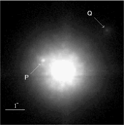
Figure 2: The non-coronographic image of HD 144987 with two new companions P and Q. The wings of PSF have the speckle structure. Primary component is saturated in a given intensity scale.

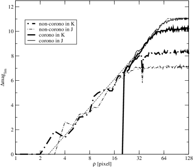
Figure 3: The detection curves for non-coronographic and coronographic images of HD 100546 in $J$ and $K$ bands. Coronographic curves start at $\rho\!=\!20$ pixels. The log-linear fit with a saturation plateau is used to approximate the combined curve in K (dashed line). The “spike” at $\rho\!=\!35$ pixels is caused by subtraction of the averaged PSF fitted by DAOPHOT (App. A).

Images with subtracted $P(\rho)$ were searched for point sources using the findobjs utility of Eclipse. The detection threshold was set to $3\sigma(\rho)$, where $\sigma(\rho)$ is the rms of azimuthal intensity fluctuations in the PSF wings at each $\rho$, also computed by jupe procedure. These thresholds were converted from pixel intensities to integrated fluxes with the help of Strehl ratios measured on non-coronographic images. Thus, limiting magnitude differences $\Delta J_{lim}(\rho)$ and $\Delta K_{lim}(\rho)$ were derived for each frame (see example in Fig 3).

The detection limits for the whole sample have some common characteristics. At small $\rho$, they are approximately proportional to $R=\log\rho$, with the average slope ${\rm d}K_{lim}/{\rm d}R=1.35\pm 0.22$. Further on, they saturate at some level which depends on the integration time. In coronographic images $K_{lim}$ saturates at about $K=16.8\pm 0.5$, about $2^{m}-3^{m}$ fainter than in non-coronographic images. It is possible to describe the detection limit by a merged curve which consists of the non-coronographic linear part for $\rho\!\leq\!1\arcsec$ and coronographic part for $\rho>1\arcsec$. This curve, typically, is continuous at the junction point $\rho\!=\!1\arcsec$ (Fig. 3). In other words, in the area close to the mask edge the residual speckle noise in a coronographic image with subtracted $P(\rho)$ and in the respective non-coronographic image with subtracted average PSF (App. A) is roughly the same. Individual log-linear slopes and saturation levels of the merged detection curves were found for each target star. They were subsequently converted into limiting mass ratios $q_{lim}(\rho)$ (Sec. 4.4).

3.3 Photometry of target stars

The majority of targets in our sample did not have any reliable measurements of near-IR magnitudes and colors before our study. To measure the flux, we must integrate the signal in an aperture as large as possible, reducing the dependence of the result on image quality. Efficiency of AO correction changed significantly as seeing varied from $0\aas@@fstack{\prime\prime}5$ to $2\aas@@fstack{\prime\prime}0$ during our run. Also, the result must be insensitive to detector imperfections and to the presence of other sources in the field of view. We computed the flux of the target star as

$$Flux=\sum\limits_{\rho<2\arcsec}I(x,y)+\int\limits_{2\arcsec}^{5\arcsec}{P(\rho)2\pi\rho{\rm d}\rho},$$ (1)

where the first term is the sum of pixel values $I(x,y)$ in a circle of $2\arcsec$ radius and the second term is an integral of the median radial profile. Median averaging effectively removes all distant ($\rho>2\arcsec$) sources and detector defects. For binary targets with $\rho<2\arcsec$ the flux of each component was then computed from the total flux and the magnitude difference as found by PSF fitting.

Integration of the median profile $P(\rho)$ gives a somewhat lower flux than direct integration of intensity, because average intensity of speckles is higher than their median intensity. Nevertheless, special tests have shown that this bias is less than 1% (or $0.01^{m}$) in all cases.

The magnitudes were reduced to zenith with average extinction coefficients of $0.08$ in $J$ and $0.10$ in $K$. The errors caused by extinction uncertainty are negligible because all objects were observed close to zenith. The photometric zero points were determined from the primary standard star HD 161743 and confirmed by 5 other stars for which $J$ and $K$ magnitudes were taken from Simbad. All determinations are mutually consistent to within $\pm 5\%$.

The resulting $K$ magnitudes and $J\!-\!K$ colors of primary components are given in Table 1. The errors reflect the deviations of individual fluxes from the mean and also take into account the flux difference between two halves of the data cubes (Sect. 3.1). Observations in non-photometric conditions are marked by “c” in the flags column. For these targets, measured $J$ and $K$ magnitudes represent only upper limits; the lowest of measured magnitudes was adopted.

We have computed the expected magnitudes $K_{\rm theo}$ based on the spectral types and visual magnitudes of all sample stars. These estimates agree well with the actual data for the majority of targets measured in photometric conditions: the difference $K_{\rm obs}-K_{\rm theo}$ shows a rms scatter of $0.^{m}15$ and its absolute value is less than $0.^{m}4$ for all targets but two.

These two outliers with $K$ excess of about $1^{m}$ are HD~100546 and HD~143275. The first star is reported to harbor a significant amount of circumstellar dust (Augereau et al. Augereau01 (2001), Meeus et al. Meeus01 (2001)) which is a natural origin of an increased infrared luminosity. The second star ($\delta$ Sco) was intensively studied and its photometry from Simbad ($K\!=\!2.75$) agrees much better with $K_{\rm theo}$ than our own measurement ($K\!=\!1.85$). Our result could possibly be explained by an error of ADONIS shutter timing at short (0.02 s) exposure. HD 143275 is a brightest star in our sample. Nevertheless, other bright stars were also observed with such integration time and an estimated random shutter error does not exceed 0.003 s.

On the other hand, $\delta$ Sco is a multiple star with Be-type primary and complex light variations. An extended study is published by Otero et al. (Otero01 (2001)) where the observations of a “$\gamma$ Cas-like outburst” are reported. The peak magnitude of $1.^{m}9$ in the visible was detected just two months after our observations. The authors explain this event as being caused by the periastron passage in a close multiple star. This is a second, more attractive astrophysical explanation of our discrepant photometry.

Based on a comparison of observed and expected $K$ magnitudes, we have extended the validity of companion’s photometry to 16 stars which were observed on non-photometric nights but for which $|K_{\rm obs}-K_{\rm theo}|<0.3$ and $J\!-\!K$ colors deviate from the estimated by less than 0.06. These cases are marked as “+” in the flags column of Table 1. The external errors of our photometry must be not larger than $\pm 0.^{m}1$ in $K$ and $\pm 0.^{m}15$ in $J\!-\!K$.

3.4 Photometry and astrometry of companions

The program findobjs provides approximate positions and brightness of detected sources. The final measurement of their relative coordinates and magnitudes was made with the profile-fitting utility NSTAR of DAOPHOT package (Stetson Stetson87 (1987)). Image of the primary star (if single) taken without coronograph was selected as PSF model for fitting distant ($\rho>1\aas@@fstack{\prime\prime}75$=35 pixels) components, whereas synthetic average PSFs (App. A) were used for closer pairs. Positions of primaries on coronographic images were inferred by indirect techniques with reduced accuracy (App. B). The characteristic error in position is 0$\aas@@fstack{\prime\prime}$005 – 0$\aas@@fstack{\prime\prime}$010.

Relative component positions in pixel coordinates were transformed into arcseconds. For calibration, we used binary stars HD 120709 and HD 199005 AB measured by Hipparcos. Pixel size was found to be $0\aas@@fstack{\prime\prime}0497\pm 0\aas@@fstack{\prime\prime}0005$, and the orientation of detector rows was found to be east-west to within $\pm 0\aas@@fstack{\circ}1$. Measurements of several additional known binaries confirmed this calibration.

The magnitudes and relative positions of 96 secondary components are given in Table 3.4 (its full version is published electronically).

Table 2: Photometry and differential astrometry of companion stars. Only data for observed non-optical components are shown here. Last column gives the status of companions (see text), new companions are marked; “?” in the Comp column denotes uncertain detections. Field flag contains “c” for data obtained in non-photometric conditions or “+” for likely photometric conditions (Sect. 3.3); “:” denotes incomplete resolution.

HD	Comp	K	$\epsilon_{\Delta K}$	$J$-$K$	$\epsilon_{\Delta(J\!-\!K)}$	flag	$\rho\arcsec$	$\epsilon_{\rho}\arcsec$	$\theta\degr$	$\epsilon_{\theta}\degr$	$N_{obs}$	Status
98718	B	5.86	0.01	-0.03	0.01		0.354	0.005	143.6	0.5	1	P
100841	P?	6.81	0.27			+	0.734	0.038	135.2	3.0	1	P new
104878	B	7.00	0.02	0.07	0.08	c	0.698	0.008	157.9	0.2	2	P
108250	P	10.50	0.03	1.01	0.05	+	2.362	0.024	53.2	0.1	1	P new
109668	P	10.94	0.26	0.82	0.29	c	4.853	0.049	198.3	0.1	3	P? new
113703	P	9.16	0.02	0.47	0.02	c	1.551	0.016	268.2	0.2	2	P new
116087	B	7.03	0.07	-0.11	0.23		0.164	0.010	135.2	3.6	2	P
120324	P	10.06	0.05	1.02	0.18	c	4.637	0.047	304.2	0.1	2	P new
120709	B	6.32		0.02			7.878	0.079	105.8	0.1	1	P
130807	B	6.84	0.01	-0.12	0.08	c:	0.099	0.008	86.0	7.3	1	P
131120	P	9.43	0.10	0.85	0.12		1.046	0.012	161.1	0.4	2	P new
132200	C	5.46	0.04	-0.04	0.04		0.128	0.008	156.4	1.9	1	P
132200	B	8.45	0.03	0.61	0.03		3.950	0.040	83.0	0.1	2	P
133937	P?	11.05	0.02			c	0.006	0.048	293.2	0.1	1	P new
136504	B	5.55	0.06	0.42	0.12	+	0.279	0.008	149.2	1.0	1	P
140008	B	9.47	0.05	0.42	0.05	c	0.507	0.009	132.8	0.8	1	P
142378	B	7.78	0.01	0.23	0.02		0.524	0.006	119.7	0.5	1	P
144217	B	6.80	0.05	-0.78	0.12	c	0.292	0.010	170.5	3.1	1	P
144218	E	7.43	0.05			c:	0.119	0.005	36.3	2.5	1	P
144987	P	9.75	0.08	0.57	0.12		1.119	0.015	116.9	0.3	5	P new
144987	Q	12.81	0.06	1.04	0.26		3.056	0.032	228.0	0.2	3	P? new
145502	B	5.14	0.01	0.06	0.01	+	1.334	0.014	1.8	0.1	1	P
145792	B	8.07	0.02	0.62	0.02		1.693	0.018	219.8	0.2	2	P
147165	C	4.77	0.07	0.06	0.07	+	0.469	0.006	244.4	0.4	1	P
151890	P	10.33		2.02		c	9.154	0.092	210.2	0.1	1	P? new
157056	B	5.02	0.24				0.300	0.025	251.6	3.3	1	P

The approximate (as given by findobjs) magnitudes of some one hundred field stars found in sky frames are provided in Table 3. These data are used to estimate the surface density of background stellar population. In both tables the $K$ magnitudes and $J\!-\!K$ colors are given with their errors. The errors are inferred from the scatter of individual values obtained from the measurement of different frames. Errors in Table 3.4 are those of magnitude differences and do not include uncertainties of primary star magnitudes. The cumulative distributions of $K$ magnitudes of sources around targets and in the sky frames are shown in Fig. 4. The majority of sources are faint, close to the detection limits at $K\approx 16^{m}$.

Figure 4: Cumulative distributions of $K$ magnitudes of all sources found in target frames (dotted line) and in sky frames (dashed line). The distribution of sources in target frames which are considered as optical (Sect. 4.2) is plotted in solid line which resembles the dashed curve of sky-frame background sources.

Few bright binaries from Table 3.4 were measured by Hipparcos or Tycho (ESA, Hipparcos (1997)) in the visible. The comparison of their magnitude differences in the $K$ band with $\Delta V_{T}$ or $\Delta Hp$ is shown in Fig. 5.

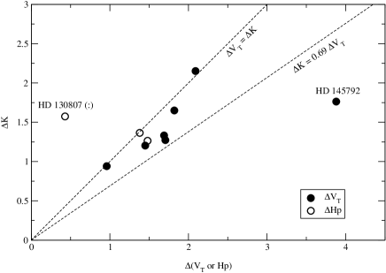
Figure 5: Comparison of the magnitude differences in the $K$ band with visual magnitude difference from Hipparcos ($\Delta Hp$) or Tycho ($\Delta V_{T}$, Fabricius & Makarov Fabricius00 (2000)). The leftmost point represents the closest ($\rho\approx 0\aas@@fstack{\prime\prime}1$), unreliably measured pair HD 130807; the rightmost HD 145792 is possibly an infrared companion. Two straight lines represent the equal differences (upper) and the ones expected from the standard relations (Lang Lang92 (1992)).

Four stars from our sample (HD 100841, 113902, 126981, 145483) were also observed by Hubrig et al. (Hubrig2001 (2001)). They did not detect the bright companion to HD 100841. The reality of this component is dubious; it is not seen in our $J$-band images either. On the other hand, an additional close (0$\aas@@fstack{\prime\prime}$2) companion to HD 145483 was found by Hubrig et al.; we did not observe this target because it has a known companion at $3\aas@@fstack{\prime\prime}8$. Another suspicious component is HD 133937 P, which is not seen in $J$ but quite prominent in our sole $K$-band image. This star and HD 100841 P need more observations to confirm their reality.

4 Statistics of companions

4.1 The color-magnitude diagram

In Fig. 6 the color-magnitude diagram is given. Only the stars observed under photometric conditions are plotted. Some red companions fall beyond the right boundary of the plot. The $J$ magnitude is taken as a photospheric luminosity indicator since it is known to be relatively free of IR excess, unlike $K$ magnitude.

Figure 6: The color-magnitude diagram. Filled circles – physical secondaries, empty circles – optical secondaries, crosses – primaries. Only the stars with valid photometry are plotted. Line is the Main Sequence for a distance modulus of 5.73, extending from B0V to M6V. The 3 Myr and 10 Myr isochrones for masses from 1.5 down to 0.08 solar mass are plotted as well (lines with triangles). Small asterisks – low-mass population of the Sco OB2 association from (Walter et al. Walter94 (1994)). A short segment shows the reddening vector for $A_{V}=1^{m}$.

The Main Sequence (MS) is traced from the data of Lang (Lang92 (1992)) for a fixed distance modulus of $5.^{m}73$ (140 pc). The primaries fall mostly near MS or scatter to the right from MS. The highly deviating point belongs to HD 100546 (Sect. 3.3). In general, the measured $J\!-\!K$ colors are validated by this plot.

The isochrones for 3 Myr and 10 Myr ages are based on the data of d’Antona & Mazzitelli (dAntona94 (1994), DM94) (for low-mass stars, we used their tracks computed with Alexander, Rodgers and Iglesias opacities and CM convection, shown to correspond to real PMS stars by a number of authors). Small triangles mark the masses of 1.5, 1.0, 0.7, 0.5, 0.3, 0.2, 0.1, 0.08 solar masses. The effective temperatures $T_{e}$ and bolometric luminosities were converted to the observed $(J,J-K)$ parameters. This transformation is not precise, involving some assumptions; the tracks themselves are not quite secure, too.

New tracks were published by a number of authors recently. Among them, the work of Baraffe et al. (Baraffe98 (1998)) is most useful, giving the synthetic absolute $J$ and $K$ magnitudes instead of $T_{e}$ and bolometric luminosities. Thus, the comparison with observations is more direct. We found that new isochrones do not differ from those of DM94 very significantly. Although the slim available data on PMS masses seem to support the Baraffe et al. tracks (Steffen et al. Steffen01 (2001)), the new tracks do not reproduce well the mass-luminosity (M-L) relation of older MS stars.

The actual colors and magnitudes of the low-mass PMS population in Sco OB2 are plotted in Fig. 6 by small asterisks using the data of Walter et al. (Walter94 (1994)). Those authors estimate that the masses of these X-ray selected stars range from 0.2 to 2 solar, the typical extinction is $A_{V}\approx 0.5$, and the age is around 1 Myr. We express some reservations about this age estimate, because OB stars are much older (de Zeeuw et al. deZeeuw99 (1999)).

4.2 Status of the secondary components

The secondaries known to be physical are either on MS or above. Some newly discovered components also fall within the low-mass zone and can be classified as physical. On the other hand, most of the faint secondaries are optical. The lower limit for physical secondaries corresponds roughly to $J=13$ or $K=12$ (for 3 Myr age). Some secondaries have $J-K>1.7$, falling outside the graph boundary. We presume that they are heavily reddened background stars.

All previously known components are considered here as physical. The reason for this is that the Sco OB2 association has a relatively large proper motion of 40 mas/yr, and any background component would show up by its fast motion relative to primary. This argument does not apply, however, to the association members that project close to the targets.

All new components fainter than $K=12$ or $J=13$ are considered as optical. The remaining bright opticals are identified on the color-magnitude diagram when valid photometry is available. Otherwise, an uncertain status is assigned. On the total, there are 37 physical components, of which 10 are new (3 of them have uncertain status and 1 is a questionable star HD 100841 P). The total number of new optical components is 70.

The status codes in Table 3.4 are:

P -

for physical companions;

P? -

for uncertain physical companions;

O -

for definitely optical (background) companions;

O? -

for likely optical companions.

The part of the Table 3.4 reproduced in this paper gives information on all observed non-optical companions. The discrimination between the optical and physical secondaries is one of the important issues in this study and potentially a weak point. Naturally, all new components have small masses and their classification directly affects the lower bin of the mass ratio distribution. In Sect. 4.5 we consider the 3 uncertain companions as physical. Our guess is that 1 or 2 of them may be optical, but this revision would only reinforce our main conclusions.

4.3 Statistics of background sources

Figure 7: Distribution of the density of background (optical) components in the sky. The fields with no opticals are plotted as empty squares. The $+$ crosses indicate optical components in the main fields, x crosses – in the sky fields, with cross size proportional to the number of components.

In Fig. 4 the cumulative distribution of the optical components (number of components $N$ that are brighter than given magnitude) is plotted in full line. Only components with $\rho>3\arcsec$ were selected (at smaller separations, the companion detection in the coronographic frames is affected by the halo of the primary). Dashed line shows the same distribution for the sky fields. Only companions detected in both $J$ and $K$ bands were selected.

The two curves coincide to within statistical fluctuations, especially in the important region around $K=12-14$ where the discrimination between optical and physical components is critical for our analysis. We note that the total surface of main fields is smaller than the surface of sky fields by 15% (central $3^{\prime\prime}$ excluded). On the other hand, the detection limits in the sky fields may be lower because of the lower Strehl ratio (anisoplanatism). All in all, there are 5 components brighter than $K=12$ in the sky fields and 3 such optical components in the main fields. Taken at face value, it means that about 2 components in the main fields may be still mis-classified as physical. However, it is clear that our classification scheme did not miss a large number of faint physical companions, otherwise we would observe an excess of “opticals” in comparison with the sky fields.

An important feature of background sources is their highly fluctuating density (Fig. 7). For 45 targets, no optical components were found neither in the main nor in the sky fields; on the other hand, in the remaining fields a significant correlation between the number of optical components in the main and sky fields was found. In 3 main fields, as much as 7 to 9 optical components were detected, with no less than 6 components in the corresponding sky fields. This correlation is a strong argument for the optical nature of faint components.

Quite often more than one component identified as optical are present in the main fields and have comparable separations. They can not be physical for yet another reason: non-hierarchical stellar systems are dynamically unstable and must disintegrate, given the age of Sco OB2 group.

In following sub-sections we consider the calculation of the mass ratios $q=M_{2}/M_{1}$. It will allow us to derive the mass ratio distribution $f(q)$ of physical systems.

4.4 Estimation of masses and mass ratios

In principle, masses of MS stars can be estimated from their $J-K$ colors. However, the colors are measured with large errors and are distorted by extinction and IR excess. Hence, the best way to estimate masses of the companions is to use their luminosities, preferably in the $J$ band. On the other hand, the use of mass-luminosity (M-L) relation requires a knowledge of distance and age (for low-mass stars), it relies also on the yet uncertain PMS tracks.

The M-L relations for MS and PMS stars are taken from Lang (Lang92 (1992)) and Baraffe et al. (Baraffe98 (1998)), respectively. For PMS tracks, the mass $M$ depends on $A$ (the logarithm of age in Myr) and absolute $J_{0}$ or $K_{0}$ magnitudes approximately as

$$\log(M/M_{\odot})\approx 0.706-0.305J_{0}+0.545A,$$ (2)

$$\log(M/M_{\odot})\approx 0.440-0.313K_{0}+0.581A.$$ (3)

For MS stars, the M-L relation was approximated by several linear segments. The accuracy of all these approximations is better than $\pm 10\%$ in mass. Of course, the actual isochrones are not linear but rather “saturate” as the luminosity reaches its MS value. So, the companion masses were calculated from both MS and PMS relations and the lowest of the two values was taken. The actual ages of subgroups were used in the calculations: 4.5 Myr for Upper Scorpius, 14.5 Myr for Upper Centaurus-Lupus and 11.5 Myr for Lower Centaurus-Crux (de Zeeuw et al. deZeeuw99 (1999)).

The M-L relation is favorable for mass estimation: its slope at MS roughly corresponds to $M\propto L^{0.5}$ and steepens to $M\propto L^{0.8}$ for the PMS tracks. This explains why the mass estimates are relatively insensitive to data reduction details.

The masses of primary stars were also estimated from their luminosities rather than from their spectral classes. This was done to cancel as much as possible the influences of errors in distances, extinction, etc., which affect the masses of primaries and secondaries in almost the same way and hence have little effect on the mass ratios $q$. Even the errors in the photometry caused by non-photometric conditions are compensated to some extent because $q$ depends mostly on the magnitude difference.

The detection limits were studied and modeled in Sect. 3.2. We convert the derived log-linear relations between $K_{lim}$ and $R=\log(\rho/1\arcsec)$ into the limiting mass ratio $q_{\rm lim}$ using the M-L-Age relation in the $K$ band and the actual age of each target. $K$-band is used since low-mass red companions are better detected at longer wavelengths. These limiting mass ratios are sorted in increasing order and plotted in Fig. 8 as detection probability (bias). If all frames were taken in exactly the same conditions, all $q_{\rm lim}$ would be identical. The actual distribution of $q_{\rm lim}$ reflects the spread in the observing conditions, exposure time, target brightness, etc.

Figure 8: The fraction of detectable components as a function of mass ratio $q$ for separations from $0\aas@@fstack{\prime\prime}2$ to $0\aas@@fstack{\prime\prime}9$, as indicated by numbers near the curves.

The detection bias is modeled as a set of linear functions of $\log q$, neglecting the “tails” of the distributions in Fig. 8. Linear models are defined by two parameters, the $\log q_{lim}$ where 50% of companions are detected and the full range in $\log q_{lim}$. These parameters were represented by quadratic functions of $R$. The analytical model of detection bias is plotted in Fig. 9.

4.5 Mass ratio distribution and companion fraction

The distribution of the physical secondaries in the $(\log\rho,q)$ plane is shown in Fig. 9. It is expected that the component distribution in $\log\rho$ should be uniform (Öpik’s law). Indeed, it seems to be the case. Moreover, there seems to be no significant correlation between $\rho$ and $q$ in the separation range studied. This permits to discuss the $q$ distribution for all relevant separations jointly.

Figure 9: The distribution of the known and measured (squares), known and unmeasured (pluses) and newly discovered (asterisks) physical components in the $(\log\rho,q)$ plane. The detection model is shown by solid line (50% detection) and dashed lines (0% and 100% detection). The separation range selected for statistical analysis is delimited by the vertical lines.

Figure 10: Left: The histogram of the mass ratio distribution $f(q)$ in separation range from 45 to 900 A.U. (full line). Dashed line shows the uncorrected value in the first bin. Asterisks – re-normalized $f(q)$ of G-type dwarfs with periods $P\!>\!30$ yr ($a>10$ A.U.) from DM91. Dotted line corresponds to $f(q)\propto q^{-0.5}$, dash-dot – to $f(q)\propto q^{-1.8}$. Right: cumulative distribution corrected for detection incompleteness (crosses) and its modeling as $F(q)=q^{0.5}$.

We limit the statistical analysis to the separation range from $0\aas@@fstack{\prime\prime}3$ to $6\aas@@fstack{\prime\prime}4$, which corresponds to 45–900 A.U. at the distance of Sco OB2. For lower separations, the detection bias in $q$ becomes too important. The upper limit is determined by the half-size of the frames. Components at larger separations were actually detected in the corners, but, as evident from Fig. 9, little can be gained by extending the limit to $9\arcsec$ and making corrections for incomplete surface coverage.

A total of 27 physical components fall in the selected separation range which covers 1.3 decades. Assuming that the distribution in $\log\rho$ is uniform and that the distribution in $q$ is smooth, we estimate the fraction of missed components by integrating the bias model within the selected limits for each bin of the $q$ histogram. The fraction of detected components is more than 0.8 for all bins, which means that our incompleteness correction remains reasonably small. The resulting histogram of $q$ (after correction for incompleteness) is plotted in Fig. 10 (left).

The same data reduction steps were done for the DM94 tracks and two fixed ages of 3 and 10 Myr. The results are qualitatively very similar. Comparing the histograms for these two isochrones, we saw that assuming a younger age results in lower masses, slightly re-distributing the components between the two lowest bins.

In Fig. 10 (right) the same histogram is plotted as cumulative distribution, in order to avoid binning. It is corrected for detection incompleteness by increasing the “weights” of low-$q$ systems accordingly. The slope of the cumulative distribution clearly increases towards low $q$. Adopting the power law $f(q)\propto q^{-\Gamma}$, it seems that the index $\Gamma\!=\!0.5$ fits well the data.

The $q$-distribution does grow towards low $q$, but only mildly. On the other hand, the power law with index $\Gamma$ from 1.8 to 2.1 is clearly rejected. Such power law corresponds to the initial mass function (IMF) in Sco OB2 (Brown Brown98 (1998), Preibisch & Zinnecker Preibisch99 (1999), Preibisch et al. Preibisch01 (2001)) and would apply if the secondary components were selected randomly from IMF.

The power-law distributions $f(q)\propto q^{-\Gamma}$ are not integrable for $\Gamma>1$, in this case the total binarity is determined by the elusive cut-off at low $q$. On the contrary, the actual distribution is smooth and integrable, the total binarity is well defined. The total number of components (after correction for incompleteness) is 29.6 for the 115 targets studied and in the separation range of 1.3 dex. This leads to a companion star fraction (CSF) of $0.20\pm 0.04$ per decade of separation or $0.13\pm 0.02$ per decade of period.

We repeated the analysis while excluding the 3 faint components with uncertain physical status and the 2 components with unsecure detection. The number of companions in the $0\aas@@fstack{\prime\prime}3-6\arcsec$ separation range becomes 23 (24.85 after correction for incompleteness), the CSF is revised down to $0.17\pm 0.04$. The lowest bin in the histogram (Fig.. 10 left) becomes 30% less, leading to even more uniform $f(q)$ which may be approximated by a $q^{-0.3}$ law. This exercise shows that our conclusions do not critically depend on the remaining uncertainties in the experimental data.

5 Discussion

Before our study, we suspected that the number of unknown low-mass visual components around B-type stars is large, because low-mass stars are, generally, much more frequent than high-mass stars, and because the detection of such components by traditional techniques was difficult. Now we see that the newly detected low-mass physical components are not so numerous and that the old detections were essentially complete down to at least $q=0.3$. It was indeed necessary to go much deeper in magnitude difference to validate the historical data! In this perspective, the fact that most of our newly detected components are optical is not disappointing.

Our result is in marked disagreement with the conclusions of Abt et al. (Abt90 (1990)) who claim that the distributions of the secondary components to B2-B5 stars follows the Salpeter mass function and increases steeply towards small $q$ in the range of separations studied here. Their analysis is based on the known visual components confirmed by common proper motions. Still, we strongly suspect that most of wide pairs in the B2-B5 sample of Abt et al. are optical. In their Table 5 there are 7 trapezium-type systems with separations in the $10^{\prime\prime}$ to $63^{\prime\prime}$ range and separation ratio less than 3 which are likely unstable, if physical. When the spectra of the components of 116 trapezium-type systems were taken by Abt & Corbally (Abt00 (2000)), they discovered that only 28 of them can be physical – a proof that most of the cataloged trapezia are indeed spurious.

Figure 11: Mass ratio as function of separation for the 56 low-mass PMS binaries in Sco OB2 studied by Köhler et al. (Kohler00 (2000)). The curve shows indicative detection bias, vertical lines indicate the separation range of their statistical analysis.

Table 4: Companion star fraction (number of companions per decade in separation) in different populations.

Spectral type,	$N$	Range,	CSF	Ref.
environment		A.U.
B, Sco OB2	115	45-900	0.20 $\pm$ 0.04	1
PMS, Sco OB2	118	20-900	0.21 $\pm$ 0.04	2
PMS, Sco-Lup	269	120-1800	0.12 $\pm$ 0.02	3
PMS, Tau-Aur	104	120-1800	0.22 $\pm$ 0.04	3
G, field	164	40-900	0.12 $\pm$ 0.03	4
M, field	58	10-1000	0.11 $\pm$ 0.04	5
A-K, Hyades	167	5-50	$>$0.16 $\pm$ 0.03	6
G-K, Pleiades	144	12-1000	0.14 $\pm$ 0.02	7
G-K, Praesepe	149	15-600	0.15 $\pm$ 0.03	8

References: 1 - this work; 2 - Köhler et al. (Kohler00 (2000)); 3 - Brandner et al. (Brandner96 (1996)); 4 - Duquennoy & Mayor (DM91 (1991)); 5 - Fisher & Marcy (Fischer92 (1992)); 6 - Patience et al. (Patience98 (1998)); 7 - Bouvier et al. (Bouvier97 (1997)); 8 - Bouvier et al. (Bouvier01 (2001)).

In Table 4 we give a summary of statistical binarity studies in different populations, to be compared to our results. The sample size $N$ and the approximate range of separations surveyed are indicated. The CSF (fraction of all companions per unit interval in the logarithm of separation) is only a weak function of separation, hence it is legitimate to compare results in different separation ranges. For the Hyades, the CSF given by Patience et al. (Patience98 (1998)) involved a factor of 2 correction for undetected systems, hence we preferred the uncorrected lower limit.

The most recent study of the multiplicity of low-mass population of Sco OB2 (Köhler et al. Kohler00 (2000)) is very similar to the present work by the number of targets surveyed and the separation range ($0\aas@@fstack{\prime\prime}13-6\arcsec$). They find a CSF of $0.21\pm 0.04$ per decade of separation, indistinguishable from our result. We tried to process the magnitudes and flux ratios of the 56 systems from their Tables 2 and 3 in the same manner as our data, converting the $K$ magnitudes into mass ratios with the help of a 3 Myr isochrone and for the assumed distance of 140 pc. The results are shown in Fig. 11. The curve indicates our best guess of the detection threshold, which is $\sim 3$ times higher than the threshold given by the authors themselves. About 7.8 systems in their sample (mostly with large separations) were estimated to be optical. Taking into account these uncertainties, it does not make sense to compare the histograms of $q$. All that can be said is that the $q$ distribution seems to be uniform and certainly does not increase towards small $q$ as much as would be expected from the IMF slope.

Brandner et al. (Brandner96 (1996)) provided a comprehensive summary of the previous binarity studies among the PMS stars which were made in the visible. The CSF in the Upper Scorpius and Lupus is $0.12\pm 0.02$ per decade of separation for a combined sample of 269 stars. The global CSF among 525 PMS stars is $0.14\pm 0.013$, which remains the most statistically sound estimate to date (however, in the Taurus-Auriga region the CSF is $0.22\pm 0.04$). Clearly, Köhler et al. obtained a significantly higher CSF for the same population. However, Brandner et al. find an evidence for CSF variations across the Sco OB2, and the regions studied by Köhler et al. happen to be near the binary-rich zone. This seems to be the most plausible explanation of this discrepancy.

Our sample covers a large region in the sky. For this reason the CSF=0.12 measured by Brandner et al. is more appropriate for comparison with our result, CSF=0.20. Thus, more massive B-type stars do have an an increased CSF with respect to the lower-mass PMS stars. The same conclusion is reached by comparing our result to the binary fraction of low-mass field dwarfs and low-mass cluster population (Table 4).

The unbiased mass ratio distribution for visual binaries with B-type primaries is the main result of this study. The idea of independent selection of the visual components from some initial mass function can now be definitely rejected. However, the new result is not so unexpected, after all. The $f(q)$ obtained by DM91 for the wide ($\log P({\rm days})>4$) systems is similar to the $f(q)$ found here (Fig. 10). The mass ratio should be indeed biased towards a uniform one by stellar dynamics, whatever the IMF. N-body simulations demonstrated that the shape of $f(q)$ depends on the density and composition of the stellar aggregate where the binaries have been formed, and a certain choice of parameters may reproduce the result of DM91 (Kroupa Kroupa95 (1995), Durisen et al. Durisen01 (2001)).

On the other hand, the secondary components of B-type stars must have been formed in the same clouds as their primaries, in conditions that likely favored high masses. The secondaries may thus be distinct from the rest of low-mass population in Sco OB2 with respect to their initial mass function and age. For the moment we are not able to disentangle the influence of dynamical and birth factors on the final mass ratio distribution. The important thing is that the distribution itself is now known with some confidence.

Appendix A Detection and measurement of close companions with DAOPHOT

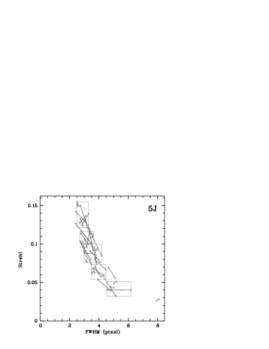
Figure 12: Example of the classification of images into groups by Strehl ratio (SR), used to produce average PSFs. The SR of images of the last (fifth) night in $J$ band are plotted against their Full Width at Half Maximum (FWHM); boxes denote the borders of groups. Lines connect the points which belong to two planes of the same data cube and reflect the fast variability of image quality.

In this appendix we present the solution of the problem of PSF selection for DAOPHOT fitting in non-coronographic mode. A simple subtraction of the radial profile of PSF (jupe algorithm) leaves the bright semi-static speckle pattern around the target star unattenuated. To remove it partially, we produced the set of average PSFs for each night and each filter, grouped by the value of the Strehl ratio (i.e. relative sharpness) of the image (Fig. 12). Being averaged over images of many objects, these synthetic PSFs contain no trace of any possible faint companions which hide under the speckle pattern (extra PSF cleaning function of DAOPHOT II removes all outlying features like median filtering). The radius of these synthetic PSFs is 35 pixels $=1\aas@@fstack{\prime\prime}75$ (maximal available in DAOPHOT from the used release of ESO-MIDAS).

All non-coronographic images of target stars were fitted with one of those average PSFs selected according to their own Strehl ratio. The residuals after PSF suntraction were visually searched for new close companions. The companions of all new and known close ($\rho<1\aas@@fstack{\prime\prime}75$) visual systems were simultaneously fitted with this method using NSTAR or ALLSTAR utility of DAOPHOT to produce the differential astrometric and photometric measurements reported in this paper.

To get an estimate of the detection limits achieved with subtraction of synthetic PSFs, we used again the jupe program. After subtraction, the intensity of the remaining speckle noise decreased to a level which, by chance, coincided with the detection limit in coronographic images (Fig. 3).

Appendix B Differential astrometry with coronograph

The coordinate differences between the source and target stars were measured in three different ways. The first and most reliable method is the simultaneous PSF fitting to primary and secondary stars in non-coronographic images.

However, simultaneous PSF fitting is not applicable to coronographic images since the primary star is not visible. Instead, the position of the primary was determined from the PSF wings by the jupe program. The relation between this method and direct PSF fitting was studied. The precision of jupe coordinates of a primary was found to be $\pm 0.3$ pixels, with a constant bias of $-1.5$ and $-0.6$ pixels in $x$ and $y$ directions, respectively. This bias is caused, possibly, by the asymmetry of the PSF wings.

Alternatively, the known positions of the primary in the two quadrants of non-coronographic images can be used to predict the position of the star under the mask, supposing that AO system stabilizes the image in the detector plane and that the offsets provided by the chopping mirror of ADONIS are precise and repeatable. These offsets were studied and calibrated. It turned out that the chopping mechanism moves the target star across the detector with an rms error of about $\pm 0.25$ pixels; the error never exceeds 0.6 pixels.

Whenever components were measured by several methods, resulting coordinates were computed as weighted averages, with weight 10 for direct PSF fitting, weight 1.5 for jupe coordinates and weight 2.0 for coordinates extrapolated from non-coronographic images.