Column Density Probability Distribution Functions in Turbulent Molecular Clouds: A Comparison between Theory and Observations.

Abstract

The one-point statistics of column density distributions of turbulent molecular cloud models are investigated and compared with observations. In agreement with the observations, the number N of pixels with surface density $\Sigma$ is distributed exponentially $N(\Sigma)\sim\exp(-\Sigma/\Sigma_{0})$ in models of driven compressible supersonic turbulence. However, in contrast to the observations, the exponential slope defined by $\Sigma_{0}$ is not universal but instead depends strongly on the adopted rms Mach number and on the smoothing of the data cube. We demonstrate that this problem can be solved if one restricts the analysis of the surface density distribution to subregions with sizes equal to the correlation length of the flow which turns out to be given by the driving scale. In this case, the column density distributions are universal with a slope that is in excellent agreement with the observations and independent of the Mach number or smoothing. The observed molecular clouds therefore are coherent structures with sizes of order their correlation lengths. Turbulence inside these clouds must be driven on the largest scales, if at all. Numerical models of turbulent molecular clouds have to be restricted to cubes with sizes similar to the correlation lengthscale in order to be compared with observations. Our results imply that turbulence is generated on scales that are much larger that the Jeans length. In this case, gravitational collapse cannot be suppressed and star formation should start in molecular clouds within a dynamical timescale after their formation.

1 Introduction

High-resolution observations in many wavelength regimes have revealed the complex structure of molecular clouds. This cold gas component of the interstellar medium is characterized by irregular, clumpy and filamentary substructures (e.g. Blitz 1993; Williams, Blitz & McKee 2000), the origin of which is not well understood up to now (Burkert & Lin 2000). Observed linewidths are much greater than thermal, suggesting supersonic random motions with thermal Mach numbers that reach 50 on large scales. Compressible turbulence and magnetic fields are likely to play an important role in regulating the dynamical evolution and star formation history in molecular clouds (Shu, Adams & Lizano 1987; McKee et al. 1993; McKee 1999; Klessen & Burkert 2000, 2001; Klessen, Heitsch & Mac Low 2000; Padoan & Nordlund 1999; Heitsch, Mac Low & Klessen 2001; Burkert 2001).

Due to its complexity, molecular cloud turbulence has been investigated primarily numerically. Recent progress in this field is reviewed by Vázquez-Semadeni et al (2000). The simulations show that driven and decaying turbulence leads to density distributions that resemble the observed structures (e.g. Passot, Vázquez-Semadeni & Pouquet 1995; Balsara et al. 1999; Padoan & Nordlund 1999; Ostriker, Gammie & Stone 1999, 2001; Klessen 2000; Mac Low & Ossenkopf 2000). In addition, the models demonstrate that the supersonic motion decays surprisingly fast, on timescales of order or less than the dynamical timescale, even in those cases where the magnetic field is dominant (Mac Low et al. 1998; Stone, Ostriker & Gammie 1998; Mac Low 1999; Smith, Mac Low & Heitsch 2000). Either molecular clouds are not dynamically supported but instead represent transient cold structures in the state of gravitational contraction and star formation (Ballesteros-Paredes, Hartmann, & Vázquez-Semadeni 1999; Elmegreen 2000; Pringle, Allen & Lubow 2000; Hartmann, Ballesteros-Paredes & Bergin 2001) or there exists a yet unknown driver of turbulence (Heitsch, Mac Low & Klessen 2001), such as field supernovae (Mac Low et al. 2001).

It is however not clear whether current numerical models provide a suitable description of the dynamical state of molecular clouds. Several simplifying assumptions are being made that could affect the results. For example, periodic boundary conditions are often adopted. The turbulent state is typically generated by setting up a Gaussian random velocity field and an initially homogeneous density distribution. The number of grid cells and thus the spatial resolution is very limited. In order to test the validity of numerical models it is therefore crucial to compare quantitatively the density structure generated by the simulations with the observations. Fortunately, despite their irregularity, molecular clouds reveal some interesting global properties. One example are the Larson relations (Larson 1981) which couple the structural and dynamical properties of cloud clumps, defined as high-density regions of coherent motion, although the mean density-size relation has been called into question (Ballesteros-Paredes, Vázquez-Semadeni, & Scalo 1999, Ballesteros-Paredes & Mac Low 2001).

Another robust observable which can be compared easily with theoretical models is the one-point statistics of cloud column density distributions. This quantity has been studied by Blitz & Williams (1997, 1999) and Williams et al. (2000). They used two-dimensional column density maps of clouds observed in different radial velocity bins for an optically thin molecular species. For each pixel of this three-dimensional data cube, characterized by galactic latitude, longitude and radial velocity, the antenna temperature was determined, which correlates with the column density of the gas moving with the corresponding radial velocity. The column density probability distribution function (PDF) was then defined as the total number $N$ of pixels with a certain column density $\Sigma/\Sigma_{max}$. Here $\Sigma_{max}$ is the maximum column density found in the data cube. Blitz & Williams (1997, 1999) showed that for a linear binning of the column density, the PDFs of molecular clouds follow a universal exponential profile in the regime 0.2 $\leq\Sigma/\Sigma_{max}\leq$ 1 that can be well approximated by the empirical formula

$$\log(N/N_{0.3})=\frac{0.3-\Sigma/\Sigma_{max}}{0.35}$$ (1)

where $N_{0.3}$ denotes the number of pixels with $\Sigma/\Sigma_{max}=0.3$. In addition, they found a relative lack of high-density pixels for very high-resolution observations with pixel sizes smaller than 0.25–0.5 pc. This scale corresponds to length scales where the velocity dispersion of the turbulent gas is of order the thermal sound speed and where coherent molecular cores appear that are the sites of star formation. Observations of column density PDFs have also been analyzed, in different ways, by Miesch & Bally (1994) and compared to simulations by Klessen (2000).

The universal PDF predictions of Blitz & Williams can be easily compared with numerical simulations. They are therefore ideally suited to test theoretical models of molecular cloud structure and evolution. A Gaussian distribution would for example be expected if the density distribution were random. The distribution will however be different for turbulent flows with large coherent structures like shock fronts. Ostriker, Stone & Gammie (2001) did show that their turbulent cloud models lead to log-normal, rather than Gaussian distributions of column densities with a weak dependence on the magnetic field. Vázquez-Semadeni & García (2001) showed that column density PDFs have exponential tails if the line of sight does not pass through many correlation lengths. They however restricted their simulations to mildly supersonic turbulence with rms Mach numbers of order 2 and did not subdivide their simulated data cubes into velocity bins. No simulation has up to now been compared quantitatively with the results of Blitz & Williams (1997, 1999).

In this paper we investigate the column density PDFs that result from MHD simulations of driven, turbulent, molecular clouds. The numerical models are summarized in section 2. In section 3 we show that the PDFs of these models have exponential high-density tails, as observed. A comparison with the observations unveils two problems, however. First, the exponential slope which corresponds to the typical over-density is not universal but depends strongly on the adopted Mach number. Even for very high Mach numbers the exponential slopes of the simulated data cubes are too steep compared with the observations. Secondly, in contrast to the observations, smoothing does not lead to saturation. We demonstrate that these problems can be solved if one restricts the analysis to regions with sizes of order the correlation lengthscale of the turbulent medium. Section 4 summarizes the results.

2 The numerical model

In the following sections we will analyse a set of three-dimensional numerical simulations of driven, isothermal, hypersonic turbulence with and without magnetic fields, described in more detail by Mac Low (1999). These computations were performed with ZEUS-3D, a second-order, Eulerian, astrophysical MHD code (Stone & Norman 1992; Clarke 1994) using Van Leer (1977) advection. Shocks are resolved using a Von Neumann type artificial viscosity.

The computations were performed on a Cartesian grid with uniform initial density and periodic boundary conditions in every direction, to simulate a region within a molecular cloud. The turbulence is driven in order to maintain a state of roughly constant turbulent Mach number (defined as the ratio between rms gas velocity and isothermal sound speed) despite energy dissipation at the grid scale and in shocks. The driver consists of a field of Gaussian perturbations applied to the model velocities with flat spectrum extending over a narrow range of wavenumbers given by $n-1<|\vec{k}|<n$ for models named HX$n$ (see table 1 in Mac Low 1999). The normalization of the perturbations is adjusted at each timestep to maintain a constant energy input rate, as designated by the second letter in the model names (with A being the lowest rate, and E being a factor of 100 higher, with the letters indicating half dex steps). The resulting models have density contrasts of two to six orders of magnitude, depending on the strength of the driving. Images of these models are shown in Fig. 4 of Mac Low (1999).

3 The distribution of column densities of turbulent cloud models

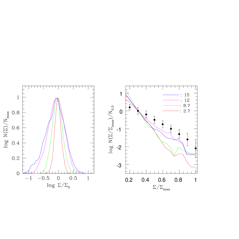
A detailed investigation of the column density PDFs of the numerical models shows that the distribution of column densities is not sensitive to the adopted magnetic field or the driving wavelength in the region $\Sigma/\Sigma_{max}\geq 0.2$. The shape of the PDFs does however depend strongly on the Mach number of the turbulent flow. As an example, Figure 1 shows the PDFs of four different simulations that correspond to turbulent Mach numbers of 2.7, 8.7, 12 and 15, respectively (models HB8, HE8, HE4 and HE2, defined in table 1 of Mac Low 1999). The left panel of Fig. 1 shows a log-log representation of the PDFs of the models. In order to compare the results with previous work, a logarithmical binning was adopted with no subdivision into velocity bins. In agreement with the study of decaying supersonic turbulence by Ostriker, Stone & Gammie (2001) we find that the distribution is log-normal with roughly equal numbers of over-dense and under-dense regions and a width that increases with increasing Mach number.

The right panel shows the normalized PDFs if the column density is binned linearly. Here we adopt 8 velocity bins that are equally spaced in the range defined by the projected minimum and maximum velocity. Varying the number of velocity bins between 4 and 16 does not change the profiles significantly. The distribution of overdense regions can be approximated well by an exponential with a slope that depends strongly on the Mach number. Compared with the observations of Blitz & Williams (1997, 2000), the low Mach number cases can clearly be ruled out. Although the profiles become flatter with increasing Mach numbers even the M=15 case is still steeper than observed.

Blitz & Williams (1997, 1999) examined the column density PDFs of the Taurus molecular cloud with exceptionally high resolution using the data of Mizuno et al. (1995). At high resolution they found a steepening of the profile at the high column density end ($\Sigma/\Sigma_{max}>0.7$). They found that this feature disappears and that the PDF becomes exponential again with the same slope as in other cloud regions if the resolution was degraded by an order of magnitude. Further smoothing did not change the slope. They interpreted this effect as a signature of self-similarity on large scales and a break in self-similarity on a with an additional high column density component becoming visible at spatial resolutions of 0.1 pc. In order to test the effect of smoothing, the solid line in Fig 2 shows the PDF of model HC8, a numerical simulation with $256^{3}$ grid cells, a Mach number M=4 and driving on a scale of 1/8 th the box size. The exponential slope of this very high-resolution simulation is again much steeper than observed and in agreement with low-resolution M=4 test cases. We smoothed the PDF by averaging the surface density distribution over regions of $n\times n$ grid cells, where n is the smoothing factor. Figure 2 demonstrates that the PDFs become flatter with increasing smoothing factor. With smoothing by a factor of 8 (long dashed line), the PDF is in agreement with the observations. It however flattens further when we increase the smoothing factor to $n=16$. In contrast to the observations, smoothing of the whole cube does not saturate.

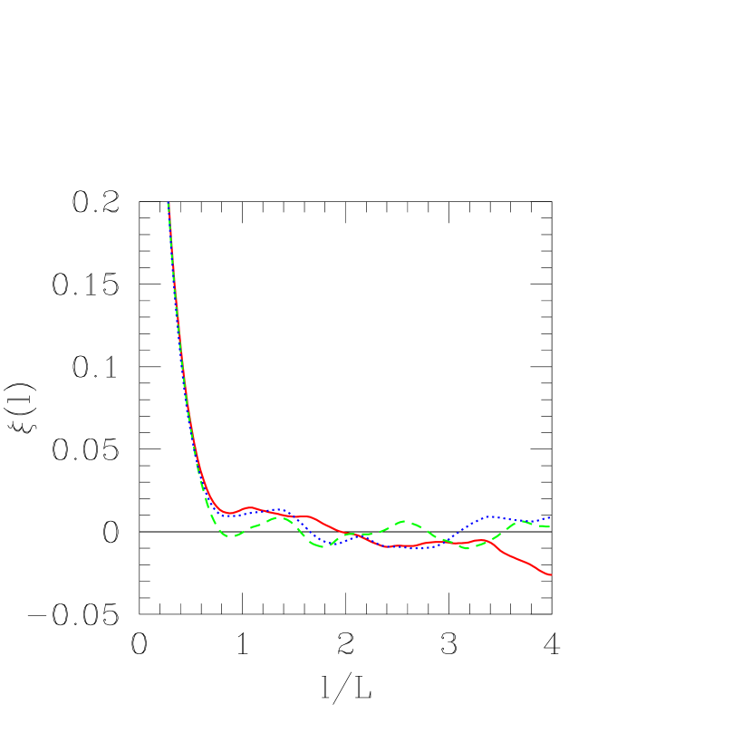
Vázquez-Semadeni & García (2001) found that the shape of the column density PDFs depends on how many correlation lengths their lines of sight passed through. We measured the autocorrelation spectra of our turbulent boxes. As an example Figure 3 shows the normalized autocorrelation function

$$\xi(l)=\frac{\langle\rho(\vec{r})\times\rho(\vec{r}+l\vec{e}_{x,y,z})\rangle}{\langle\rho(\vec{r})\times\rho(\vec{r})\rangle}$$ (2)

of model HC8 as function of $l/L$. $\vec{e}_{x,y,z}$ are the unit vectors in the x,y and z direction, respectively, of the numerical grid. L denotes the driving lengthscale which for model HC8 is 1/8 th of the box size. As expected for non-magnetic, isotropic turbulence, $\xi$ is independent of the direction. It decreases fast with increasing separation and becomes zero for $l>L$. We find in all cases that the correlation length is equal to the driving scale of the turbulence, with virtually no dependence on the rms Mach number or magnetic field strength. Regions with sizes smaller than the driving scale are correlated, larger regions are uncorrelated.

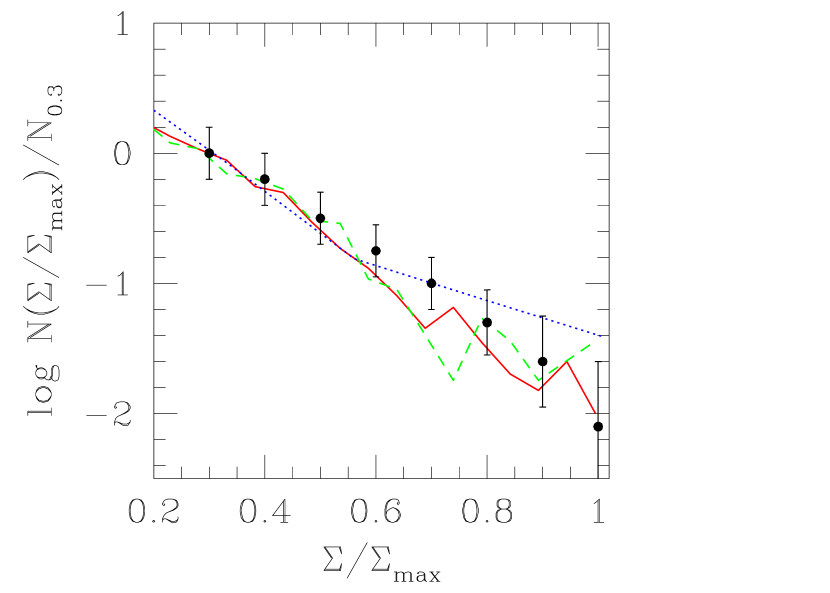
Each of our turbulent boxes contains five to ten correlation lengths. The question now arises whether the previous results change if one analyses only regions that are strongly correlated. We therefore examined the properties of the turbulent flow in a subregion of the full model with box length equal to one correlation length. Figure 4 shows the resulting normalized column density PDFs for model HC8. The distribution is exponential, but now new properties emerge. The PDF is in very good agreement with the observations although the Mach number is quite small (M=4). In addition, the exponential slope now no longer depends on smoothing. An investigation of the other models confirms this result. Restricting the analysis to regions with one correlation length, the PDFs agree well with the results of Blitz & Williams (1997, 1999), both qualitatively and quantitatively, and independent of Mach number or smoothing as long as the turbulence is supersonic.

4 Discussion

Our comparison of turbulent models to the observations analyzed by Blitz & Williams (1997, 1999) indicates that real molecular clouds are objects containing only one correlation length. We find that in driven turbulence models this correlation length lies within factors of order unity of the adopted driving scale of the turbulence. This suggests that molecular clouds are driven on the largest scales, comparable to their sizes, if at all. A similar conclusion was reached by Mac Low & Ossenkopf (2000) based on the self-similarity seen at all scales below the largest scales in wavelet transform spectra of the clouds. One large-scale mechanism could be field supernovae from previous star formation episodes within the nearest several hundred pc (Norman & Ferrara 1996, Mac Low et al. 2001).

Klessen, Heitsch & Mac Low (2000) and Heitsch, Mac Low & Klessen (2001) demonstrated that star formation inside molecular clouds could only be completely suppressed by turbulent flows if the driving scale is smaller than the local Jeans length, which is small compared to the cloud size. Our results imply that turbulence is generated on scales which are similar to the cloud size. Turbulence therefore cannot prevent gravitational collapse on smaller scales. This is consistent with the observation of at least low-mass star formation in virtually every observed molecular cloud.

Figure 1: The PDFs of four models of driven turbulence are shown with logarithmic (left panel) and linear binning (right panel). The equilibrium Mach numbers of the curves are indicated in the upper right corner of the right panel. Points in the right panel show the observed distribution with errorbars indicating the observed variations in the PDFs of different cloud regions.

Figure 2: Surface density PDFs of a high-resolution model with M=4. The solid line shows the unsmoothed PDF, adopting 8 velocity bins. The other lines show the effect of smoothing by a factor of 2,4,8 and 16. The PDFs become flatter with increasing smoothing factor. Points with errorbars indicate the observational range.

Figure 3: The three curves show the autocorrelation function $\xi(l)$ of model HC8 in the x,y and z direction of the numerical grid as function of $l/L$ where L is the driving length.

Figure 4: The PDF (solid line) of a typical region inside model HC8 with size equal to the correlation lengthscale is compared with the observations (points with error bars). The dashed and dotted lines show the PDF of this region adopting a smoothing factor of 2 and 4, respectively.

References

- (1) Ballesteros-Paredes, J., Hartmann, L. & Vázquez-Semadeni, E. 1999, ApJ 527,285
- (2) Ballesteros-Paredes, J., Vázquez-Semadeni, E. & Scalo, J. 1999, ApJ 515 ,286
- (3) Ballesteros-Paredes, J. & Mac Low, M.-M. 2001, ApJ, submitted (astro-ph/0108136)
- (4) Balsara, D.S., Pouquet, A., Ward-Thompson, D. & Crutcher, R.M. 1999, in Interstellar Turbulence, Proceedings of the 2nd Guillermo Haro Conference, eds. J.Franco and A.Carraminana (Cambridge Univ. Press), 261
- (5) Blitz, L. 1993, in Protostars and Planets III, ed. E.H.Levy and J.I. Lunine (Tucson: Univ. of Arizona Press), 125
- (6) Blitz, L. & Williams, J.P. 1997, ApJ 488, L145
- (7) Blitz, L. & Williams, J.P. 1999, in The Origin of Stars and Planetary Systems, ed. C.J. Lada & N.D. Kylafis (Kluwer: Dordrecht), 3
- (8) Burkert, A. & Lin, D. 2000, ApJ 537, 270
- (9) Burkert, A. 2001, in Star Formation and the Origin of Field Populations, ed. E. Grebel & W. Brandner (ASP Conf. Ser.), in press
- (10) Clarke, D. 1994, National Center for Supercomputing Applications Technical Report No. 015 (Urbana: Univ. of Illinois)
- (11) Elmegreen, B. 2000, ApJ 530, 277
- (12) Hartmann, L., Ballesteros-Paredes, J. & Bergin, E.A. 2001, ApJ, in press (astro-ph/0108023)
- (13) Heitsch, F., Mac Low, M.-M. & Klessen, R.S. 2001, ApJ 547, 280
- (14) Klessen, R.S. & Burkert, A. 1999, ApJS 128, 287
- (15) Klessen, R.S. 2000, ApJ 535, 869
- (16) Klessen, R.S. & Burkert, A. 2001, ApJ 549, 386
- (17) Klessen, R.S., Heitsch, F. & Mac Low, M.-M. 2000, ApJ 535, 887
- (18) Larson, R.B. 1981, MNRAS 194, 809
- (19) Mac Low, M.-M., Klessen, R.S., Burkert, A. & Smith, M.D. 1998, Phys. Rev. Lett. 80, 2754
- (20) Mac Low, M.-M. 1999, ApJ 524, 169
- (21) Mac Low, M.-M. & Ossenkopf, V. 2000, A&A 353, 339
- (22) Mac Low, M.-M., Balsara, D., Avillez, M.A. & Kim, J. 2001, ApJ, submitted (astro-ph/0106509)
- (23) McKee, C.F., Zweibel, E.G., Goodman, A.A. & Heiles, C. 1993, in Protostars and Planets III, ed. E.H.Levy and J.I. Lunine (Tucson: Univ. of Arizona Press) , 327
- (24) McKee, C.F. 1999, in The origin of Stars and Planetary Systems eds. C. Lada & N. Kylafis, (Kluwer: Dordrecht), 29
- (25) Miesch, M.S. & Bally, J. 1994, ApJ 429, 645
- (26) Mizuno, A., Onishi, T., Yonekura, Y., Nagahama, R., Ogawa, H. & Fukui, Y. 1995, ApJ 445, L161
- (27) Norman, C.A. & Ferrara, A. 1996, ApJ 467, 280
- (28) Ostriker, E.C., Gammie, C.F. & Stone, J.M. 1999, ApJ 513, 259
- (29) Ostriker, E.C., Stone, J.M. & Gammie, C.F. 2001, ApJ 546, 980
- (30) Padoan, P. & Nordlund, A. 1999, ApJ 474, 730
- (31) Passot, T., Vázquez-Semadeni, E. & Pouquet, A. 1995, ApJ 455, 702
- (32) Pringle, J.E., Allen, R.J & Lubow, S.H. 2000, astro-ph/0106420
- (33) Shu, F.H., Adams, F.C. & Lizano, S. 1987, ARA&A 25, 23
- (34) Smith, M., Mac Low, M.-M. & Heitsch, F. 2000, A&A 362, 333
- (35) Stone, J.M. & Norman, M.L. 1992, ApJS 80, 753
- (36) Stone, J.M., Ostriker, E.C. & Gammie, C.F. 1998, ApJ 508, L99
- (37) Van Leer, B. 1977, J. Comput. Phys. 23, 276
- (38) Vázquez-Semadeni, E., Gárcia, N. 2001, ApJ 557, 727
- (39) Vázquez-Semadeni, E., Ostriker, E.C., Passot, T., Gammie, C. & Stone, J. 2000, in Protostars and Planets IV, ed. V. Mannings, A. Boss & S.Russell (Tucson: Univ. of Arizona Press), 3
- (40) Williams, J.P., Blitz, L. & McKee, C.F. 2000, in Protostars and Planets IV, ed. V. Mannings, A. Boss & S.Russell (Tucson: Univ. of Arizona Press), 97