HST large field weak lensing analysis of MS 2053-04: study of the mass distribution and mass-to-light ratio of X-ray selected clusters at $0.22<z<0.83$^⋆

Abstract

We have detected the weak lensing signal induced by the cluster of galaxies MS 2053-04 $(z=0.58)$ from a two-colour mosaic of 6 HST WFPC2 images.

The best fit singular isothermal sphere model to the observed tangential distortion yields an Einstein radius $r_{E}=6{\hbox{$.\!\!^{\prime\prime}$}}2\pm 1{\hbox{$.\!\!^{\prime\prime}$}}8$, which corresponds to a velocity dispersion of $886^{+121}_{-139}$ km/s $(\Omega_{m}=0.3,~{}\Omega_{\Lambda}=0.0)$. This result is in good agreement with the observed velocity dispersion of $817\pm 80$ km/s from cluster members. The observed average restframe mass-to-light ratio within a $1~{}h_{50}^{-1}$ Mpc radius aperture is $184\pm 56~{}\hbox{$h_{50}~{}{\rm M}_{\odot}/{\rm L}_{{\rm B}\odot}$}$. After correction for luminosity evolution to $z=0$ this value changes to $291\pm 89\pm 19~{}\hbox{$h_{50}~{}{\rm M}_{\odot}/{\rm L}_{{\rm B}\odot}$}$ (where the first error indicates the statistical uncertainty in the measurement of the mass-to-light ratio, and the second error is due to the uncertainty in luminosity evolution).

MS 2053 is the third cluster we studied using mosaics of deep WFPC2 images. For all three clusters we find good agreement between dynamical and weak lensing velocity dispersions, in contrast to weak lensing studies based on single WFPC2 pointings on cluster cores. This result demonstrates the importance of wide field data.

We have compared the ensemble averaged cluster profile to the predicted NFW profile, and find that a NFW profile can fit the observed lensing signal well. The best fit concentration parameter is found to be $0.79^{+0.44}_{-0.15}$ (68% confidence) times the predicted value from an open CDM model.

The observed mass-to-light ratios of the clusters in our sample evolve with redshift, and are inconsistent with a constant, non-evolving, mass-to-light ratio at the 99% confidence level. The evolution is consistent with the results derived from the evolution of the fundamental plane of early type galaxies. The resulting average mass-to-light ratio for massive clusters at $z=0$ is found to be $239\pm 18\pm 9~{}\hbox{$h_{50}~{}{\rm M}_{\odot}/{\rm L}_{{\rm B}\odot}$}$.

1 Introduction

Observations of high redshift clusters are valuable to test our current understanding of structure formation on cosmological scales (e.g. Eke, Cole & Frenk 1996; Bahcall & Fan 1998). In particular reliable mass estimates of these systems are important, as they provide strong constraints on cosmological models.

The small, systematic, distortion in the shapes of background sources induced by massive structures, known as weak gravitational lensing, has proven to be a powerful method to measure the masses of clusters of galaxies (for an extensive review see Mellier 1999). The weak lensing effect allows one to reconstruct the projected surface mass density (e.g. Kaiser & Squires 1993) or measure the mass, without having to rely on assumptions about the state or nature of the deflecting matter. However, for an accurate mass estimate high number densities of background galaxies are needed, as well as a good estimate of their redshift distribution.

Lensing studies of high redshift clusters $(z>0.5)$ are difficult because the lensing signal is low and most of the signal comes from small, faint sources. These sources typically have sizes which are comparable to the size of the PSF in ground based images. To extract the lensing signal from such observations large corrections are required. For these studies HST observations have great advantage over ground based observations because the background sources are much better resolved, resulting in a well calibrated weak lensing signal.

In this paper we present the results of our weak lensing analysis of the $z=0.58$ cluster of galaxies MS 2053-04. It is the third cluster of which we studied the mass distribution based on a deep two-colour mosaic of WFPC2 images. The other two clusters that have been studied this way are Cl 1358+62 $(z=0.33)$ (Hoekstra et al. 1998; HFKS hereafter), and MS 1054-03 $(z=0.83)$ (Hoekstra, Franx, & Kuijken 2000; HFK hereafter). All three clusters have been selected on the basis of their strong X-ray emission.

MS 2053 was detected in the Einstein Medium Sensitivity Survey (Gioia & Luppino 1994). It is one of the few $z>0.5$ clusters found in this survey, and of these high redshift clusters it has the lowest X-ray luminosity. Its X-ray luminosity is $L_{x}(2-10~{}{\rm keV})=(7.9\pm 0.7)\times 10^{44}~{}h_{50}^{-2}$ ergs/s (Henry 2000). The X-ray temperature measured by BeppoSAX is $kT=6.7^{+6.8}_{-2.3}$ keV (Della Ceca et al. 2000). A more accurate temperature of $kT=8.1^{+3.7}_{-2.2}$ keV has been determined from ASCA observations (Henry 2000).

Luppino & Gioia (1992) discovered a gravitationally lensed arc in deep images of MS 2053. The arc is located approximately 15 arcseconds from the Brightest Cluster Galaxy (BCG). Its redshift is still unknown. The cluster mass distribution has been studied previously through weak lensing by Clowe (1998) based on deep ground based images.

We first present the results of the weak lensing analysis of MS 2053. In section 2 we briefly discuss the data, and in section 3 the object analysis is described. The cluster light distribution is examined in section 4. In section 5 we present the weak lensing signal and the reconstruction of the projected surface mass density. The mass and mass-to-light ratio inferred from our analysis are presented in section 6. In section 7 we present the combined results of a sample of 4 clusters that have analysed and calibrated in a uniform way. We compare the weak lensing mass estimates to dynamical estimates. We also study the average mass profile of the clusters, as well as their mass-to-light ratios.

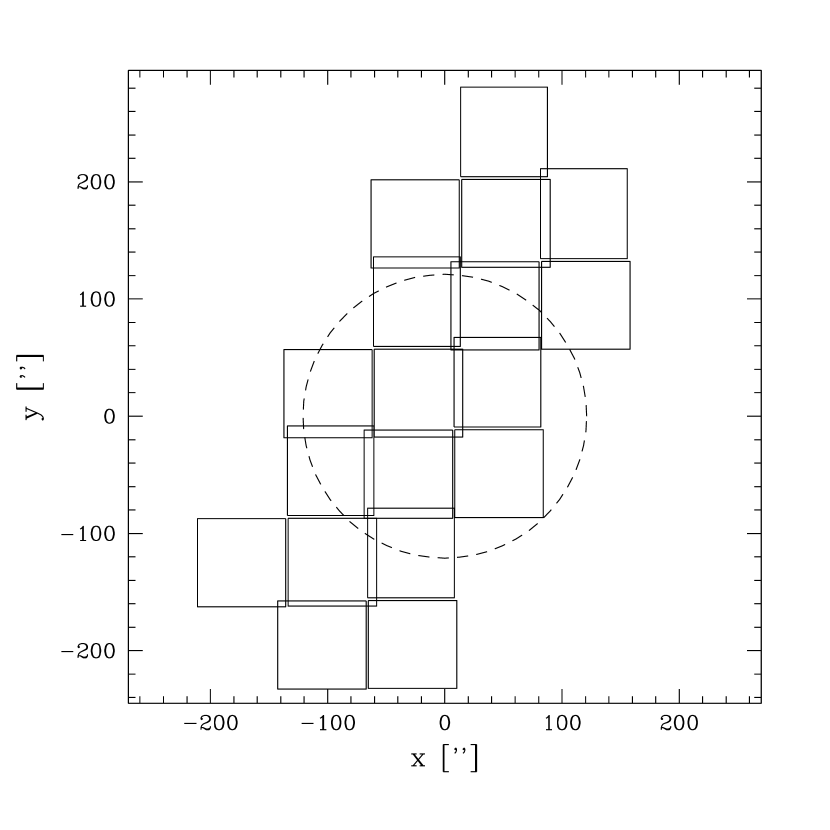
Figure 2: Layout of the observed field. The six pointings are indicated. The dashed circle indicates an aperture with a radius of $1~{}h_{50}^{-1}$ Mpc centered on the brightest cluster galaxy (BCG). The area covered by the observations is approximately 26.5 armin².

2 Data

To study the cluster MS 2053 we use a mosaic of WFPC2 images taken with the Hubble Space Telescope. Figure 2 shows the layout of the mosaic constructed from the 6 pointings of the telescope. The cluster has been observed in two passbands. Each pointing in each filter consists of three separate short exposures, which allows an effective rejection of cosmic rays. The total integration time per pointing was 3300s in the $F606W$ filter, and 3200s in the $F814W$ filter. The reduction is described in van Dokkum et al. (2001). For the weak lensing analysis we omit the data of the Planetary Camera because the data do not reach the same depth as the Wide Field Camera. The total area covered by the observations is approximately 26.5 arcmin².

Figure 4: Plot of the apparent magnitude in the $F606W$ filter (a) and the $F814W$ filter (b) versus half light radius $r_{h}$. Because of the low galactic latitude of MS 2053 many stars are found, which correspond to the vertical sequence of points at $r_{h}\sim 0\hbox{$.\!\!^{\prime\prime}$}{1}$.

3 Object analysis

The weak lensing analysis technique is based on that developed by Kaiser, Squires, & Broadhurst (1995), and Luppino & Kaiser (1997), with a number of modifications which are described in detail in HFKS and HFK. We analyse each WFPC2 chip separately, and combine the object catalogs to a master catalog once all objects have been analysed and the appropriate corrections have been applied.

We use the hierarchical peak finding algorithm from Kaiser et al. (1995) to find objects with a significance $>5\sigma$ over the local sky. These are analysed, which yields estimates for their sizes, magnitudes and shapes. As described in HFK we also estimate the error on the shape measurements, which allows a proper weighting of the sources.

The resulting catalogs are inspected visually, and spurious detections, such as diffraction spikes, HII regions in resolved galaxies, etc. are removed.

We then identify the objects that are detected in both the $F606W$ and $F814$ images. For these we determine colours using the same aperture for both filters. The aperture that is used scales with the Gaussian scale length $r_{g}$ of the object. This results in a sample of 2155 objects, both galaxies and stars, with a corresponding number density of 81 objects arcmin^-2. The objects that are detected in only one filter are small, and faint, and as a result not useful for the weak lensing analysis.

The magnitudes are zero-pointed to Vega, using the zero points given the HST Data Handbook (Voit et al. 1997). Figure 4 shows the plot of the apparent magnitude versus the object half light radius of the detected objects.

Because of the low galactic latitude of MS 2053 many stars are found in the observed field. These are located in the vertical sequence of points at a half-light radius $r_{h}\sim 0\hbox{$.\!\!^{\prime\prime}$}{1}$. The brightest stars saturate and have larger half light radii. Based on Figure 4 we select a sample of 198 moderately bright stars. These stars are used to study the PSF, and the results are used to correct the shapes of the faint galaxies for PSF anisotropy and the size of the PSF as described in HFKS.

The observed polarizations in the $F814W$ images of these stars are presented in Figure 6. HFKS studied the WFPC2 PSF using observations of the globular cluster M4, and the pattern observed here is similar to the one presented in HFKS.

The PSF changes slightly with time, and subtraction of the M4 model from the observations leaves systematic residuals. To improve the model for the PSF anisotropy we fitted a modified model to the shape parameters of the stars in the MS 2053. It is a scaled version of the M4 model with a first order polynomial added:

$$p_{i}^{\rm new}=a\cdot p_{i}^{\rm M4}+c_{0}+c_{1}x+c_{2}y.$$

This model fits the observed PSF anisotropy of stars in the MS 2053 field well (the reduced $\chi^{2}$ of the fit is 0.98 for 179 stars).

Figure 6: Observed polarization of stars selected from the $F814W$ images. The sticks indicate the direction of the major axis of the PSF, as well as the size of the polarization. The polarizations are measured using a Gaussian weight function with a dispersion of 0$.\!\!^{\prime\prime}$07. The lower left panel corresponds to chip2, the lower right to chip 3, and the upper right one denotes chip 4. We have omitted chip 1, which is the planetary camera.

The next step is to determine the “pre-seeing” shear polarizability $P^{\gamma}$ (Luppino & Kaiser 1997; HFKS). The measurements of $P^{\gamma}$ for individual galaxies are rather noisy, and therefore we bin the measurements as a function of the Gaussian scale length $r_{g}$.

Because of the poor sampling of WFPC2 images only the shapes of galaxies with size $r_{g}>0\hbox{$.\!\!^{\prime\prime}$}{08}$ can be corrected reliably. We select objects that have $r_{g}>0\hbox{$.\!\!^{\prime\prime}$}{08}$ and remove saturated stars from the catalogs. After this selection the sample of galaxies consists of 1540 galaxies analysed from the $F606W$ images, and 1545 from the $F814W$ images. We note that because of this cut not all objects appear in both catalogs anymore.

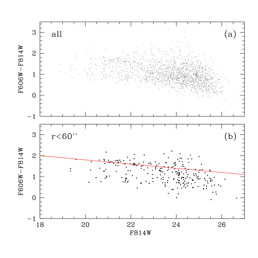
Figure 8: (a) Colour-magnitude diagram of the galaxies in the full mosaic for which colours have been determined. (b) Colour-magnitude diagram for galaxies within 1 arcminute from the BCG. The cluster colour-magnitude relation is better visible in this diagram, although it is not as obvious as for other rich clusters. The line indicates the assumed cluster colour-magnitude relation.

Finally the shapes are corrected for the camera distortion, and the catalogs are combined into a master catalog. We use the estimated errors on the shape measurements to combine the results from the $F606W$ and $F814W$ images in an optimal way. The resulting catalog includes 1677 galaxies, which corresponds to a number density of 63 galaxies arcmin^-2.

4 Light distribution

Figure 8a shows the colour of the galaxies in the full mosaic versus their $F814W$ magnitude. Compared to the other two clusters for which we obtained HST mosaics, MS 2053 is less obvious from the optical images. As a result the contrast of the cluster colour-magnitude relation with the background is lower. However, in the diagram for galaxies within 1 arminute from the BCG the cluster colour-magnitude relation can be discerned (fig. 8b).

To estimate the light contents of the cluster we define a sample of cluster galaxies as follows. Down to $F814W=21$ we select spectroscopically confirmed cluster members (Van Dokkum et al. 2001, in preparation). At fainter magnitudes we use the colour-magnitude relation drawn in Figure 8b. We select galaxies with $-0.4<\Delta(F606W-F814W)<0.2$ mag relative to the cluster colour-magnitude relation. To correct for contamination by field galaxies we subtract the counts from the Hubble Deep Fields north and south. The smoothed luminosity distribution of this sample is presented in Figure 10a. In Figures 10b and c grey scale images of the smoothed number density of bright $(19.5<F814W<23)$ and faint $(23<F814W<25)$ galaxies are presented. Around the position of the BCG a significant overdensity of galaxies is detected. Figure 10a shows most clearly that the light distribution is elongated in the direction where the arc is found (Luppino & Gioia 1992). Figure 10c still shows an overdensity at the position of the cluster. Interestingly, it also shows a clear overdensity south of the cluster. The overdensity is caused by galaxies bluer than the cluster, but it is not clear whether they belong to another cluster along the line of sight.

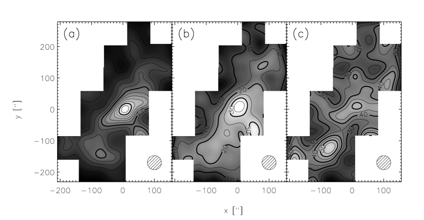
Figure 10: (a) Smoothed luminosity distribution from the sample of cluster galaxies. The definition of the sample is described in the text. The intervals between subsequent contours are $10^{6}{\rm L}_{B\hbox{$\odot$}}{\rm pc}^{-2}$. The position of the BCG has been used to define the cluster centre, and corresponds to the origin of this figure. The overdensity at the cluster centre is clearly visible. (b) Smoothed number density of bright galaxies ($19.5<F814W<23$). (c) smoothed number density of faint galaxies ($23<F814W<25$). At the position of the cluster a small overdensity is still visible. Another overdensity of faint galaxies is visible to the lower left of the cluster. The number density distributions have been smoothed using a Gaussian with a FWHM of 45” (indicated by the shaded circle). In figures (b) and (c) the intervals between subsequent contours are 5 galaxies arcmin^-2.

We estimate the cluster luminosity in the rest frame $B$ band. To do so we use template spectra for a range in spectral types and compute the corresponding pass band correction (this procedure is similar to the method described in van Dokkum & Franx 1996). Thus we find the following transformation from the HST filters to the rest frame $B$ band:

$$B_{z}=F814W+0.47(F606W-F814W)+0.75,$$

where $B_{z}$ denotes the corrected $B$ band magnitude. The luminosity is given by

$$L_{B}=10^{0.4(M_{B\odot}-B_{z}+DM+A_{F814W})}L_{B\odot},$$

where $M_{B\odot}=5.48$ is the solar absolute $B$ magnitude, $DM$ is the distance modulus, and $A_{F814W}$ is the extinction correction in the $F814W$ filter towards MS 2053. The redshift of $z=0.58$ for MS 2053 gives a distance modulus of $43.14-5\log h_{50}$. We use the dust maps from Schlegel, Finkbeiner, & Davis (1998) to correct for the galactic extinction. Because of the low galactic latitude of MS 2053, we find a rather high value of $A_{F814W}=0.15$. We have used SExtractor (Bertin & Arnouts 1996) to determine total magnitudes for the galaxies.

The cumulative light profile as a function of distance from the cluster centre is presented in Figure 12. The total luminosity within an aperture of radius $1~{}h_{50}^{-1}$ Mpc is $(3.1\pm 0.4)\times 10^{12}h_{50}^{-2}{\rm L}_{B\odot}$. The error in the luminosity reflects the uncertainty in the determination of cluster membership, and the total magnitudes measured by SExtractor. We note, however, that the error is small compared to the uncertainty in the weak lensing signal (section 4 and further). At large radii the profile is rather steep. To compute the profile, we average the light distribution in circular bins. If the light distribution is elongated as suggested by Figure 10a this leads to an overestimate of the light at large radii, where the coverage is incomplete.

5 Weak lensing signal

Each galaxy gives only a noisy estimate of the weak lensing signal because of its intrinsic shape. Therefore we average the shape measurements of many sources to obtain a useful estimate of the distortion $g$. When we compute the ensemble averaged distortion, we weight the contribution of each object with the inverse square of the uncertainty in the measurement of the distortion as described in HFK.

We select galaxies with $21.5<F814W<25.5$, and $0<F606W-F814W<1.4$ in our sample of background galaxies. As mentioned above, we exclude objects with sizes comparable to the PSF. The resulting sample consists of 1130 galaxies, and has a median magnitude of $F814W=24.3$. Comparison with Figure 8 shows that some faint cluster members might end up in this sample of background sources. The contamination will be most important in the central region of the cluster. To estimate the contamination by cluster members we examined the azimuthally averaged number density as a function of distance from the cluster centre. The profile is presented in Figure 14. The number counts are slightly higher near the cluster centre, but the excess is not significant. In the further analysis we ignore the data inside 40” from the BCG.

The average number density of sources is 43 galaxies arcmin^-2. Similar number densities can be reached in deep images taken from the ground (e.g., Bézecourt et al. 2000). However, the main advantage of our observations over ground based images is the much smaller correction for the size of the PSF. As a result the lensing signal is better calibrated, and the noise in the shape measurements from HST data is lower.

Figure 12: The cumulative restframe $B$ band luminosity as a function of radius from the cluster centre. The profile is calculated using the sample of cluster galaxies (selected both spectroscopically and based on colour). The arrow indicates a radius of $1~{}h_{50}^{-1}$ Mpc.

Figure 16a shows the smoothed distortion field from the sample of source galaxies (we used a Gaussian with a FWHM of $45^{\prime\prime}$). The position of the BCG corresponds to the origin of the plot. A systematic tangential alignment of the sources with respect to the cluster centre can be observed.

We use the distortion field presented in Figure 16a to reconstruct the projected surface mass density. The mass reconstruction has been computed using the maximum likelihood extension of the original KS algorithm (Kaiser & Squires 1993; Squires & Kaiser 1996). This algorithm has the advantage over direct inversion methods that it can be applied to fields with complicated boundaries, such as our mosaic.

Figure 16b shows a grey scale image of the reconstructed surface mass density. The peak in the mass distribution coincides with the position of the BCG. A bootstrapping resampling of the shape measurements enables us to compute the noise map of the mass reconstruction, which is presented in Figure 16c. The noise in the mass reconstruction increases rapidly towards the edges of the observed field. From the noise map we find that the peak in the mass distribution is detected at the $3\sigma$ level.

Figure 14: Azimuthally averaged number density of background galaxies ($21.5<F814W<25.5$ and $0<F606W-F814W<1.4$) as a function of distance from the cluster centre. The counts have been corrected for the boundaries of the mosaic. No significant overdensity is found at the cluster position, which indicates that the contamination by cluster members is low. The dashed line shows the average number density of 43 background galaxies arcmin.^-2

6 Mass and mass-to-light ratio

The azimuthally averaged tangential distortion $\langle g_{T}\rangle$ as a function of radius from the cluster centre is a useful measure of the lensing signal (e.g., Miralda-Escudé 1991; Tyson & Fischer 1995). The tangential distortion is defined as $g_{T}=-(g_{1}\cos 2\phi+g_{2}\sin 2\phi)$, where $\phi$ is the azimuthal angle with respect to the assumed cluster centre, for which we take the position of the BCG.

The azimuthally averaged tangential distortion as a function of radius from the cluster centre is presented in Figure 18. A singular isothermal sphere model ($\kappa(r)=r_{E}/2r$, where $r_{E}$ is the Einstein radius) gives a best fitted $r_{E}=6{\hbox{$.\!\!^{\prime\prime}$}}3\pm 1{\hbox{$.\!\!^{\prime\prime}$}}8$. To minimize the diluting effect of cluster galaxies on the weak lensing signal, we have excluded the measurements at radii smaller than 40” from the fit.

6.1 Velocity dispersion

The next step is to relate the measurement of the Einstein radius to a velocity dispersion, for which we use photometric redshift distribution from the the northern and southern Hubble Deep Fields (Fernández-Soto, Lanzetta, & Yahil 1999; Chen et al. 1998). HFK examined the usefulness of photometric redshift distributions to calibrate the lensing signal and found that they work well.

The amplitude of the lensing signal as a function of source redshift is characterized by $\beta$, which is defined as $\beta=\max[0,D_{ls}/D_{s}]$, where $D_{ls}$ and $D_{s}$ are the angular diameter distances between the lens and the source, and the observer and the source. To compute $\langle\beta\rangle$ we also take into account that fainter galaxies are noisier and have a lower weight in the average. For our sample of sources we obtain $\langle\beta\rangle=0.29$ (taking $\Omega_{m}=0.3$, and $\Omega_{\Lambda}=0$). Placing the background galaxies in a single source plane at $z=1$ would yield a similar $\langle\beta\rangle$. Using these results we derive a velocity dispersion of $\sigma=886^{+121}_{-139}$ km/s.

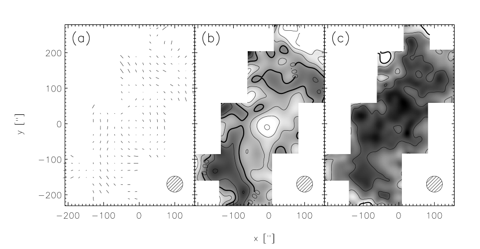
Figure 16: (a) Smoothed distortion field $g$ obtained using galaxies with $22<F814W<26$ and $0<F606W-F814W<1.6$. The measurements have been smoothed using a Gaussian with a FWHM of 45 arcseconds (indicated by the shaded circle). The orientation of the sticks indicates the direction of the distortion, and the length is proportional to the amplitude of the signal. The origin of the plot coincides with the assumed cluster centre. (b) The corresponding reconstruction of the projected surface mass density. The interval between adjactent contours is 0.05 in $\kappa$. (c) Noise map of the mass reconstruction from bootstrapping resampling of the shape measurements. It shows that the noise in the reconstruction increases rapidly towards the edges of the observed field. The interval between adjacent contours is 0.025. The peak in the mass reconstruction is detected at the $3\sigma$ level.

The value of $\langle\beta\rangle$ does not only depend on the redshifts of the sources, but it also depends on the cosmological parameters that define the angular diameter distances. For an $\Omega_{m}=1$, and $\Omega_{\Lambda}=0$ model we find essentially the same $\langle\beta\rangle$, and $\sigma=881^{+120}_{-138}$ km/s. In a $\Omega_{\Lambda}$ dominated universe the changes are larger. Assuming $\Omega_{m}=0.3$, and $\Omega_{\Lambda}=0.7$ gives $\langle\beta\rangle=0.33$, and results in $\sigma=831^{+113}_{-130}$ km/s.

The result from the weak lensing analysis is in excellent agreement with the observed velocity dispersion of $817\pm 80$ km/s, which was determined from the velocities of 52 cluster members (Van Dokkum et al. 2001, in preparation).

Clowe (1998) obtained deep $R$ band images of MS 2053 with the Keck telescope, and measured the weak lensing signal. He used a source redshift of $z=1.75$ and derived a velocity dispersion of $\sigma\sim 700$ km/s. Such high average source redshifts are unrealistic, in particular when compared to the $z=1$ we use, based on photometric redshift distributions. For more realistic redshift distributions the result of Clowe (1998) increases to $\sigma\sim 900$ km/s, in good agreement with our results.

Luppino & Gioia (1992) discovered a gravitationally lensed blue arc in deep images of MS 2053. The arc is located approximately 15 arcseconds north of the BCG. To date, the redshift of the arc is not known. If we assume a redshift of $z=2$ for the arc, and adopt a SIS model (where the position of the arc gives the Eistein radius) the corresponding velocity dispersion is about 1030 km/s. This value is higher than, but consistent with the weak lensing estimate. Moreover, if the mass distribution is elongated in the direction of the arc the strong lensing mass estimate is lowered. Figure 10a indicates that the light distribution is elongated, roughly in the direction of the giant arc. Because of the low signal-to-noise ratio of the weak lensing signal, we cannot constrain the elongation of the mass distribution.

6.2 Mass-to-light ratio

From the sample of cluster galaxies we estimate a total cluster luminosity of $(3.1\pm 0.4)\times 10^{12}h_{50}^{-2}{\rm L}_{B\odot}$ within an aperture of radius $1~{}h_{50}^{-1}$ Mpc (see section 4). The best fit SIS model gives a projected mass of $(5.7\pm 1.6)\times 10^{14}h_{50}^{-1}{\rm M}_{\odot}$ in the same aperture. Thus we obtain an average mass-to-light ratio of $184\pm 56~{}\hbox{$h_{50}~{}{\rm M}_{\odot}/{\rm L}_{{\rm B}\odot}$}$ within $1~{}h_{50}^{-1}$ Mpc.

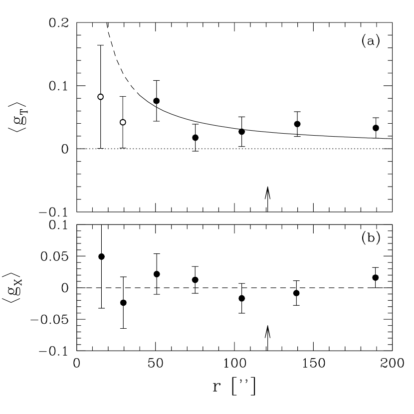
Figure 18: (a) Average tangential distortion as a function of radius from the cluster centre, for which we took the position of the brightest cluster galaxy. The line corresponds to the profile of a singular isothermal model ($\kappa(r)=r_{E}/2r$, where $r_{E}$ is the Einstein radius) fitted to the data. Because of possible contamination by faint cluster members we only fit to the data at radii larger than 40”. The best fit value for the Einstein radius is $r_{E}=6{\hbox{$.\!\!^{\prime\prime}$}}2\pm 1{\hbox{$.\!\!^{\prime\prime}$}}8$. (b) average signal when the phase of the distortion is increased by $\pi/2$. If the signal shown in (a) is caused by gravitational lensing, $\langle g_{X}\rangle$ should vanish, as is observed. In both figures, the arrows indicate a radius of $1~{}h_{50}^{-1}$ Mpc.

Kelson et al. (1997) have studied the fundamental plane of MS 2053. They find that the early type galaxies in the cluster define a clear fundamental plane. Comparison with low redshift clusters suggests that the structure of early type galaxies has changed little since $z=0.58$. Similar analyses have been performed for other clusters (e.g. van Dokkum & Franx 1996; van Dokkum et al. 1998) and have shown that the mass-to-light ratios of early type galaxies evolve with redshift, which is accounted to luminosity evolution.

As a result also the global cluster mass-to-light ratios evolve with redshift. The mass-to-light ratio of early type galaxies in MS 2053 in the $B$ band is $37\pm 4\%$ lower than present day values (Kelson et al. 1997). Under the assumption that the total luminosity of the cluster has changed by the same amount, we find an average mass-to-light within $1~{}h_{50}^{-1}$ Mpc of $291\pm 89\pm 19~{}\hbox{$h_{50}~{}{\rm M}_{\odot}/{\rm L}_{{\rm B}\odot}$}$, corrected for luminosity evolution to $z=0$. The first contribution to the error budget is the statistical uncertainty in the determination of the mass-to-light ratio, and the second contribution is due to the uncertainty in the correction for luminosity evolution.

Under the assumption that the light traces the mass we can derive the expected tangential distortion as a function of radius. To measure the mass-to-light ratio, we scale the computed tangential distortion $g_{T}^{\rm lum}$ to match the observed signal. In Figure 20a the resulting profile (solid line) is shown. The ratio of the computed and observed signal is presented in Figure 20b. Because of possible contamination by faint cluster members we exclude the points at radii less than 40” from the fit. We find that the results are consistent with a constant mass-to-light ratio with radius, and we find an average value of $195\pm 58~{}\hbox{$h_{50}~{}{\rm M}_{\odot}/{\rm L}_{{\rm B}\odot}$}$.

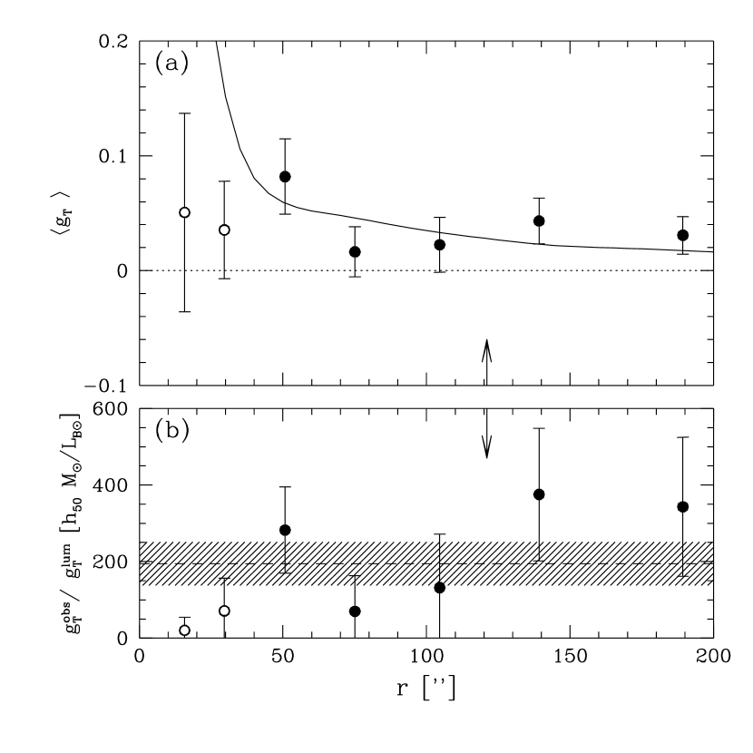
Figure 20: (a) Plot of the average tangential distortion as a function of radius from the BCG. The solid line is the expected tangential distortion (scaled by the mass-to-light ratio to fit the observations) derived from the average radial light profile, assuming the mass-to-light ratio is constant with radius. (b) The ratio of the observed distortion and the derived distortion from the light (taking $M/L_{B}=1$ in solar units). The shaded region indicates the one $\sigma$ region around the average of the points with radii larger than 40”. The observations are consistent with a constant mass-to-light ratio of $196\pm 58~{}\hbox{$h_{50}~{}{\rm M}_{\odot}/{\rm L}_{{\rm B}\odot}$}$. In both figures, the arrows indicate a radius of $1~{}h_{50}^{-1}$ Mpc.

7 Combined results from rich clusters

With the analysis of MS 2053 we have a sample of three clusters of which the mass distribution has been studied using mosaics of WPFC2 images. For the analysis in section 7.3, we augment this sample with the $z=0.22$ cluster Abell 2219, which has been studied from the ground by Bézecourt et al. (2000). Their analysis is identical to ours, and like for our clusters, photometric redshifts have been used to relate the lensing signal to the mass.

All clusters are X-ray selected, and their X-ray properties are listed in Table 2.

	$z$	$L_{x}$ (2-10 keV)	$kT$	ref.
		[$h_{50}^{-2}~{}10^{44}$ ergs/s]	[keV]
A 2219	0.22	$38$	$9.5\pm 0.6$	1
Cl 1358+62	0.33	$11.4\pm 0.3$	$6.9\pm 0.5$	2
MS 2053-04	0.58	$7.9\pm 0.7$	$8.1^{+3.7}_{-2.2}$	2
MS 1054-03	0.83	28.6	$12.4^{+3.1}_{-2.2}$	3

Table 2: X-ray properties of the three clusters for which we have obtained HST mosaics, as well as the properties of A 2219. References: (1) Allen (1998); (2) Henry (2000); (3) Donahue et al. (1998).

7.1 Comparison between weak lensing mass and dynamical mass

The large number of spectroscopic confirmed members in each of the remaining three clusters results in accurate measurements of their galaxy velocity dispersions. In this section we compare the weak lensing estimates of the cluster velocity dispersions to the velocity dispersion of the galaxies. In Table 4 we list the results of the best fit SIS model to the observed weak lensing signal, as well as the corresponding velocity dispersion inferred from lensing.

	$z$	$r_{E}$	$\langle\beta\rangle$	$\sigma$ (WL)	$\sigma$ (galaxies)	ref.
		[”]		[km/s]	[km/s]
Abell 2219	0.22	$17.4\pm 2.0$	0.46	$1075^{+61}_{-63}$	-	-
Cl 1358+62	0.33	$10.8\pm 1.4$	0.56	$835^{+52}_{-56}$	$910\pm 54$	1
MS 2053-04	0.58	$6.3\pm 1.8$	0.29	$886^{+121}_{-139}$	$817\pm 80$	2
MS 1054-03	0.83	$11.5\pm 1.4$	0.23	$1311^{+83}_{-89}$	$1150\pm 90$	3

Table 4: Results from the weak lensing analyses of the three clusters for which HST mosaics were obtained. References: (1) Carlberg et al. (1997); (2) Van Dokkum et al. (2001, in preparation); (3) van Dokkum (1999).

For all three clusters we use the photometric redshift distribution from the Hubble Deep Fields (Fernández-Soto et al. 1999; Chen et al. 1998). This lowered the $\langle\beta\rangle$ for Cl 1358 slightly compared to the value used in HFKS, and the new estimate for the weak lensing velocity dispersion is listed in Table 4.

The comparison with the velocity dispersions of cluster galaxies shows a good agreement in all three cases, suggesting that the galaxy velocity dispersions are characteristic of the cluster as a whole. Similar comparisons have been made in the past (e.g., Smail et al. 1997; Wu et al. 1998; Allen 1998). The samples of clusters used by Wu et al. (1998), and Allen (1998) are rather inhomogeneous: different methods were used for the correction of the circularization of the background sources, and no realistic redshift distributions of the sources have been used. Wu et al. (1998) and Allen (1998) find in general a fair agreement between the velocity dispersions of the galaxies and the velocity dispersions derived from weak lensing analyses.

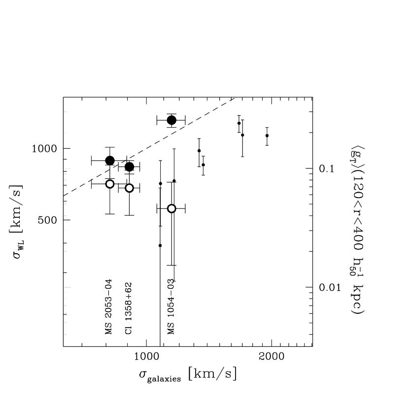
Figure 22: Weak lensing velocity dispersion (as inferred from the best fit SIS model) versus the observed velocity dispersion of the galaxies. The large open points are the results from our HST mosaics, measuring the distortion in an annulus $120<r<400~{}h_{50}^{-1}$ kpc. The results from Smail et al. (1997) are measured in the same annulus and are indicated by the small dots. The large solid points correspond to the measurements when the complete HST mosaics are used. The line of equality between the weak lensing velocity dispersion and the velocity dispersion of cluster galaxies is indicated by the dashed line. Our large field weak lensing results agree well with this line. To allow a direct comparison with Figure 4 from Smail et al. (1997) we have indicated the average tangential distortion in an annulus $120<r<400~{}h_{50}^{-1}$ on the right hand axis.

A more systematic study was presented in Smail et al. (1997) who determined the weak lensing signal of 12 distant clusters observed with WFPC2. Each cluster was observed with one pointing on the cluster core.

Smail et al. (1997) computed the average tangential distortion within an annulus $120<r<400~{}h_{50}^{-1}$ kpc, and plotted the result against the observed cluster dispersion. Under the assumption that the cluster mass distribution is described by a SIS model, this measurement provides an estimate for the velocity dispersion. Figure 22 shows the weak lensing estimate of the velocity dispersion versus the velocity dispersion of cluster members for our sample.

The large open points are the results from our HST mosaics, when we confine the weak lensing analysis to the annulus used by Smail et al. (1997). The large solid points show the results when the full HST mosaic is used for the weak lensing analysis. The right hand vertical axis displays the value of the average tangential distortion in the annulus used by Smail et al. (1997), and allows a direct comparison with their Figure 4. For comparison, we also show the results from Smail et al. (1997) (small dots).

Smail et al. (1997) found a discrepancy between their weak lensing signal and the velocity dispersion of the galaxies. They argued that the velocity dispersions from the galaxies are overestimated by $\sim 40\%$, compared to the velocity dispersion expected from the weak lensing analysis. When we confine the weak lensing analysis of our HST mosaics to the same annulus used by Smail et al. (1997) we too find that the velocity dispersion inferred from the weak lensing analysis is lower than the velocity dispersion of the galaxies. However, the results based on the full mosaics agree well with the line of equality (dashed line).

Limiting the weak lensing analysis to the cluster core results in a systematic underestimate of the cluster velocity dispersion. The largest change is seen for MS 1054. For this cluster the explanation is straightforward. HFK showed that the mass distribution in the cluster centre is complex, consisting of three distinct clumps. As a result the average tangential distortion is lowered, when only the inner $400h_{50}^{-1}$ kpc are considered in the analysis.

Several effects can introduce a systematic offset between the weak lensing results and the dynamical measurements (e.g., Smail et al 1997). Because we find a good agreement between the two estimates when the lensing signal is measured from wide field data, we argue that it is the cluster mass profile in the core that gives rise to the discrepancy. Only if the profile is isothermal, one expects a good agreement, but substrucure or a shallower density profile results lowers the lensing signal compared the value expected from the SIS model.

7.2 Average cluster mass profile

Numerical simulations have indicated that dark matter halos originating from dissipationless collapse of density fluctuations may follow a universal density profile (e.g., Navarro, Frenk, & White 1997). The Navarro, Frenk, & White (NFW) profile appears to be an excellent description of the radial mass distribution in these simulations. The NFW profile is given by

$$\rho(r)=\frac{\delta_{c}\rho_{c}}{(r/r_{s})(1+r/r_{s})^{2}},$$ (1)

where $\rho_{c}$ is the critical density of the universe, $\delta_{c}$ is the characteristic overdensity, and $r_{s}$ is the scale radius given by $r_{s}=r_{200}/c$, which all depend on the redshift and mass of the halo. The parameter $c$ is referred to as the concentration parameter. Given the cosmology, redshift, and mass of the halo, $r_{200}$ follows immediately, and the values of $\delta_{c}$, and $c$ can be computed using the routine CHARDEN made available by Julio Navarro.

We have fitted the predicted profiles from NFW halos to the observed tangential distortion of each cluster, and the best fit parameters are listed in Table 6. We have used a value of $\Gamma=0.18$ for the shape parameter of the CDM power spectrum. The parameter that we fitted is $M_{200}$, the mass enclosed within a sphere of radius $r_{200}$, and the other parameters are the ones produced by CHARDEN given $M_{200}$. The errors for $r_{200}$, $c$, and $r_{s}$ listed in Table 6 only reflect the uncertainty in these parameters because of the uncertainty in the measurement of $M_{200}$. We note that the resulting parameters are mainly determined by the amplitude of the lensing signal (i.e. the mass of the halo) and not by the shape of the density profile. Because of the strong substructure in the centre of MS 1054 we excluded the measurements at radii less than 75 arcsec.

(1)	(2)	(3)	(4)	(5)	(6)	(7)	(8)	(9)	(10)
	$z$	$M_{200}$	$r_{200}$	c	$r_{s}$	$\chi^{2}_{\rm NFW}$	$P(\chi^{2}>\chi^{2}_{\rm NFW})$	$\chi^{2}_{\rm SIS}$	$P(\chi^{2}>\chi^{2}_{\rm SIS})$
		[$10^{14}h_{50}^{-1}$ M⊙]	[$h_{50}^{-1}$ Mpc]		[$h_{50}^{-1}$ kpc]
A 2219	0.22	$16.6^{+3.4}_{-3.2}$	$2.63^{+0.17}_{-0.18}$	$5.01^{+0.13}_{-0.11}$	$524^{+47}_{-48}$	8.6	0.74	10.0	0.62
Cl 1358+62	0.33	$2.8^{+0.8}_{-0.8}$	$1.36^{+0.12}_{-0.14}$	$5.86^{+0.19}_{-0.14}$	$231^{+27}_{-31}$	15.1	0.24	15.7	0.20
MS 2053-04	0.58	$2.8^{+1.6}_{-1.5}$	$1.18^{+0.19}_{-0.27}$	$5.46^{+0.40}_{-0.22}$	$217^{+46}_{-61}$	8.6	0.74	9.6	0.65
MS 1054-03	0.83	$14.4^{+2.8}_{-2.6}$	$1.81^{+0.11}_{-0.12}$	$4.46^{+0.09}_{-0.08}$	$407^{+32}_{-34}$	11.3	0.13	11.5	0.12

Table 6: Best fit parameters for the NFW profile (columns 3-6). The fitted paramter is $M_{200}$ and the other parameters are computed using CHARDEN, for an OCDM cosmology with $\Omega_{m}=0.3$, $\Omega_{\Lambda}=0$, and shape parameter $\Gamma=0.18$. The errors indicate the 68% confidence intervals. Columns 7 and 9 give the $\chi^{2}$ for the best fit NFW profile, and SIS model, respectively. The probabilities of finding a larger value for $\chi^{2}$ are listed in columns 8 and 10.

We now examine whether the NFW predictions match the actual observations. To do so, we scale the amplitude of the tangential distortion profiles of the four clusters to the signal of a cluster with $M_{200}$ of $5\times 10^{14}h_{50}^{-1}$ M_⊙ at a redshift $z=0.5$ (where we placed the sources at infinite redshift), and scale the data radially in units of the derived value of $r_{s}$ (listed in Table 6), the scale length of the NFW profile. The resulting ensemble averaged tangential distortion as a function of $r_{s}$ is presented in Figure 24a. This figure also shows the best fit SIS model (dashed line) and the best fit NFW profile (solid line).

The NFW profile provides a good fit to the data $(\chi^{2}=12.8;~{}P(\chi^{2}>12.8)=0.38)$. The SIS model fit is worse with a $\chi^{2}=17.1$ $(P(\chi^{2}>17.1)=0.15)$. The NFW model that is fitted to the observations has a concentration parameter that is $\alpha\times c_{\rm OCDM}$. Thus we test whether the predicted concentration parameters agree with the observed lensing signal. Figure 24b shows $\Delta\chi^{2}=\chi^{2}-\chi^{2}_{\rm min}$ as a function of $\alpha$ in units of $c_{\rm OCDM}$. We find that the best fit value is $0.79^{+0.44}_{-0.15}\times c_{\rm OCDM}$. Thus the predicted concentration parameter is in good agreement with the observations.

In the above, we have used NFW models for which the parameters were obtained from the lensing data. Although the parameters are essentially determined by the amplitude of the lensing signal, it is useful to examine this in more detail. To do so, we use the observed velocity dispersions of the galaxies to obtain an estimate of $r_{200}$, using $r_{200}=(\sqrt{3}\sigma_{\rm gal})/(10H(z))$ , where $H(z)$ is the value of the Hubble parameter at the redshift of the cluster. We omit A 2219, because the galaxy velocity dispersion is not known. We compute the NFW parameters and scale the tangential distortion profiles of the three remaining clusters. The resulting ensemble averaged profile is compared to the NFW profile in the same way as before. We find that the NFW profile is a good fit $(\chi^{2}=13.4)$, and that the SIS model fits worse $(\chi^{2}=20.5)$. The best fit concentration parameter is found to be $0.83^{+0.47}_{-0.37}\times c_{\rm OCDM}$. Thus both approaches yield similar results.

These results shows that a systematic weak lensing study of a number of clusters provides a direct way to test consistency of the predictions of the theory of dissipationless collapse in CDM cosmologies.

Figure 24: (a) The ensemble averaged tangential distortion as a function of radius (in units of $r_{s}=r_{200}/c$) for the four clusters in the samples. We used the concentration parameters listed in Table 6. The solid line is the best fit NFW profile, and the dashed line is the best fit SIS model. The NFW provides the best fit $(\chi^{2}=12.8)$, whereas the SIS model fit is worse ($\chi^{2}=17.1)$. (b) $\Delta\chi^{2}=\chi^{2}-\chi^{2}_{\rm min}$ as a function of ratio between the measured and predicted concentration parameter $\alpha/c_{\rm OCDM}$. The best fit NWF profile yields an observed concentration parameter that is $0.79^{+0.44}_{-0.15}\times c_{\rm OCDM}$

7.3 Cluster mass-to-light ratio

Table 8 lists the estimates of the average mass-to-light ratio within an aperture of $1~{}h_{50}^{-1}$ Mpc radius. All values are given in the restframe $B$ band. Except for A 2219, the luminosity evolution of the early type galaxies has been measured by studying the fundamental plane (e.g., Kelson et al. 1997; Van Dokkum et al. 1998.) Under the assumption that the global cluster mass-to-light ratio evolves similarly with redshift we can correct the observed mass-to-light ratio for luminosity evolution to $z=0$, and the results are also listed in Table 8. The uncertainty in the luminosity evolution results in an additional contribution to the total error budget. In Table 8 we list the statistical error in the measurement of the mass-to-light ratio and the uncertainty due to the correction for luminosity evolution separately.

Figure 26 shows the observed average mass-to-light ratio in the $B$ band within an aperture of $1~{}h_{50}^{-1}$ Mpc as a function of cluster redshift. The dashed region in Figure 26 corresponds to the average of the observed mass-to-light ratios (i.e. assuming no luminosity evolution), which yields a value of $M/L_{B}=151\pm 12\hbox{$h_{50}~{}{\rm M}_{\odot}/{\rm L}_{{\rm B}\odot}$}$. The observations are inconsistent with an unevolving cluster mass-to-light ratio that does not evolve at the 99% level.

	$z$	${\rm M}/{\rm L}_{B}$ (obs)	${\rm M}/{\rm L}_{B}$ $(z=0)$
		[$h_{50}~{}{\rm M}_{\odot}/{\rm L}_{{\rm B}\odot}$]	[$h_{50}~{}{\rm M}_{\odot}/{\rm L}_{{\rm B}\odot}$]
A 2219	0.22	$210\pm 24$	$256\pm 29\pm 6$
Cl 1358+62	0.33	$141\pm 23$	$186\pm 30\pm 10$
MS 2053-04	0.58	$184\pm 56$	$291\pm 89\pm 19$
MS 1054-03	0.83	$124\pm 17$	$269\pm 37\pm 31$

Table 8: Average mass-to-light ratio within apertures of $1~{}h_{50}^{-1}$ Mpc radius. The error budget of the mass-to-light ratios corrected for luminosity evolution consists of the statistical uncertainty in the measurement of the mass-to-light ratio (first error) and the contritbution due to the uncertainty in the luminosity evolution (second error).

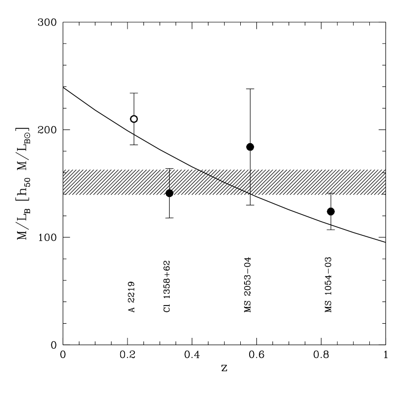
Figure 26: The observed average mass-to-light ratio within a $1~{}h_{50}^{-1}$ Mpc radius aperture of the clusters in the sample as a function of redshift. The shaded region indicates the $1\sigma$ region around the average mass-to-light ratio (assuming no luminosity evolution). The assumption of an unevolving mass-to-light ratio is excluded at the 99% confidence level. The solid line corresponds to the luminosity evolution as a function of redshift as inferred from studies of the fundamental plane of distant clusters of galaxies (Van Dokkum et al. 1998), and is consistent with the observations.

The solid line corresponds to the luminosity evolution as a function of redshift as inferred from studies of the fundamental plane of distant clusters of galaxies (Van Dokkum et al. 1998), scaled to fit the observed total cluster mass-to-light ratios. The evolution of the cluster mass-to-light ratio of X-ray selected clusters is consistent with the evolution of the mass-to-light ratio of the early type galaxies. Van Dokkum et al. (1998) found that the $M/L_{B}$ ratio evolves as $\Delta\log M/L_{B}\propto(-0.40\pm 0.04)z$, which results in an average value of $M/L_{B}=239\pm 18\pm 9\hbox{$h_{50}~{}{\rm M}_{\odot}/{\rm L}_{{\rm B}\odot}$}$ for clusters at $z=0$. The first error indicates the statistical uncertainty in the measurement of the mass-to-light ratio, and the second error indicates the additional error introduced by the uncertainty in the luminosity evolution.

Carlberg et al. (1997) analysed a sample of 16 rich clusters, and also found that the cluster mass-to-light ratios are consistent with a universal value. They found an average value of $M/L_{r}=119\pm 21~{}h_{50}{\rm M}_{\odot}/{\rm L}_{r\odot}$. To convert this value to a mass-to-light ratio in the $B$ band, we assume an average colour of the cluster of $B-r=1.07$, which corresponds to the typical colour of S0 galaxies (Jørgensen et al. 1995). Thus we find that the estimate for the average cluster mass-to-light ratio from Carlberg et al. (1997) corresponds to $219\pm 38~{}\hbox{$h_{50}~{}{\rm M}_{\odot}/{\rm L}_{{\rm B}\odot}$}$ (where we also corrected for luminosity evolution to $z=0$), in excellent agreement with our results.

Given the small spread in cluster mass-to-light ratios the star formation efficiency in rich clusters appears to be a well regulated process, although the sample of clusters needs to be increased before firmer conclusions can be drawn.

8 Conclusions

We have presented the results of our weak lensing analysis of MS 2053-04, a cluster of galaxies at a redshift $z=0.58$, for which we detect a clear lensing signal. It is the third cluster we have studied using a two-colour mosaic of deep WFPC2 images. Previously we have studied Cl 1358+62 ($z=0.33$; HFKS) and MS 1054-03 ($z=0.83$; HFK).

The selected sample of background sources (with $21.5<F814W<25.5$ and $0<F606W-F814W<1.4$) has a number density of 43 galaxies arcmin^-2. Similar number densities can be reached in deep ground based observations, but the correction for the circularization by the PSF in WFPC2 images is much smaller. As a result the lensing signal can be measured more accurately from space based images.

The position of the peak in the reconstruction of the cluster mass surface density agrees well with the peak in the light distribution. To measure the mass of the cluster we fit a SIS model to the observed azimuthally averaged tangential distortion. The corresponding value for the Einstein radius is $r_{E}=6{\hbox{$.\!\!^{\prime\prime}$}}2\pm 1{\hbox{$.\!\!^{\prime\prime}$}}8$. To relate the Einstein radius to an estimate of the cluster velocity dispersion, we use published photometric redshift distributions inferred from the northern and southern Hubble Deep Fields. The best fit SIS model corresponds to a velocity dispersion of $\sigma=886^{+121}_{-139}$ km/s, which is in excellent agreement with the observed velocity dispersion of cluster galaxies of $817\pm 80$ km/s.

We have analysed the weak lensing signal of 3 clusters using wide field HST data, and we find that the velocity dispersion derived from weak lensing agrees well with the velocity dispersion of the cluster galaxies. This result differs from Smail et al. (1997) who compared the weak lensing signal to the galaxy velocity dispersion using HST observations of cluster cores. Based on our results we argue that the discrepancy is caused by deviations from the SIS model in the inner regions of clusters (substructure or a flatter profile). To obtain an accurate estimate of the weak lensing velocity dispersion wide field data are necessary.

We use a sample of 4 clusters that have been analysed uniformly to study the average cluster profile. The NFW profile fits the ensemble averaged lensing signal well, and the predicted concentration parameter is in good agreement with the observations: the observed value is found to be $0.79^{+0.44}_{-0.15}$ times the predicted value for an OCDM model.

The observed average mass-to-light ratio of MS 2053 within a $1~{}h_{50}^{-1}$ Mpc radius aperture is $184\pm 56~{}\hbox{$h_{50}~{}{\rm M}_{\odot}/{\rm L}_{{\rm B}\odot}$}$. We have examined the mass-to-light ratios of the clusters in our sample, and find that the results are inconsistent with a non-evolving universal mass-to-light ratio. The measurements are consistent with a universal mass-to-light ratio for rich, X-ray selected, clusters of galaxies which evolves with redshift similarly to the luminosity evolution of the cluster galaxies (e.g., Kelson et al. 1997; van Dokkum et al. 1998). The average cluster mass-to-light ratio, corrected to $z=0$, is found to be $M/L_{B}=239\pm 18\pm 9~{}h_{50}~{}\hbox{$h_{50}~{}{\rm M}_{\odot}/{\rm L}_{{\rm B}\odot}$}$ (where the first error indicates the statistical uncertainty in the measurement of the mass-to-light ratio, and the second error is due to the uncertainty in luminosity evolution), in good agreement with the results from Carlberg et al. (1997) based on a dynamical study of 16 rich clusters. The small spread in cluster mass-to-light ratios suggests that the total star formation in clusters is a well regulated process.

References

- Allen 1998 Allen, S.W. 1998, 296, 392
- Bahcall & Fan Bahcall, N.A., & Fan, X. 1998, ApJ, 504, 1
- Bertin & Arnouts Bertin, E., & Arnouts, S. 1996, A&AS, 117, 393
- Bezecourt 2000 Bézecourt, J., Hoekstra, H., Gray, M.E., AbselSalam, H.M., Kuijken, K., & Ellis, R.S. 2000, A&A submitted, astro-ph/0001513
- Carlberg et al. 1997 Carlberg, R.G., Yee, H.C., & Ellingson 1997, ApJ, 478, 462
- Chen et al. 1998 Chen, H.-W., Fernández-Soto, A., Lanzetta, K.M., Pascarelle, S.M., Puetter, R.C., Yahata, N., & Yahil, A., preprint, astro-ph/9812339
- Clowe 1998 Clowe, D.I. 1998, PhD Thesis, University of Hawaii
- Della Ceca et al. 2000 Della Ceca, R., Scaramella, R., Gioia, I.M., Rosati, P., Fiore, F., & Squires, G. 2000, A&A, 353, 498
- Donahue et al. 1998 Donahue, M., Voit, G.M., Gioia, I., Luppino, G.A., Hughes, J.P., & Stocke, J.T. 1998, ApJ, 502, 550
- Eke 1996 Eke, V.R., Cole, S., & Frenk, C.S. 1996, MNRAS, 282, 263
- Fernandez-Soto et al. 1999 Fernández-Soto, A., Lanzetta, K.M., & Yahil, A. 1999, ApJ, 513, 34
- 1 Gioia, I.M., Luppino, G.A. 1994, ApJS, 94, 583
- 2 Henry, J.P. 2000, ApJ, 534, 565
- 3 Hoekstra, H., Franx, M., & Kuijken, K. 2000, ApJ, 532, 88 (HFK)
- 4 Hoekstra, H., Franx, M., Kuijken, K., & Squires, G. 1998, ApJ, 504, 636 (HFKS)
- Jorgensen et al. 1995 Jørgensen, I., Franx, M., & Kjærgaard, P. 1995, MNRAS, 273, 1097
- Kaiser & Squires 1993 Kaiser, N., & Squires, G. 1993, ApJ, 404, 441
- Kaiser, Squires & Broadhurst 1995 Kaiser, N., Squires, G., & Broadhurst, T. 1995, ApJ, 449, 460
- Kelson et al. 1997 Kelson, D.D., van Dokkum, P.G., Franx, M., Illingworth, G.D., & Fabricant, D. 1997, ApJ, 478, L13
- 5 Luppino, G.A. & Gioia, I.M. 1992, A&A, 265, L9
- Luppino & Kaiser 1997 Luppino, G.A., Kaiser, N. 1997, ApJ, 475, 20
- Mellier 1999 Mellier, Y. 1999, ARA&A, 37, 127
- Miralda 1991 Miralda-Escudé, J. 1991, ApJ, 370, 1
- NFW97 Navarro, J.F., Frenk, C.S., & White, S.D.M. 1997, ApJ, 490, 493
- Schlegel et al. 1998 Schlegel, D., Finkbeiner, D., & Davis, M. 1998, ApJ, 500, 525
- Smail et al. 1997 Smail, I., Ellis, R.S., Dressler, A., Couch, W.J., Oemler Jr., A., Sharples, R.M., & Butcher, H. 1997, ApJ, 479, 70
- Squires & Kaiser 1996 Squires, G. & Kaiser, N. 1996, ApJ, 473, 65
- Tyson & Fischer Tyson, J.A., & Fischer, P. 1995, ApJ, 446, L55
- Van Dokkum 1999 van Dokkum, P.G. 1999, Ph.D. thesis, Groningen University
- Van Dokkum & Franx 1996 van Dokkum, P.G., & Franx, M. 1996, MNRAS, 281, 985
- Van Dokkum et al. 1998 van Dokkum, P.G., Franx, M., Kelson, D.D., & Illingworth, G. 1998 ApJ, ApJ, 504, L17
- VD01 van Dokkum, P.G., Franx, M., Kelson, D.D., & Illingworth, G.D. 2001, ApJ, 553, L39
- Voit et al. 1997 Voit, M., et al. 1997, HST Data Handbook, version 3.0 (Baltimore:STScI)
- Wu et al. 1998 Wu, X.-P., Chiueh, T., Fang, L.-Z., Xue, Y.-J. 1998, MNRAS, 301, 861