Confidence levels of evolutionary synthesis models

In terms of statistical fluctuations, stellar population synthesis models are only asymptotically correct in the limit of a large number of stars, where sampling errors become asymptotically small. When dealing with stellar clusters, starbursts, dwarf galaxies or stellar populations within pixels, sampling errors introduce a large dispersion in the predicted integrated properties of these populations. We present here an approximate but generic statistical formalism which allows a very good estimation of the uncertainties and confidence levels in any integrated property, bypassing extensive Monte Carlo simulations, and including the effects of partial correlations between different observables. Tests of the formalism are presented and compared with proper estimates. We derive the minimum mass of stellar populations which is required to reach a given confidence limit for a given integrated property. As an example of this general formalism, which can be included in any synthesis code, we apply it to the case of young ($t\leq 20$ Myr) starburst populations. We show that, in general, the UV continuum is more reliable than other continuum bands for the comparison of models with observed data. We also show that clusters where more than 10⁵ M_⊙ have been transformed into stars have a relative dispersion of about 10% in Q(He⁺) for ages smaller than 3 Myr. During the WR phase the dispersion increases to about 25% for such massive clusters. We further find that the most reliable observable for the determination of the WR population is the ratio of the luminosity of the WR bump over the H$\beta$ luminosity. A fraction of the observed scatter in the integrated properties of clusters and starbursts can be accounted for by sampling fluctuations.

1 Introduction and motivation

In the past few years, the increasingly detailed observations of stellar populations in a wide variety of environments – from stellar clusters to high redshift galaxies – has driven the development of increasingly complicated evolutionary synthesis codes. A great care has been given to the use of updated physical ingredients (like more realistic model atmospheres, grids of observed spectra, stellar tracks covering more evolutionary phases, increased wavelength range, etc) and technical details (interpolation methods, convolutions, etc), leading to a situation where the outputs produced by different codes are roughly consistent with each other, although they perhaps disagree on the interpretation of a given observable. Systematic internal errors can be addressed comparing the outputs resulting from different inputs or assumptions in a given code (e.g., Bruzual 2001), while the cross-comparison of different codes with the same inputs gives an estimate of the external errors (e.g., Leitherer et al. 1996).

In contrast, the study of statistical errors has received comparatively little attention, even though it seems likely that the observed scatter in the observed properties of systems with a relatively small number of stars (stellar clusters, starbursts, dwarf galaxies or stellar populations in pixels), can be accounted for by sampling fluctuations from a given (and perhaps universal) stellar initial mass function (IMF).

In this context, Barbaro & Bertelli (1977) pioneered the estimation of the dispersion of observables in stellar clusters by computing Monte Carlo simulations constrained to contain a given number of post- main sequence (PMS) stars (so as to reproduce the number of observed PMS stars in the colour-magnitude diagram of a given cluster). They concluded that under the assumption of a Salpeter IMF, the observed scatter in the integrated colours of young open clusters could be reproduced by their models. Updated analyses, by Chiosi, Bertelli & Bressan (1998), Girardi & Bica (1993) and Brocato et al. (1999) among others, yield the same results: the dispersion in a colour-colour or colour-magnitude diagram can be accounted for by these stochastic effects, at least in part.

At older ages, the presence of a few cool but very luminous stars produces the same effects. In the near-infrared, the small number of thermally pulsating AGB stars can produce strong fluctuations in the JHK bands, as pointed out by Santos & Frogel (1997) (see also Lançon and Mouhcine 2000, for a dissenting view). Even in the optical bands, the integrated colours of globular clusters can be strongly influenced by the presence of post AGB stars, as Brocato et al. (1999) have shown.

A similar problem arises when dealing with stellar populations in pixels, particularly in images or frames of nearby galaxies where each pixel could include a limited number of stars which however account for most of a given observable. See Buzzoni (1993) and Renzini (1998) for further details.

In the context of starbursts, Mayya (1995) performed a similar analysis, this time constraining the number of main sequence stars with spectral type earlier than O4, finding that while the errors in colours were larger when red supergiants appeared, they decreased when the mass of the cluster increased, being negligible for clusters more massive than about 10⁵ $M_{\odot}$.

There is, however, no systematic study of the effects of these sampling fluctuations on the integrated properties (such as colours or equivalent widths of emission and absorption lines) of simple stellar populations. Buzzoni (1989) pioneered this field by presenting a simple formalism based on Poissonian errors, and applied it to synthesis models of old stellar populations. Although powerful, this formalism does not account for some important sources of errors and is not entirely rigorous.

While it is clear that the foreseen improvements in synthesis codes will attempt to refine their realism, the detailed comparison with observed properties will still suffer from the limited number of stars which contribute to some observables. The present paper is the second of a series whose objective is to study the accuracy of evolutionary synthesis models when compared with observational data, and to point out the oversimplifications used in such models. This on-going project reviews current problems in synthesis codes and shows possible ways to overcome them, providing a guideline to include improvements in any synthesis code.

The first paper (Cerviño et al. 2000) pointed out the problem of confidence limits in synthesis models set by the presence of statistical fluctuations in the IMF, where the fluctuations were estimated by Monte Carlo simulations. In this work we present a statistical formalism to estimate quantitatively the fluctuations expected in some of the most relevant observables, and apply it, as an illustrative example, to the case of young stellar populations (ages smaller than 20 Myr), produced by statistical fluctuations in the IMF. The effect of Poissonian statistics on time-integrated observables such as supernovae rates, integrated mechanical energy output and chemical yields, as well as major problems in the time interpolations used in synthesis codes, are addressed in a third paper (Cerviño et al. 2001b). Improvements in track interpolation techniques will be discussed in a forthcoming paper. We will complete the series by extending the results presented in this paper to different star formation scenarios.

The structure of the paper is the following. In Sect. 2 we present our statistical formalism, which can be implemented in any synthesis code. In Sect. 3 we use the formalism to derive the dispersion of some relevant observables of young star-forming regions, highlighting the importance of a proper use of covariance factors in the evaluation of the dispersion. In Sect. 4 we compare the analytical dispersion and confidence levels obtained with our formalism with the ones obtained via Monte Carlo simulations. We discuss the results and draw our conclusions in Sect. 5. In Appendix A we detail error propagation in observables, giving practical examples. All the results of the paper are available from our web server at http://www.laeff.esa.es/users/mcs.

2 On sampling and Poissonian fluctuations

Let us assume that $N_{\mathrm{tot}}$ stars are observed, with masses distributed between $m_{\mathrm{low}}$ and $m_{\mathrm{up}}$. The mass $m_{i}$ of the $i$-th star is a random variable whose probability distribution function is given by $\Phi(m_{i})$ the stellar initial mass function. That is,

$$\int_{m_{\mathrm{low}}}^{m_{\mathrm{up}}}\;\Phi(m)\;dm\;\equiv\;1$$ (1)

For the case of a single power law IMF in that mass range, $\Phi(m)\sim m^{-\alpha}$, so that masses can be generated by a simple transformation from a random variable $u$ uniformly distributed in the interval $[0,1]$ with

$$m\;=\;\left[(1-u)\,m_{\mathrm{low}}^{1-\alpha}\;+\;u\,m_{\mathrm{up}}^{1-\alpha}\right]^{1/(1-\alpha)}$$ (2)

and similarly for piece-wise power laws in different mass ranges. Codes which use Monte Carlo sampling of the IMF must follow the evolution of each star generated in this way.

The number $N_{i}$ of stars of mass $m_{i}$ is another random variable, whose distribution function follows Poisson statistics. That is, the only parameter of the Poisson distribution is precisely the value of the IMF at that mass

$$dn_{i}\,=\,dN_{i}\,/\,N_{\mathrm{tot}}\;=\;\Phi(m_{i})\,dm_{i}$$ (3)

since obviously the total number of stars is $\int dN_{i}\equiv$ $N_{\mathrm{tot}}$. Note that stellar evolution does not change the Poissonian nature of $N_{i}$, and that the normalised random variable $n_{i}$ is almost a Poisson variable, since the ratio of a Poisson variable with a constant is not necessarily a Poisson variable (e.g., Kendall & Stuart 1977).

A simple test to check the Poissonian nature of the distribution of $n_{i}$ is simply the ratio of its variance $\sigma^{2}(n_{i})$ to its average value $\mathopen{<}n_{i}\mathclose{>}$ as a function of mass $m_{i}$. This ratio should be close to unity for the entire range of masses considered. The situation is illustrated in Fig. 1 with 1000 Monte Carlo simulations of clusters with $10^{3}$ and $10^{4}$ stars with a Salpeter IMF slope ($\alpha=2.35$) in the mass range 2 – 120 M_⊙. Figure 1 shows that despite the fact that $n_{i}$ is the ratio of a Poisson variable with a constant, it is Poisson-distributed to within 10% even in clusters with as few as $N_{\mathrm{tot}}$= 10³ stars. Note that codes which use a binning in mass must ensure that the size of the bins is small, otherwise the correlations induced may produce a systematic effect, especially for the lower mass stars, as shown on Fig. 1.

Figure 1: Ratio of variance over mean value as a function of mass for 1000 Monte Carlo simulations with $N_{\mathrm{tot}}$  = $10^{3}$ stars (upper panel) and $N_{\mathrm{tot}}$  = $10^{4}$ stars (lower panel). Solid line: $\sigma^{2}(n_{i})/n_{i}$ using a mass-bin of 0.5 M_⊙ for the entire mass range. Triangles: $\sigma^{2}(n_{i})/n_{i}$ using a mass bin of 0.5 M_⊙ in the mass range $[5,120]$ M_⊙, and a mass bin of 0.01 M_⊙ when $2\mathrm{M}_{\odot}<m<5\mathrm{M}_{\odot}$.

The fact that $n_{i}$ can be approximated by a Poisson variable makes it possible to apply a proper statistical formalism, although it is slightly more subtle than one could naively expect. Take for instance the integrated monochromatic luminosity ${\cal L}_{\lambda}$ of the stellar population of $N_{\mathrm{tot}}$  stars at some wavelength $\lambda$ at some age $t$. This is simply given by the linear combination of individual monochromatic luminosities $\ell_{\lambda\,i}$ of stars of mass $m_{i}$ at the evolutionary stage of age $t$:

$${\cal L}_{\lambda}(t)\;=\;N_{\mathrm{tot}}\,\sum_{i=1}^{N_{\mathrm{tot}}}\,n_{i}\,\ell_{\lambda\,i}(t)$$ (4)

For a given age $t$, $\ell_{\lambda\,i}$ is a constant, so that ${\cal L}_{\lambda}$ is a weighted sum of Poisson-distributed random variables, and would itself be a Poisson variable if the weights would take integer values, since the sum of Poisson variables is also a Poisson variable. Hence define $\mathrm{B}_{\lambda}$ as

$$\mathrm{B}_{\lambda}\,=\,1\,+\mathrm{int}\left[\mathrm{min}\left(\ell_{\lambda\,i}\right)\right]$$ (5)

so that

$${\cal L}_{\lambda}(t)\;=\;N_{\mathrm{tot}}\,\left(1+\mathrm{B}_{\lambda}\right)\;\sum_{i=1}^{N_{\mathrm{tot}}}\,n_{i}\,\frac{1+\mathrm{int}\left(\ell_{\lambda\,i}(t)\right)}{1+\mathrm{B}_{\lambda}}$$ (6)

In this case, and up to a constant, ${\cal L}_{\lambda}$ would be a proper Poisson variable, the (integer) sum of Poisson variables, with parameter given by the sum of the individual Poisson parameters. However, as long as we are interested in dispersions and not actual distribution functions, we can disregard the actual distribution function of ${\cal L}_{\lambda}$ as long as it is a linear combination of random variables. It is convenient to introduce at this stage the random variable

$$w_{i}\;\equiv\;n_{i}\,N_{\mathrm{tot}}\,/M_{\mathrm{tot}}\;=\;N_{i}\,/\,M_{\mathrm{tot}}$$ (7)

which gives the normalised mean value of the number of stars of mass $m_{i}$ to the total mass of the cluster $M_{\mathrm{tot}}=\sum m_{i}$ assumed to be a constant. The integrated monochromatic luminosity per unit stellar mass, or specific luminosity, is

$${\mathrm{L}}_{\lambda}\;=\;{\cal L}_{\lambda}\;/\;M_{\mathrm{tot}}$$ (8)

With this notation, the expectation value of ${\mathrm{L}}_{\lambda}$ at some age $t$ becomes

$$\mathopen{<}{\mathrm{L}}_{\lambda}\mathclose{>}\;=\;\sum_{i}\,w_{i}\,\ell_{\lambda\,i}$$ (9)

The actual integrated specific luminosity ${\mathrm{L}}_{\lambda}$ will fluctuate around this average value with a variance given by

$$\mathrm{var}({\mathrm{L}}_{\lambda}) = \;\mathopen{<}\left({\mathrm{L}}_{\lambda}-\mathopen{<}{\mathrm{L}}_{\lambda}\mathclose{>}\right)^{2}\mathclose{>}\;$$ (10)

$$= \;\sum_{i}\,w_{i}\,\ell_{\lambda\,i}^{2}\;+\;\sum_{i\not=j}\,\ell_{\lambda\,i}\,\ell_{\lambda\,j}\,\mathrm{cov}(w_{i},w_{j})$$

where the covariance is given, as usual, by

$$\mathrm{cov}(w_{i},w_{j})\;\equiv\;\mathopen{<}\left(w_{i}-\mathopen{<}w_{i}\mathclose{>}\right)\,\left(w_{j}-\mathopen{<}w_{j}\mathclose{>}\right)\mathclose{>}\;$$ (11)

Note that Eq. 10 is an exact result since ${\mathrm{L}}_{\lambda}$ is a linear function of $w_{i}$. The random variables $w_{i}$ and $w_{j}$ are independent, so their covariance vanishes. Note however that codes which produce bins of mass and follow the average evolution in that bin introduce a non-zero covariance which must be taken into account, particularly if the bin size is large. We have performed several tests with different mass binning, and found that when the mass bin is smaller than 0.5 M_⊙, the covariance terms can be neglected for M$>$5 M_⊙. Furthermore, if the mass bin is made less or equal to 0.1 M_⊙, the covariance terms also vanish in the mass range 2–5 M_⊙.

So far, we have shown that ${\mathrm{L}}_{\lambda}$ (derived from ${\cal L}_{\lambda}$) is almost a Poisson variable, so we may expect its variance $\sigma^{2}({\mathrm{L}}_{\lambda})$ to be similar to its mean. This will not be exactly so, as discussed above. There are two possibilities here. The first one is to assume that the Poisson distribution is a good approximation to the distribution of ${\mathrm{L}}_{\lambda}$. In this case, we can derive approximate confidence limits in the standard way (e.g., Gehrels 1986) and then infer confidence limits for derived quantities, such as magnitudes, colours, equivalent widths, etc. This proves to be rather cumbersome. The second possibility is to disregard the actual distribution function of the specific integrated monochromatic luminosity, and deal with variances only, which can then be propagated for any derived quantity (see Appendix A).

In this context we can introduce, following Buzzoni (1989), the concept of an effective number of stars $N_{\mathrm{eff}}^{*}({\mathrm{L}}_{\lambda})$, from the relative error in the integrated monochromatic luminosity

$$\frac{1}{\sqrt{N_{\mathrm{eff}}^{*}(\mathrm{L}_{\lambda})}} = \frac{{\mathrm{var}}({{\mathrm{L}}_{\lambda}})^{1/2}}{{\mathrm{L}}_{\lambda}}=\frac{\left(\sum_{i}\mathrm{var}(w_{i})\ell_{\lambda\,i}^{2}\right)^{1/2}}{\sum_{i}w_{i}\ell_{\lambda\,i}}=$$ (12)

$$= \frac{1}{\sqrt{M_{\mathrm{tot}}}}\frac{(\sum_{i}w_{i}\ell_{\lambda\,i}^{2})^{1/2}}{\sum_{i}w_{i}\ell_{\lambda\,i}}$$

where we have made use of the fact that ${\mathrm{var}}(w_{i})=\mathrm{var}(N_{i})/M_{\mathrm{tot}}^{2}=w_{i}/M_{\mathrm{tot}}$ given that it is approximately Poisson. Even if the distribution function is not Poisson, one can still define this effective number as an approximate Poisson dispersion.

As Buzzoni (1989) emphasized, $N_{\mathrm{eff}}^{*}$ does not correspond to a real number of stars, but rather to an estimation of the relative error, in the Poisson limit. It can be interpreted as a number of contributors to a given wavelength at that age, so that if this number is small, we may expect large fluctuations in the mean value of the luminosity at this wavelength. In the case where all the stars have the same luminosity, $\ell_{\lambda\,i}=l_{\lambda}$, and since $\sum w_{i}=$ $N_{\mathrm{tot}}$  /$M_{\mathrm{tot}}$ then $N_{\mathrm{eff}}^{*}({\mathrm{L}}_{\lambda})=N_{\mathrm{tot}}$, and all stars contribute the same, obviously. In the general case, however, $N_{\mathrm{eff}}^{*}({\mathrm{L}}_{\lambda})$ can never exceed $N_{\mathrm{tot}}$, by definition. Hence small values indicate that the average value must be interpreted with caution, the variance around the mean value being as large as the mean value, typically. The ratio $N_{\mathrm{eff}}^{*}({\mathrm{L}}_{\lambda})/N_{\mathrm{tot}}$ can also be interpreted as a measure of the statistical entropy of the $\ell_{\lambda\,i}$ values (Buzzoni 1993): for a given $M_{\mathrm{tot}}$, a larger value of $N_{\mathrm{eff}}^{*}({\mathrm{L}}_{\lambda})$ means a lower dispersion in $\ell_{\lambda\,i}$. We can also rescale $N_{\mathrm{eff}}^{*}$ to the total mass in stars, following the convention used in population synthesis :

$$N_{\mathrm{eff}}=N_{\mathrm{eff}}^{*}\;/\;M_{\mathrm{tot}}$$ (13)

and the definition of $N_{\mathrm{eff}}^{*}$ can be generalized to almost all observables of a synthetic population (ratios, equivalent widths, colours etc., see Appendix A for more details). This formulation has two main advantages:

• For a cluster of a given mass, $N_{\mathrm{eff}}$ gives a simple and easy to estimate measure of the expected dispersion of a given observable. This dispersion depends on the number of stars in the cluster which effectively contributes to that observable. It must always be computed if a meaningful comparison with observed quantities of clusters of that mass is made.

• The comparison of the different values of $N_{\mathrm{eff}}$ for different observables (say, luminosities in two different passbands) gives a direct estimation of the difference in the statistical entropy of the observables, which helps to establish which observable is more reliable and thus better constrained by observations.

The $N_{\mathrm{eff}}$ formalism can, and should, be included in any synthesis code, and the corresponding values of $N_{\mathrm{eff}}(\mathbf{x})$ must be given along with every computed observable $\mathbf{x}$ so that the dispersion in $\mathbf{x}$ can be assessed. Before addressing the comparison of the dispersions computed with this analytical formalism with the ones obtained more precisely via Monte Carlo simulations in Sect. 4, it is worth giving a practical example of its application.

3 A worked example : the case of young starbursts

The first application of a simplified version of this formalism was made by Buzzoni (1989, 1993) in his study of old stellar populations, where the presence –or otherwise– of some evolutionary phases affected important observables in the optical (see also Lançon and Mouhcine (2000) for the case of infrared colours). Rapid evolutionary phases also occur in young starburst populations, and so as an illustration of the usefulness of the formalism, we apply it here to an updated version of the code presented in Mas-Hesse and Kunth (1991); Cerviño and Mas-Hesse (1994); Cerviño et al. (2001a). The main updates to the code include the following :

1. Inclusion of the full set of Geneva evolutionary tracks including standard and enhanced mass-loss rates (Meynet et al. 1994).

2. Inclusion of metallicity-dependent atmosphere models for normal stars from Kurucz and CoStar (Schaerer & De Koter 1997) and the atmosphere models for WR stars from Schmutz et al. (1992).

3. Inclusion of an analytical IMF formulation using a modified dynamical mass-bin from the Dec. 2000 release of Starburts99 (Leitherer et al. 1999). We have also kept the original Monte Carlo formulation. The dynamical mass-bin subroutine used here makes use of a more restrictive mass binning than the one used in Starburts99 with a higher numerical precision in order to ensure a narrow enough mass bin for the computation of the dispersion. The typical size of the dynamic mass bin used in our code is 10⁴ mass points. This numerical resolution does not produce however any significant changes in the mean properties obtained by both codes.

4. Use of parabolic interpolations in time for the computation of the isochrones (see Cerviño et al. 2001b, Paper iii of this series, for a full study and justification).

The code also includes an intermediate track that takes into account the discontinuity in the evolution of WR and non-WR stars. Such an intermediate track was introduced by Cerviño and Mas-Hesse (1994) and will be discussed in Paper iv of this series.

The complete predictions of the updated set of evolutionary synthesis models will be presented elsewhere. For the present example we will focus on solar metallicity simple stellar populations with standard mass-loss rates (Schaller et al. 1992), a Salpeter IMF slope in a mass range 2 – 120 M_⊙, an Instantaneous Burst star-formation law and ages from 0 to 20 Myr. We will use throughout this work an analytical approximation of the IMF, we will not use the intermediate tracks mentioned above, and we will neglect the presence of binary systems, so that our dispersion estimates can be compared to those obtained by other synthesis codes with similar inputs.

In the following subsections we discuss the dispersion estimated for a few observables predicted by the code: continuum luminosities, V–K colour, H$\beta$ equivalent width and some WR ratios. We focus here on the evolution of the dispersion of these observables, but we also show their general evolution in order to understand their dispersion. A detailed study of the evolution of these observables has been discussed elsewhere (see Cerviño and Mas-Hesse (1994) for a more detailed description of the evolution, and Leitherer & Heckman (1995), for a comparison with other synthesis models, showing that both codes give quite similar results).

3.1 Continuum properties

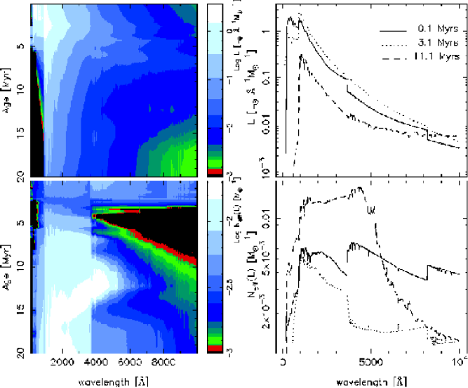
Figure 2: Specific continuum flux. Top left: Evolution of the overall spectrum. Units are L_⊙ Å^-1 M${}_{\odot}^{-1}$. Bottom left: Effective number of stars for the specific flux, in units of M${}_{\odot}^{-1}$, for the overall spectrum. The right panels show the same quantities for selected ages.

Equation 12 can be applied in a straightforward way to the continuum predicted by the synthesis code. We only need to take into account that each $\ell_{\lambda\,i}$ is the luminosity of a star of initial mass $m_{i}$ with a relative weight given by $w_{i}$.

A small complication arises in the case of young star-forming regions in that each massive star also contributes to the ionisation of the cloud around the cluster, and thus to the nebular continuum. This contribution depends on the properties of the gas in the nebula (the electronic temperature $T_{\mathrm{e}}$, the electronic density $n_{\mathrm{e}}$, and the metallicity, in the simplest case). We have used in the following the same inputs as Mas-Hesse and Kunth (1991): $T_{\mathrm{e}}=10^{4}$K, $n_{\mathrm{e}}=100\,{\mathrm{c}m}^{-3}$ and N(He ii)/N(H ii) = 0.1. We have also assumed that only a fraction $f=$0.7 of the ionising photons is absorbed by the gas.

In this case the luminosity $\ell_{\lambda\,i}$ at a given wavelength has two components, i.e. $\ell_{\lambda\,i}=l_{*,i}+l_{n,i}$ where $l_{*,i}$ is the stellar luminosity, and $l_{n,i}$ is the contribution of the star to the nebular continuum. The scaled variance in the total (stellar plus nebular) specific luminosity is then

$$\sigma_{\mathrm{L}_{\mathrm{tot}}}^{2} = \mathrm{var}(\mathrm{L}_{\mathrm{tot}})\,M_{\mathrm{tot}}^{-1}=\sum_{i}w_{i}\,\ell_{\lambda\,i}^{2}=$$ (14)

$$= \sum_{i}w_{i}l_{*,i}^{2}+\sum_{i}w_{i}l_{n,i}^{2}+2\,\sum_{i}w_{i}l_{*,i}l_{n,i}$$

The last term of the equation is the covariance between stellar and nebular continua for a given mass or star $i$ :

$${\mathrm{cov}}({\mathrm{L}}_{*},{\mathrm{L}}_{n})=\sum_{i}\,w_{i}\,l_{*,i}\,l_{n,i}.$$ (15)

Note also that the scaled dispersion of the specific monochromatic luminosity $\sigma(\mathrm{L}_{\mathrm{tot}})$ has units of erg s^-1 Å^-1 M${}_{\odot}^{-1/2}$.

The overall evolution of the continuum from 100 Å to 10⁴ Å is illustrated in the upper left panel of Fig. 2. At the beginning of the burst, massive stars are the dominant source of luminosity from the UV to the near infrared. The extreme-UV continuum (below 500 Å) appears with the first WR stars (at about 2.5 Myr) and lasts until the end of the WR phase (at about 5 Myr). The lower left panel shows the evolution of $N_{\mathrm{eff}}({\mathrm{L}}_{\lambda})$ as a function of age and wavelength. The figure shows that the extreme-UV continuum produced by WR stars has a very small $N_{\mathrm{eff}}(\mathrm{L}_{\lambda})$ value, reflecting small number statistics and the statistical entropy of the luminosities of these stars in the synthetic cluster at these wavelengths. It also shows a large dispersion in the optical and near infrared fluxes at ages between 2.5 Myr and 8.5 Myr.

The evolution of the continuum for some selected ages and the corresponding $N_{\mathrm{eff}}(\mathrm{L}_{\lambda})$ values are shown on the right panels of Fig. 2. The comparison of the lower right panel with Fig. 2 of Buzzoni (1989) is interesting. Buzzoni presents $N_{\mathrm{eff}}(\mathrm{L}_{\lambda})$ for a 15 Gyr synthetic cluster, showing an abrupt change in $N_{\mathrm{eff}}(\mathrm{L}_{\lambda})$ at the Balmer jump. In spite of the differences in the synthesis codes, ages and metallicity, the same pattern is found in our Fig. 2. The comparison of both figures reveals however the different nature of the Balmer discontinuity for stellar clusters with different effective temperatures. In clusters dominated by hot massive stars, the blue continuum is dominated by the nebular emission and is more luminous than the red continuum, while clusters with cooler stars show the opposite behaviour. This means that the discontinuity in $N_{\mathrm{eff}}(\mathrm{L}_{\lambda})$ at the Balmer jump reflects the increase in the statistical entropy of the luminosities of the stars (including the stellar and the nebular contributions) at this wavelength. At small ages (0.1 Myr), the cluster is dominated by hot stars, emitting shortwards of the Balmer continuum: the statistical entropy for $\lambda<\lambda({\rm Bac})$ is lower than that found at $\lambda>\lambda({\rm Bac})$. At 3.1 Myr, the nebular contribution to the continuum decreases rapidly. The stellar continuum contributes most to the total flux so that the statistical entropy for $\lambda<\lambda({\rm Bac})$ becomes now larger than at $\lambda>\lambda({\rm Bac})$. At 11.1 Myr, the remaining stars are so cool that the nebular emission no longer plays a role in the Balmer discontinuity. At older ages (cooler stars) the Balmer discontinuity appears completely inverted. Let us illustrate this in more detail by studying the correlation of the stellar and nebular fluxes :

• For a 0.1 Myr cluster, the nebular emission contributes more than 30% to the total (stellar + nebular) flux at wavelengths longwards $\sim$ 4000 Å. The emission at such wavelengths is therefore correlated with the ionising flux of the stars which dominate the emission at shorter wavelengths, and so $N_{\mathrm{eff}}(\mathrm{L}_{\lambda})$ is essentially flat.

• At 3.1 Myr, the nebular emission contribution at 4000 Å drops to 5%. The correlation with the ionising flux of massive stars disappears and this is reflected by a decrease in the value of $N_{\mathrm{eff}}(\mathrm{L}_{\lambda})$. Also, the emission of the different massive star populations (i.e. the $\ell_{\lambda\,i}$ values) is very variable and depends strongly on the amount of stars that become WRs. Such a situation produces a large dispersion in the ionising, optical and infrared continua.

• The dispersion in the ionising continuum vanishes at ages older than 5 Myr (when the WR population disappears), but remains large in the optical and infrared continua due to the presence of red supergiant (RSG) stars. Note that WRs and RSGs have a rapid evolution, they are very luminous, and a small amount of these stars may dominate the overall continuum. As long as their total number is small, the intrinsic dispersion at such phases of the evolution of the cluster will be large.

• Finally, a 11.5 Myr old cluster shows a small Balmer jump, and all the stars in the cluster have “similar” UV spectra, i.e. $N_{\mathrm{eff}}(\mathrm{L}_{\lambda})$ reaches a maximum value at this wavelength. The spectrum of the individual stars becomes more and more different towards the red, as shown by the decay of $N_{\mathrm{eff}}(\mathrm{L}_{\lambda})$ at longer wavelengths.

In general, the UV continuum has a larger $N_{\mathrm{eff}}(\mathrm{L}_{\lambda})$ value than the optical continuum (and thus a larger statistical entropy). This also reflects the fact that the UV continuum is more homogeneous along the spectral types, i.e. small differences in effective temperature lead to similar UV spectra. The optical continuum depends more on the effective temperature, and so small variations in the population produce larger effects. Such a dependence becomes more and more important towards longer wavelengths.

At the other extreme of the wavelength range, in the ionising continuum, the situation is even more dramatic than at IR wavelengths. The differences in the ionising continua of different stars are generally quite large, and so this part of the continuum will be the most affected by statistical fluctuations, as shown below.

3.2 Ionising continuum

We have calculated the predicted ionising flux shortwards of the He⁺, He⁰ and H⁰ edges, Q(He⁺), Q(He⁰), and Q(H⁰) respectively. The corresponding values as well as $N_{\mathrm{eff}}$(Q) and $\sigma$(Q) are shown in Fig. 3. As before, the values shown in Figure 3 are normalised to the total mass transformed into stars $M_{\mathrm{tot}}$.

Figure 3: Ionising photons. Top left: Evolution of the specific number of emitted ionising photons able to ionize He⁺, Q(He⁺), He⁰, Q(He⁰), and H⁰, Q(H⁰), in units of photons s^-1 M${}_{\odot}^{-1}$. Bottom left: Effective number, in units of M${}_{\odot}^{-1}$, for the different ionising photons (see text for definition). The right axis shows the minimum mass required to ensure a Poissonian dispersion smaller than 10% assuming a mass range 2 – 120 M_⊙ with a Salpeter IMF slope. Top right: $\sigma$(Q) in photons s^-1 M${}_{\odot}^{-0.5}$ units for the same quantities.

An important quantity in this context is the minimum mass of the cluster required to ensure a dispersion smaller than 10% in a given observable, M_10%. Clusters with smaller masses will have a dispersion larger than 10% in that observable. For instance, the right axis in the bottom left plot of Fig. 3 gives the mass of the ensemble of stars required to ensure a dispersion in the $Q$ values lower than 10%, denoted as M_10%(Q). Note that the relation between the numbers of stars present $N_{\mathrm{tot}}$ and the total mass of the cluster depends on the IMF and the mass limits adopted, and so the values of M_10% must be rescaled if different assumptions are made regarding these values.

Note that the scaled dispersion $\sigma$(Q) is larger than the normalised value of Q. It does not mean that we can obtain negative values of Q, because the probability density distribution is quasi-Poisson, i.e. the mean value and the corresponding error is not Q$\pm\sigma$(Q). Take for instance an extreme example, a cluster with a total mass $\mathrm{M}_{\mathrm{tot}}=120\mathrm{M}_{\odot}$ made up by stars with masses in the range 2–120 M_⊙ at an age of 0.1 Myr. The predicted value of the scaled (specific) average of Q(H⁰) is 4$\times 10^{47}$ photons s^-1 M${}_{\odot}^{-1}$, i.e. the actual value of Q(H⁰) for such a cluster would be 4.8$\times 10^{49}$ photons s^-1. But the actual Q(H⁰) may vary between 0 photons s^-1 (if none of the stars in the cluster produce the ionising flux) and $\sim 5\times 10^{50}$ photons s^-1 (if the cluster is formed by only one star of 120 M_⊙). In fact, the model predictions at the 90% confidence level for such a cluster is Q(H⁰) = $4.8\times 10^{49}\,{}^{+4.1e50}_{-4.8e49}$ photons s^-1 (but see Sect. 4 for details and cautions on such an estimation).

This figure also shows another important feature: the relative dispersion (the inverse of $N_{\mathrm{eff}}$) becomes larger for more energetic edges. It is often assumed that the uncertainty on Q(H⁰) is representative of the uncertainty of the ionising continuum at shorter wavelengths. Figure 3 shows on the contrary that this assumption is false, since the shorter the wavelength, the lower the related $N_{\mathrm{eff}}$(Q), and the larger the relative dispersion.

Note that to ensure a relative dispersion of 10% in the flux below the Q(He⁺) break more than 5 10⁴ M_⊙ must be transformed into stars (in the mass range 2 – 120 M_⊙ with a Salpeter IMF). The situation becomes even worse when WR stars appear in the cluster. In this case a mass of about 10⁶ M_⊙ is needed to get an uncertainty of about 10%. Note that the corresponding $N_{\mathrm{eff}}$(Q) values are lower than the UV continuum ones, so that the dispersion in the emission line spectrum is expected to be much larger than in the continuum.

In the past few years the continuum of evolutionary synthesis models has been extensively used in the computation of grids of photoionisation models. Although the general predictions of photoionisation models can be valid, the fitting of observed data with such grids, or the comparison of the grids with a set of observed sources, must take into account the possible dispersion due to these sampling fluctuations in the stellar population. The expected dispersion on the emission line spectrum will be evaluated in a forthcoming paper.

3.3 Monochromatic luminosities and colour indexes

Figure 4 shows the evolution of the continuum luminosities at the wavelength of the H$\beta$ line, at 5500 Å (V band) and at 2.2 $\mu$m (K band). The figure also shows $N_{\mathrm{eff}}(\mathrm{L}_{\lambda})$ for the given wavelengths and the required minimal cluster masses to ensure a relative dispersion smaller than 10%, M${}_{10\%}(\mathrm{L}_{\lambda})$, as well as the associated dispersion $\sigma(\mathrm{L}_{\lambda})$.

Figure 4: Luminosities. Top left: Evolution of the specific monochromatic luminosity at 4861, 5500 and 22000 Å in units of erg s^-1 Å^-1 M${}_{\odot}^{-1}$. Bottom left: Effective number, in units of M${}_{\odot}^{-1}$, for the different monochromatic luminosities. Right axis as in Fig. 3. Top right: $\sigma(\mathrm{L}_{\lambda})$ in units of erg s^-1 Å^-1 M${}_{\odot}^{-0.5}$ for the same quantities.

As it was pointed out above, at the beginning of the burst the nebular contribution dominates, and so $N_{\mathrm{eff}}(\mathrm{L}_{\lambda})$ is similar at all wavelengths. Later on, $N_{\mathrm{eff}}(\mathrm{L}_{\lambda})$ decreases when the fast evolving stars (WR and RSG) appear in the cluster. The dispersion decreases for optical wavelengths when WR stars disappear.

The results from this figure can be compared with Table 1 in Lançon and Mouhcine (2000). Both results are quite in agreement, as well as with Buzzoni (1993): IR luminosities require in general a larger amount of mass transformed into stars to ensure a given relative dispersion. Equivalently, IR luminosities are much more affected by the discreteness of the stellar population and are more prone to sample fluctuations.

The minimal cluster masses required to ensure a dispersion smaller than 10% for the 5500 Å and 2.2 $\mu$m  luminosities obtained by Lançon and Mouhcine (2000) are however a bit larger than the ones obtained by us. This can be understood taking into account that they used a different mass range (0.1 – 120 M_⊙) and that they did not include the nebular contribution in their calculations.

In Fig. 5 we show the evolution of the V–K colour index and its (scaled) dispersion. Since the results depend strongly on the proper evaluation of the covariance factors, we have also considered the resulting V–K colour index for the case where the stellar contribution is the only one used.

Figure 5: V–K colour and its covariance. Top panel: Evolution of the V–K colour index for a cluster where the nebular contribution is included (left) and for a cluster with the stellar contribution only (right). Bottom panels: $\sigma$(V–K) in units of mag M${}_{\odot}^{0.5}$ obtained with different assumptions about the covariance terms for the two scenarios mentioned above.

Note that the normalisation units of $\sigma$(V–K) are mag M${}_{\odot}^{0.5}$ rather than mag M${}_{\odot}^{-0.5}$. As shown in Appendix A, this is the case for the dispersion in ratios : the larger the mass, the lower the dispersion. The normalised $\sigma$(V–K) value at 20 Myr is about 40 mag M${}_{\odot}^{0.5}$, so that an intrinsic dispersion of $\approx 0.4$ mag is typical for a 10⁴ M_⊙ cluster. It increases to $\approx 1.26$ mag for a 10³ M_⊙ cluster (see also Sect.4).

An important factor in the calculation of the dispersion is the covariance term. Consider the definition of the (linear) correlation coefficient of two quantities $\rho(x,y)$ as

$$\rho(x,y)=\frac{{\mathrm{cov}}(x,y)}{\sigma_{x}\;\sigma_{y}}$$ (16)

It varies between $-1$ and $+1$ where the sign indicates the sense of the correlation, so that when $\rho(x,y)$ is equal to 1 the quantities are completely correlated and 0 if there is no correlation. For one given star, as pointed out by Buzzoni (1993), the luminosities in different bands are completely correlated since they are produced by the same star. But the situation changes when several stars, instead of an individual one, are considered, i.e. the case of population synthesis. This is shown in the lower panels of Fig. 5, where the corresponding $\sigma$(V–K) values are shown for different assumptions made about the covariance. The assumptions made are (1) no inclusion of covariance terms (or equivalently ${\mathrm{cov}({\mathrm{V,K}})}=0$ and so $\rho({\mathrm{V,K}})=0$), (2) a complete correlation, $\rho({\mathrm{V,K}})=1$, and (3) the case where the covariance is obtained from the model adding properly the contribution of each population of synthetic stars. The figure clearly shows that the use of $\rho({\mathrm{V,K}})=0$ leads to an overestimate of the error while the use of $\rho({\mathrm{V,K}})=1$ produces an underestimate. Note that this trend is independent of the presence or otherwise of the nebular continuum.

Lançon and Mouhcine (2000) argue that a complete correlation in stellar clusters can only be guaranteed for nearby continuum bands. We have tested this assumption in Fig. 6, where the correlation coefficient of some colour indexes have been plotted.

Figure 6: Correlation coefficients. Evolution of the correlations coefficients for U and B, B and V, and V and K for a cluster where the nebular contribution is included (left) and for a cluster with the stellar contribution only (right).

The figure shows that, as expected, $\rho({\mathrm{V-K}})$ deviates from unity, which means that the covariance term must always be taken into account. It also shows that a similar situation happens with $\rho({\mathrm{U-B}})$ and $\rho({\mathrm{B-V}})$. The effects become even more severe where the nebular emission is included (especially for U–B, since the U filter contains the Balmer jump). Therefore the assumption of complete correlation ($\rho(x,y)=1$) produces an underestimate of the dispersion even in close continuum bands. This result highlights the importance of the proper inclusion of the covariance term at all wavelengths.

3.4 H$\beta$ equivalent width and WR ratios

Figure 7 shows the evolution of the EW(H$\beta$), and the associated $N_{\mathrm{eff}}$(EW(H$\beta$)) and $\sigma$(EW(H$\beta$)). As in the case of colours, the scaled $\sigma$(EW(H$\beta$)) is obtained dividing the square root of the variance by the square root of the total mass transformed into stars.

Figure 7: Equivalent width of H$\beta$. Top left: Evolution of EW(H$\beta$) Bottom left: Effective number, in units of M${}_{\odot}^{-1}$, for EW(H$\beta$). Right axis as in Fig. 3. Top right: $\sigma$(EW(H$\beta$)) in units of Å M${}_{\odot}^{0.5}$.

The relative dispersion in EW(H$\beta$) is similar to the dispersion in the continuum at such wavelengths (c.f. Fig. 4) except for the very early phases of the burst. From 0 to 2 Myr L(4861Å) and Q(H⁺) are highly correlated via the influence of the nebular continuum and it gives raise to a lower dispersion on EW(H$\beta$).

Finally the left panel of Fig. 8 shows the evolution of the blue WR bump at 4686Å and H$\beta$ luminosity ratio, the WR over (WR+O) and WC over WR ratios, as well as the corresponding $N_{\mathrm{eff}}$ and $\sigma$ values. The right panel shows similar quantities for the equivalent widths of the 4686 Å WR band and 5808 Å lines.

Figure 8: Left Panel: WR ratios Top left: Evolution of the WR bump over H$\beta$ luminosities ratio, WR over (WR+O) ratio and WC over WR ratio. Bottom left: Effective number, in units of M${}_{\odot}^{-1}$, for the given observables. Right axis as in Fig. 3. Top right: $\sigma$ in units of M${}_{\odot}^{0.5}$ (Note the normalisation units). Right Panel: WR equivalent widths Top left: Evolution of the EW(WR) for the 4686Å band and 5808 Å line. Bottom left: Effective number, in units of M${}_{\odot}^{-1}$, for the given observables. Top right: $\sigma$(WR bump) and $\sigma$(5808 Å line) in units of M${}_{\odot}^{0.5}$.

The figure shows that the L(WR bump)/L(H$\beta$) ratio is more reliable than the equivalent widths of the WR band and 5808 Å line to determine the presence of a WR population in starburst galaxies (where WR population ratios can not be obtained directly). This is due to the fact that the WR population itself produces ionising photons, and so it is correlated to the H$\beta$ luminosity as well.

4 Comparison with Monte Carlo simulations

The examples in the previous section show the usefulness of the formalism at evaluating, in a simple way, the dispersion in integrated properties, and the insight that they provide on the effects of sampling fluctuations in observables. The question that remains to be checked is whether the estimates of the dispersion provided by the formalism are realist.

This issue can be solved performing Monte Carlo simulations where the actual distribution function of a given observable is computed and its dispersion evaluated. As an example we show here simulations for the V–K colour index and EW(H$\beta$). This allow us to test to which extent the formalism and the influence of the covariance terms are correct.

The simulations have been done using 1000 clusters with $N_{\mathrm{tot}}$=10³ stars, 500 clusters with 10⁴ stars and 100 clusters with 10⁵ stars. In each set we have obtained the dispersion $\sigma_{\mathrm{clus}}^{*}$(V–K) and $\sigma_{\mathrm{clus}}^{*}$(EW(H$\beta$)), as well as $N_{\mathrm{eff}}^{*}$(EW(H$\beta$)). The $\sigma_{\mathrm{clus}}^{*}$ values have been divided by $N_{\mathrm{tot}}^{0.5}$, to obtain a normalised $\sigma_{\mathrm{clus}}$ value for each set. $N_{\mathrm{eff}}^{*}$(EW(H$\beta$)) has been divided by $N_{\mathrm{tot}}$ to obtain a scaled $N_{\mathrm{eff}}$(EW(H$\beta$)) value which can be compared with the analytical results.

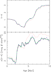
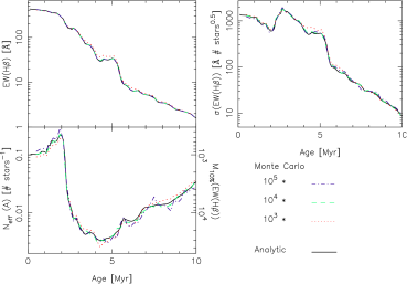
Figure 9: Comparison with Monte Carlo simulations: Left Panel: V–K color index Top left: Evolution of the V–K color index for the analytical and Monte Carlo simulations. Bottom left: Comparison of the normalised value of $\sigma$(V–K) for the analytical and Monte Carlo simulations. Middle and Right Panels: EW(H$\beta$). Top middle: Evolution of EW(H$\beta$) for the analytical and Monte Carlo simulations. Bottom middle: Normalised $N_{\mathrm{eff}}$(EW(H$\beta$)) for the analytical and Monte Carlo simulations. Top Right: Comparison of the normalised value of $\sigma$(EW(H$\beta$)) for the analytical and Monte Carlo simulations.

The top left panel of Fig. 9 shows the comparison of the mean V–K colour index for the different simulations and the analytical solution. The values are clearly consistent with each other, and show not only that the analytical formalism is a very good approximation, but also that the formalism can be used in place of Monte Carlo simulations.

There are, however, some deviations in the 10³ stars cluster simulations. As shown in Cerviño and Mas-Hesse (1994) the V–K colours at the ages where the major discrepancies appear are mostly dominated by the presence of RSGs. The differences between the analytical estimation of the dispersion and the real one (as obtained from Monte Carlo runs)is perhaps due to the low number of stars responsible of the colours. For such a small number of stars the sampling is too poor to be meaningful. In these low mass clusters the analytical dispersion provides only a first order approximation to the real one, that can only be obtained from Monte Carlo simulations. The lower left panel shows the comparison of the normalised values of $\sigma_{\mathrm{clus}}$(V–K) with the analytical value. It shows that the analytical dispersion and the Monte Carlo results are very similar.

We also show in Fig. 9 the 90% confidence levels of the different simulations. It is important to highlight that these confidence level bands are not symmetric with respect to the mean value.

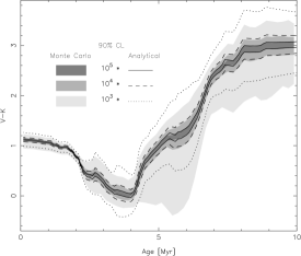
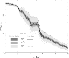
Figure 10: Comparison of analytical confidence levels with Monte Carlo simulations. Left Panel: V–K colour index. Right Panel: EW(H$\beta$)

.

It is also possible to obtain confidence level bands analytically, as shown in Fig. 10. The analytical confidence levels have been obtained using the approximations found by Gehrels (1986) for Poisson statistics. We have used the corresponding denormalised $N_{\mathrm{eff}}$, (i.e. $N_{\mathrm{eff}}^{*}$) for the EW(H$\beta$) and the $\mathrm{L}_{\mathrm{V}}/\mathrm{L}_{\mathrm{K}}$ observables as the Poisson parameter. The resulting confidence levels have been multiplied by $A/N_{\mathrm{eff}}^{*}$ with $A$ corresponding to EW(H$\beta$) or $\mathrm{L}_{\mathrm{V}}/\mathrm{L}_{\mathrm{K}}$. In the case of V–K, the resulting confidence level of $\mathrm{L}_{\mathrm{V}}/\mathrm{L}_{\mathrm{K}}$ has been transformed into the corresponding V–K value.

The analytical estimation of confidence levels for clusters with masses larger than 10³ stars provides a very good approximation to the one obtained in the Monte Carlo simulations, showing, a posteriori, that the actual probability distribution function is well approximated by a Poisson distribution.

5 Discussion and conclusions

In this paper we have reviewed the effects of sampling fluctuations in evolutionary synthesis codes. We have presented an approximate, and yet accurate, analytical formalism which allows the estimation of Poisson dispersions for any observable synthetised by population codes. It is important to take into account that these dispersions vary from observable to observable and cannot be extrapolated. We provide some simple cases (Appendix A) for a variety of observables. The comparison of these analytical dispersions with proper Monte Carlo simulations shows that the formalism is valid, and hence bypasses the need to perform Monte Carlo simulations to evaluate the dispersion in any given observable. The formalism is simple enough that it can (and must) be implemented in all the synthesis codes to assess the predicted dispersions in the computed observables. We also stress the importance of evaluating the covariance terms when estimating the Poissonian dispersion.

As an illustrative example of the formalism, we have implemented it for the case of young starbursting clusters. We find that in general the UV observables are the best defined ones (i.e. they have the lowest Poissonian dispersions). The less reliable continuum range corresponds to the hard ionising flux. In particular, a relative dispersion smaller than 10% for the hard ionising flux can only be achieved for clusters more massive than 5 10⁴ M_⊙. The situation becomes even worse when WR stars appear in the cluster. In that case a mass of about 10⁶ M_⊙ is needed to ensure an uncertainty of about 10%. The implications of such effects on the use of evolutionary synthesis models as input for photoionisation ones remain to be evaluated.

In the case of WR stars, we have shown that the most reliable observable for the determination of the WR population is the ratio between the WR bump at 4686 Å and the H$\beta$ luminosities. We have also shown that the presence of WR stars is a quite poorly-defined property of star forming regions, due to small number statistics. In particular, it is possible that the general failure of synthesis models to predict the WR population in our Galaxy could be solved taking into account the dispersion in real clusters due to Poissonian fluctuations in addition to the dispersion introduced by the star formation history.

We have also shown that the dispersions and confidence levels derived analytically are in good agreement with the dispersions obtained from Monte Carlo simulations for clusters containing more than 10³ stars, i.e. more than $5\times 10^{3}$ M_⊙ transformed into stars in the mass range 2 – 120 M_⊙ following a Salpeter IMF. The confidence levels and dispersions obtained can be used as a first order evaluation of the number of Monte Carlo simulations needed to obtain reliable results, or used directly in the comparison with observed data.

Appendix A Observables, error propagation and the effective number of stars $N_{\mathrm{eff}}$

To illustrate the use of the $N_{\mathrm{eff}}$  formalism for a variety of astrophysical observables, we give here a few examples to help the reader. For a complete review on error propagation, see Kendall & Stuart (1977) or a simplified version by Leo (1992) and its adaptation on the NED server at http://nedwww.ipac.caltech.edu/level5.

Let us assume a random variable $u$ which is a function of two random variables $u=f(x,y)$. Let us also assume that $\sigma_{x}^{2}$ and $\sigma_{y}^{2}$ are the variances of these variables. The variance of the random variable $u$, $\sigma_{u}^{2}$, can be approximated as

$$\sigma_{u}^{2}\simeq\left(\frac{\partial f}{\partial x}\right)^{2}\sigma_{x}^{2}+\left(\frac{\partial f}{\partial y}\right)^{2}\sigma_{y}^{2}+2{\mathrm{cov}}(x,y)\frac{\partial f}{\partial x}\frac{\partial f}{\partial y}$$ (17)

where ${\mathrm{cov}}(x,y)$ is the covariance. This equation is exact if the function $f$ is linear in the $x$ and $y$ variables. The covariance can be related to the linear correlation coefficient, $\rho(x,y)$, defined as

$$\rho(x,y)=\frac{{\mathrm{cov}}(x,y)}{\sigma_{x}\sigma_{y}}$$ (18)

The correlation coefficient varies between $-1$ and $+1$ where the sign indicates the sense of the correlation.

We can give a more general definition of the effective number of stars $N_{\mathrm{eff}}$, as introduced by Buzzoni (1989), to any observable. As it was pointed out in Sect. 2, we can define a $N_{\mathrm{eff}}(A)$ of any synthesized quantity $A$ which is the sum of the contributions from individual stars (or populations), $A=\sum\omega_{i}a_{i}$, and thus it has a variance $\mathrm{var}(A)=\sum\mathrm{var}(\omega_{i})a_{i}^{2}$ (c.f. Eq. 20). The relative error is then

$$\frac{\mathrm{var}(A)^{1/2}}{A}=\frac{\left(\sum\omega_{i}a_{i}^{2}\right)^{1/2}}{\sum\omega_{i}a_{i}}=\frac{1}{\sqrt{N_{\mathrm{eff}}(A)}}$$ (19)

Note that if $A$ is normalised to the total mass, $N_{\mathrm{eff}}(A)$ is also normalised. So $N_{\mathrm{eff}}(A)$ gives an estimate of the relative error (and hence, of the absolute error) for any possible value of the mass transformed into stars.

A.1 Error in the multiplication by a constant

Let us assume an observable random variable $u(x)=a\,x$ where $a$ is a constant. with Eq. 17 one obtains

$$\sigma_{u}^{2}=a^{2}\,\sigma_{x}^{2}$$ (20)

and the relative error

$$\frac{\sigma_{u}}{u}=\frac{\sigma_{x}}{x}=\frac{1}{\sqrt{N_{\mathrm{eff}}(x)}}=\frac{1}{\sqrt{N_{\mathrm{eff}}(u)}}$$ (21)

This is the more general case used in synthesis codes, as it is showed in Eq. 14.

A.2 Error of a sum

Let us now assume an observable random variable $u=x+y$. In this case

$$\sigma_{u}^{2}=\sigma_{x}^{2}+\sigma_{y}^{2}+2{\mathrm{cov}}(x,y)$$ (22)

The value of ${\mathrm{cov}}(x,y)$ depends on the observables we use, as shown by Eq. 14.

An interesting case comes from the computation of the luminosity in a band, for example $L_{\mathrm{B}}$, obtained by the integration of the monochromatic flux, $f(\lambda)$, over the filter response of the band, $R(\lambda)$:

$${\mathrm{L}}_{\mathrm{B}}=\int{f(\lambda)*R(\lambda)\;{\mathrm{d}}\lambda}\simeq\sum_{i}f(\lambda_{i})\,R_{\lambda_{i}}\,\Delta\lambda_{i}$$ (23)

where we have approximated the value of the integral by the resulting value from the use of the trapezium rule and the individual monochromatic fluxes, $f(\lambda_{i})$ and band transmission coefficients, $R_{\lambda_{i}}$. The corresponding variance due only to the error in the monochromatic luminosities, $\sigma_{f(\lambda_{i})}=\sigma_{i}$, can be obtained from Eq. 17 and using Eq. 21 and Eq. 22:

$$\sigma_{{\mathrm{L}}_{\mathrm{B}}}^{2} = \sum_{i}\left[R_{\lambda_{i}}\,\Delta\lambda_{i}\right]^{2}\sigma_{i}^{2}\$$ (24)

$$+\sum_{i<j}2\,{\mathrm{cov}}\left(f(\lambda_{i}),f(\lambda_{j})\right)\,R_{\lambda_{i}}R_{\lambda_{j}}\,\Delta\lambda_{i}\Delta\lambda_{j}$$

Note also that the resulting variance (and corresponding $N_{\mathrm{eff}}$) must be similar to the one obtained if the synthesis code computes ${\mathrm{L}}_{\mathrm{B}}$, summing up the individual ${\mathrm{L}}_{{\mathrm{B}}_{i}}$ and using Eq. 19.

A.3 Error of a difference

Let us assume an observable random variable $u=x-y$. The corresponding variance is

$$\sigma_{u}^{2}=\sigma_{x}^{2}+\sigma_{y}^{2}-2{\mathrm{cov}}(x,y)$$ (25)

A typical example in synthesis codes is the computation of colour indexes. As an example, for the U-B colour index one obtains (see also below for the error of a logarithm):

$$\sigma_{\mathrm{U-B}}^{2}=\sigma_{\mathrm{U}}^{2}+\sigma_{\mathrm{B}}^{2}-2{\mathrm{cov(U,B)}}$$ (26)

This leads to $\sigma_{\mathrm{U-B}}^{2}\simeq(\sigma_{\mathrm{U}}-\sigma_{\mathrm{B}})^{2}$ if the correlation coefficient is 1, as it is assumed by Buzzoni (1993) and Lançon and Mouhcine (2000) for colours where the corresponding fluxes originate from the same population (but it is not the general case for integrated colours from different stellar populations). Note that the error in colour indices may be lower than the error in the corresponding colours, depending on the covariance term.

A.4 Error of a product

Let us assume an observable random variable $u=x\,y$. In this case

$$\sigma_{u}^{2}=x^{2}\sigma_{y}^{2}+y^{2}\sigma_{x}^{2}+2\,x\,y\,{\mathrm{cov}}(x,y)$$ (27)

so that

$$\frac{\sigma_{u}^{2}}{u^{2}}=\frac{\sigma_{x}^{2}}{x^{2}}+\frac{\sigma_{y}^{2}}{y^{2}}+2\frac{{\mathrm{cov}}(x,y)}{x\,y}$$ (28)

We can rewrite the relative error as a function of $N_{\mathrm{eff}}$. When the correlation coefficient is zero (cov($x,y$)=0) :

$$\frac{\sigma_{u}^{2}}{u^{2}}=\frac{1}{N_{\mathrm{eff}}(u)}\simeq\frac{1}{N_{\mathrm{eff}}(x)}+\frac{1}{N_{\mathrm{eff}}(y)}$$ (29)

while if the correlation coefficient is 1, cov($x,y$)=$\sigma_{x}\sigma_{y}$ and

$$\frac{\sigma_{u}^{2}}{u^{2}}=\frac{1}{N_{\mathrm{eff}}(u)}\simeq\left(\frac{1}{\sqrt{N_{\mathrm{eff}}(x)}}+\frac{1}{\sqrt{N_{\mathrm{eff}}(y)}}\right)^{2}$$ (30)

In the general case:

$$\frac{\sigma_{u}^{2}}{u^{2}} = \frac{1}{N_{\mathrm{eff}}(u)}$$ (31)

$$\simeq \frac{1}{N_{\mathrm{eff}}(x)}+\frac{1}{N_{\mathrm{eff}}(y)}+2\frac{{\mathrm{cov}}(x,y)}{x\,y}$$

This is the case, for example, of the computation of the dispersion in the mechanical energy or mechanical power as given by the mass-loss of the stars in the cluster and their terminal velocities.

A.5 Error in a ratio

Let us assume an observable random variable $u=x/y$ where $y$ is non zero. The resulting equation for the relative error is

$$\frac{\sigma_{u}^{2}}{u^{2}}\simeq\frac{\sigma_{x}^{2}}{x^{2}}+\frac{\sigma_{y}^{2}}{y^{2}}-2\frac{{\mathrm{cov}}(x,y)}{x\,y}$$ (32)

which is similar to Eq. 28 but changing the sign which corresponds to the covariance term.

In this case the normalisation is very important. Since the normalised quantity is $\sigma^{2}$, then $x^{2}/\sigma_{x}^{2}$, $y^{2}/\sigma_{y}^{2}$ and $x\,y/\mathrm{cov}(x,y)$ have the same normalisation as $x$ or $y$, and so is $u^{2}/\sigma_{u}^{2}$ which has the same normalisation as $x$ or $y$. And since $u$ is dimensionless $1/\sigma_{u}^{2}$ is the normalised quantity (and not $\sigma_{u}^{2}$ as in the general case). Note that the larger the mass of the cluster the larger should the absolute error be, which makes no sense. It also shows the advantage of using $N_{\mathrm{eff}}$ instead of $\sigma^{2}$ for the description of errors: $N_{\mathrm{eff}}$ always keeps the same normalisation.

Ratios are used a lot in synthesis codes (equivalent widths, populations ratios, fractional contributions, etc.) so let us illustrate some particular cases.

1. $y=x+z$ where ${\mathrm{cov}}(x,z)=0$. This case is illustrative for population ratios, say the WC/WR ratio. The resulting relative error as a function of $x,y$ is:

   $$\frac{\sigma_{u}^{2}}{u^{2}}\simeq\frac{\sigma_{x}^{2}}{x^{2}}+\frac{\sigma_{y}^{2}}{y^{2}}-2\frac{\sigma_{x}^{2}}{x\,y}$$ (33)

   For the particular case of ratios of population numbers it is easy to show that $\sigma_{x}^{2}=x=N_{\mathrm{eff}}(x)$ and thus

   $$\frac{\sigma_{u}^{2}}{u^{2}}=\frac{1}{N_{\mathrm{eff}}(u)}\simeq\left|\frac{1}{N_{\mathrm{eff}}(x)}-\frac{1}{N_{\mathrm{eff}}(y)}\right|$$ (34)

2. $y=r+z$ where cov$(r,z)=0$, but cov$(r,x)\neq 0$: This case is illustrative for ratios of line luminosities, say the L(WRbump)/L(H$\beta$) ratio, where the WR has a contribution to L(H$\beta$). The resulting relative error is

   $$\frac{\sigma_{u}^{2}}{u^{2}}\simeq\frac{\sigma_{x}^{2}}{x^{2}}+\frac{\sigma_{y}^{2}}{y^{2}}-2\frac{{\mathrm{cov}}(r,x)}{x\,y}$$ (35)

   In this case, we need to know the value of ${\mathrm{cov}}(r,x)$, say the contribution of WR stars to the H$\beta$ luminosity, in order to evaluate the error.

3. $y=r+z$ where cov$(r,z)\neq 0$, but cov$(r,x)\neq 0$: This case is illustrative for ratios of equivalent widths, where, for example, $x$ is the L(H$\beta$), $r$ is the nebular continuum and $z$ the stellar one. The resulting relative error is

   $$\frac{\sigma_{u}^{2}}{u^{2}} \simeq \frac{\sigma_{x}^{2}}{x^{2}}+\frac{\sigma_{r}^{2}+\sigma_{z}+2\,{\mathrm{cov}}(r,z)}{y^{2}}$$ (36)

   $$-2\frac{{\mathrm{cov}}(x,r)+{\mathrm{cov}}(x,z)}{x\,y}$$

   which becomes Eq. 32. In the study of covariance terms, it is not necessary to worry about which are the contributions if the covariance terms have been properly taken into account.

A.6 Error in a logarithm

Last, but not least, let us assume that $u=a\log x$ + c, where $a$ and $c$ are constants. Using Eq. 17:

$$\sigma_{u}^{2}=a^{2}\,\frac{\sigma_{x}^{2}}{x^{2}}=\frac{a^{2}}{N_{\mathrm{eff}}(x)}$$ (37)

The denormalised value of the effective number of, say, $N_{\mathrm{eff}}({\mathrm{B}})$, where B is the Johnson B band, gives us the absolute error in the B magnitude for the given mass transformed into stars.

For the case of colours indices, say U-B, using the Eq. 26

$$\sigma_{\mathrm{U-B}}^{2} \simeq (2.5\times\log_{10}(e))^{2}\left[\frac{1}{N_{\mathrm{eff}}({\mathrm{L}}_{\mathrm{U}})}+\frac{1}{N_{\mathrm{eff}}({\mathrm{L}}_{\mathrm{B}})}\right.$$ (38)

$$\left.-2\frac{\mathrm{cov}({\mathrm{L}}_{\mathrm{U}},{\mathrm{L}}_{\mathrm{B}})}{{\mathrm{L}}_{\mathrm{U}}\,{\mathrm{L}}_{\mathrm{B}}}\right]$$

Note that a $N_{\mathrm{eff}}$(U-V) value cannot be obtained due to the logarithm dependence in the luminosities. This situation is general for all the colors indices.

References

- Barbaro & Bertelli (1977) Barbaro, C. & Bertelli, C. 1977, A&A, 54, 243
- Brocato et al. (1999) Brocato, E., Castellani, V., Raimondo, G., & Romaniello, M. 1999, A&AS, 136, 65
- Bruzual (2001) Bruzual, G. 2001 in The Evolution of Galaxies. I-Observational Clues, Kluwer Academic Publishers, J.M. Vilchez, G. Stasińska and E. Pérez (eds.) in press
-
Buzzoni (1989)
Buzzoni, A. 1989, ApJS, 71, 871
http://www.merate.mi.astro.it/eps/home.html - Buzzoni (1993) Buzzoni, A. 1993, A&A, 275, 433
- Cerviño and Mas-Hesse (1994) Cerviño, M. & Mas-Hesse, J.M. 1994, A&A, 284, 749
- Cerviño et al. (2000) Cerviño, M., Luridiana, V. & Castander, F.J. 2000, A&A, 360, L5
- Cerviño et al. (2001a) Cerviño, M., Mas-Hesse, J.M. & Kunth, D. 2001a, A&A, (submitted)
- Cerviño et al. (2001b) Cerviño, M., Gómez-Flechoso, M.A., Castander, Schaerer, D., F.J., Mollá, M., Knödlseder, J., & Luridiana, V. 2001b, A&A, 2001. 376, 422
- Chiosi, Bertelli & Bressan (1998) Chiosi, C., Bertelli, G., & Bressan, A. 1998, A&A, 196, 84
- Gehrels (1986) Gehrels, N. 1986, ApJ, 303, 346
- Girardi & Bica (1993) Girardi, L. & Bica, E. 1993 A&A, 274, 279
- Kendall & Stuart (1977) Kendall M., Stuart A. 1977, The advanced theory of statistics, Volume 1 (London: Griffin)