Modeling the corona of AB Doradus

G.A.J. Hussain¹, A.A. van Ballegooijen¹, M. Jardine², A. Collier Cameron²

Abstract

We present a model for the coronal topology of the active, rapidly rotating K0 dwarf, AB Doradus. Surface magnetic field maps obtained using a technique based on Zeeman Doppler imaging indicate the presence of a strong non-potential component near the pole of the star. The coronal topology is obtained by extrapolating these surface maps. The temperature and density in the corona are evaluated using an energy balance model. Emission measure distributions computed using our models compare favorably with observations. However, the density observed by EUVE, $n_{e}\approx 10^{13}$ cm^-3, at the emission measure peak temperature of $8\times 10^{6}$ K remains difficult to explain satisfactorily.

¹¹footnotetext: Harvard Smithsonian CfA²²footnotetext: University of St Andrews

1. Introduction

AB Doradus is a well studied example of the class of very active, rapidly rotating cool stars that are just evolving onto the main sequence. Its youth is indicated by strong lithium absorption and it rotates at 50 times the solar rate (P_rot=0.51d). AB Dor’s rapid rotation makes it an ideal candidate for high resolution spectroscopic techniques such as Doppler imaging. Surface maps obtained using this technique since 1992 typically show the presence of a dark polar spot region which extends down to about 70^∘ latitude, co-existing with lower latitude spots near the equator. Spots are recovered to within the resolution capability of the techniques so it is likely that smaller spot features also exist at the surface that cannot be resolved. Photometry of the star from 1978 indicates that AB Dor may follow a solar-type activity cycle spanning 22-23 years (Amado et al. 2001).

The locations of the lower-latitude spots change from year-to-year and are believed to have lifetimes of about a month. The polar spot is much more long-lived, as it has been recovered in every spot map obtained of AB Dor except for the first, where there there is no evidence of a polar spot (Kürster et al. 1997). This early image was derived using data taken in 1988 and its epoch coincides with a maximum in spot activity according to the star’s photometric light level. Hence the polar spot may be tied in with the stellar activity cycle. The presence of the polar cap does indicate that a considerable quantity of flux is emerging at the pole of the star. This polar spot “phenomenon” is common to spot maps recovered on other rapidly rotating systems ranging from RSCVn binaries to young G dwarfs (Vogt & Penrod 1983, Strassmeier 1990, Barnes et al. 1998).

Refer to caption — Figure 1.: Emission measure distribution from 1993-1994 for AB Dor computed from IUE and EUVE data (Sanz-Forcada et al. this volume).

Coronal activity indicators in the X-ray, radio and optical wavelengths suggest strong variability in the stellar corona. However, while it is clear that AB Dor emits strongly in X-rays, L_x/L ${}_{bol}\approx 10^{-3}$ (Vilhu & Linsky 1987) the characteristics of the emitting structures have yet to be ascertained.

Observations of the stellar corona obtained from a variety of sources indicate the presence of both extended and compact structures. The evidence for extended coronal features, with sizes of over a stellar radius can be inferred from several sources. Large prominence type complexes are detected through fast-moving absorption transients moving through the hydrogen Balmer lines. These slingshot prominences are supported at distances of between 2-5 $\mbox{R}_{*}$ and hence well above the Keplerian corotation radius of the star ( $R_{k}\approx$ 2.6 $\mbox{R}_{*}$ ) (Donati et al. 1999). The prominence lifetimes are not known but typically have upper limits of about 2 rotation periods (i.e. 1 day). There is further evidence for extended structures from FUSE and HST datasets. These reveal transition region lines (C iv 1548Å, Si iv 1393Å, O vi 1032Å) with broadened wings in emission extending to velocities of 270km/s. These wings are caused by optically thin plasma ( $T\approx 10^{5}$ K) at heights out to the co-rotation radius, 2.6 $\mbox{R}_{*}$ (Brandt et al. 2001, Young 2001).

Evidence for compact coronal features comes from flare decay analysis on lightcurves obtained using BEPPOSAX (Maggio et al. 2000). They find that the flaring region is small ( $H<0.3$ $\mbox{R}_{*}$ ) and that it is uneclipsed over a full rotation cycle, indicating that it is located near the pole of the star. A statistical analysis of ROSAT data spanning a period of 5 years suggests rotational modulation at 5-13% (Kürster et al. 1997). Brandt et al. (2001) find that between 60% to 80% of the emission should originate near the stellar photosphere.

Measurements of pressure in the corona are extremely high, over two orders of magnitude larger than those found on the quiet Sun. Using HST and Chandra data, electron densities are found to be high, $n_{e}\approx 2-3\times 10^{12}$ cm^-3, at transition region temperatures (about $3\times 10^{4}$ K) (Brandt et al. 2001, Linsky 2001). At higher temperatures, around $3\times 10^{6}$ K, recent XMM results indicate electron densities of $n_{e}\approx 3\times 10^{10}$ cm^-3 (Güdel et al. 2001). Sanz-Forcada et al. (this volume) compute an emission measure distribution (EMD) for AB Dor by combining IUE and EUVE observations taken in 1993 and 1994. The resulting EM is shown in Fig. 1. C ii, iii, iv, v lines from the IUE dataset have been used to constrain emission measures under $\approx 10^{5}$ K while Fe xix, xx, xxi, xxii lines from the EUVE dataset have been used to evaluate the emission measure at higher temperatures. Density sensitive lines observed by EUVE indicate extremely high densities ( $10^{12}<n_{e}<10^{13}$ cm^-3) at temperatures between $6-8\times 10^{6}$ K. Sanz-Forcada et al. (this volume) speculate that this EM peak is caused by compact structures with strong magnetic fields that are capable of supporting this kind of high-pressure gas. Results from similar rapidly rotating systems indicate that this peak is very stable. Brickhouse & Dupree (1998) suggest that an analogous EM peak observed in the EUVE EMD of the contact binary, 44i Boo, can be explained in terms of loops with heights of about 0.004 $\mbox{R}_{*}$ . We set out to explain the observations outlined in this section using simple models based on extrapolations of AB Dor’s surface magnetic field. We use magnetic field maps obtained using the high resolution spectroscopic technique of Zeeman Doppler imaging.

2. Advanced ZDI

Zeeman Doppler imaging (ZDI) is essentially Doppler imaging applied to circularly polarized spectra (Semel 1989). As with Doppler imaging, ZDI relies on rotational broadening to separate the signatures from different magnetic field regions on the surface in velocity-space. Circularly polarized spectra are sensitive to the line-of-sight component of the magnetic field. Within the weak field regime (under 1kG) the size of the signature scales linearly with the size of the field. By tracking the velocity excursions and intensity variations of the circularly signatures over the course of a rotation cycle we can determine the orientation as well as the size of the surface field (Donati & Brown 1997). Magnetic field maps of AB Dor obtained using this technique typically show strong azimuthal field at the pole of the star. This very non-solar pattern is puzzling and doubts have been cast over its authenticity, partly due to uncertainties introduced in the conventional ZDI method. Some uncertainties are due to the assumption that all field orientations (radial, azimuthal and meridional fields) are assumed to be independent of each other. This means that it is possible to reconstruct monopoles at the stellar surface and equally physically unrealistic fields.

Hussain et al. (2001) describe an advanced version of ZDI that introduces a relationship between different field orientations by assuming a potential field. As well as assuming a relationship between radial, azimuthal and meridional field vectors these maps can also be used to extrapolate out to the stellar corona. The technique we present here is more advanced as it incorporates departures from potential field distributions. While this solution is not force-free it allows us to pinpoint the areas where the surface field distribution becomes non-potential while still allowing for the extrapolation of the field out to the corona.

2.1. Doppler maps

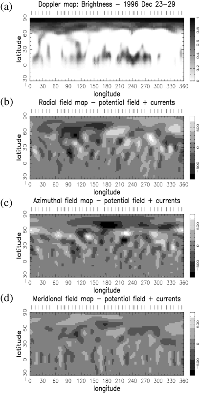
The dataset used to obtain the maps shown in Fig. 2 was obtained using the 3.9m Anglo-Australian telescope, UCL Echelle spectrograph and the Semel polarimeter in 1996 December 23-29. Data were reduced using the dedicated echelle reduction software package, esprit (Donati et al. 1997). Once reduced, the signal from over 1500 photospheric lines were “summed up” using a technique called least squares deconvolution. This technique allows us to increase signal-to-noise levels by a factor of 30. Full details on the instrument setup, data reduction and deconvolution can be found in previous papers (Donati et al. 1999, Hussain et al. 2000).

Data were combined from all four nights (1996 Dec. 23, 25, 27 and 29) in order to obtain as complete phase coverage as possible. The surface differential rotation rate as measured by Donati & Collier Cameron (1997) has been incorporated into the code to account for the shear of surface features over the course of a week. The brightness map was produced using the Doppler imaging code, dots (Collier Cameron 1997), and the magnetic field maps shown here are produced using the code described above. We tried initially to fit the observed circularly polarized spectra using just a potential field distribution. However, it was not possible to find a solution within a reduced $\chi^{2}\approx 1.5$ for this dataset. We then tried a model in which the curl of the magnetic field $\mbox{ \bf j}=\nabla\times\mbox{\bf B}$ is given by a potential field ( $\mbox{\bf j}=-\nabla\Psi$ , with $\nabla^{2}\Psi=0$ ). The magnetic field is determined by two free functions, $B_{r}(\theta,\phi)$ and $j_{r}(\theta,\phi)$ , at the stellar surface. This provides the additional freedom to obtain a good fit to the polarization profiles and also allows the magnetic field to be extrapolated into the corona in a realistic way. The brightness and magnetic field maps are produced independently of each other and are shown in Fig. 2.

We find that the non-potential part of the magnetic field is found mostly in the strong azimuthal field band above about 70^∘ latitude. This non-potential region is located around the boundary of the dark polar spot that is recovered using Doppler imaging (c.f. Figs. 2a & c). The magnetic field distribution recovered using this method agrees with the maps obtained previously using conventional ZDI (Donati et al. 1999). The main differences between the ZD maps and these images are in the azimuthal maps; specifically in the unbroken band of uni-directional flux. While there is still a strong clockwise azimuthal component near the pole in this model, it is weaker than that found in the Zeeman Doppler map and is even broken by a region of opposite polarity. The strong azimuthal field pattern is clearly non-solar. On the Sun, horizontal field is largely confined to the penumbrae of starspots and would cover a relatively small area.

Several points must be kept in mind when interpreting the images in Fig. 2. The magnetic field analysis assumes that the spectral line depth is uniform over the stellar surface and does not take the presence of dark starspots into account. It is likely that the actual field in the starspots is much stronger than that reconstructed using ZDI. In particular, as the brightness and line depth in the polar region are suppressed, the field from this region will not contribute to the circularly polarized spectra. It is possible that there is very strong radial field in the center of the polar spot and that all we can observe using the circularly polarized profiles is the brighter penumbral region. Another point to keep in mind is that the meridional (N-S) component has a reduced contribution to circularly polarized spectra obtained from high inclination stars like AB Dor ( $i=60^{\circ}$ ). This explains why the field recovered in Fig. 2d is weak compared to the radial and azimuthal field maps.

2.2. Coronal extrapolation of the surface field

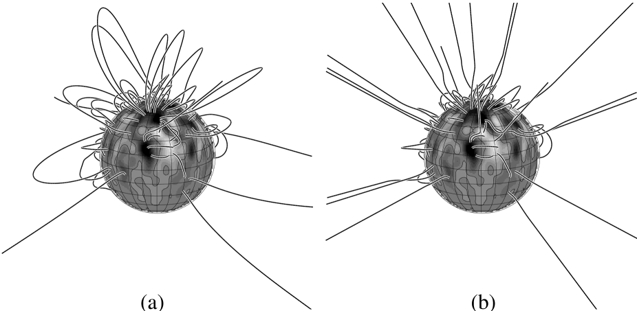
The magnetic field, B, can be written in terms of spherical harmonic functions, and the assumption that, $\mbox{\bf j}=-\nabla\Psi$ can be used to determine the radial dependence of the spherical harmonic coefficients. The resulting field pattern is shown in Fig. 3. As prominences are observed out to 5 $\mbox{R}_{*}$ we initially computed the field topology by setting the source surface to 5 $\mbox{R}_{*}$ (Fig. 3a). The source surface is the point beyond which all the field is assumed to be open. The technique developed by Jardine et al. (2001) allows us to evaluate locations around AB Dor that can support slingshot prominences. Applying this technique to this model shows that the field around AB Dor is complex enough to support prominences at sufficiently large distances around AB Dor, if the source surface radius is set to values above 5 $\mbox{R}_{*}$ . Fig. 3b shows the field topology for the same model but with the source surface set to 1.6 $\mbox{R}_{*}$ , which is the value suggested by our modeling of coronal loops (see below). If this is the case it is unclear how prominences can be supported.

3. Heating in stellar corona

We have used the 3D magnetic field models shown in Figs. 3a & b to study coronal heating in AB Dor. In our model we take non-thermal heating to be constant in time and seek steady state solutions of the energy balance equations. As the loops are allowed to be asymmetric, there is in general a steady mass flow along the loop. The flow velocity is assumed to be smaller than the sound speed, so the plasma is nearly in hydrostatic equilibrium. We assume that magnetic flux is constant along the loop. Hence, as the magnetic field strength, $|B|$ , drops off with height, the loop cross-sectional area will expand (Schrijver et al. 1989). Energy transport in the lower transition region ( $T<4\times 10^{5}$ K) is modeled using a parametrization of ambipolar diffusion. Boundary conditions placed on the footpoints of each loop include setting the footpoint temperature to $T=2\times 10^{4}$ K, and energy fluxes are calculated for each footpoint assuming a simple model of the chromosphere.

The heating rate is assumed to depend only on the magnetic field strength:

E_{H}(s)=\epsilon_{0}B(s)^{n},

(1)

where $E_{H}$ is the heating rate per unit volume as function of position, $s$ , along the loop, and $\epsilon_{0}$ is a constant. We find that, if the heating rate is proportional to $B$ ( $n=1$ ), then for high-altitude loops $E_{H}$ drops off quickly with height and there is insufficient heating at the apex of the loops for a stable solution. Thermal instabilities arise because the heating at the footpoints is strong, increasing pressure everywhere in the loop. The heating rate cannot compensate for local radiative losses at the top of the loop and this triggers the formation of a cool coronal condensation. Therefore, in the present paper we focus on models with heating independent of field strength, $n=0$ .

In this paper we assume that the EMD peak is caused by loops with a maximum temperature $T_{max}\approx 8\times 10^{6}$ K. Therefore the constant, $\epsilon_{0}$ , is selected to fit $T_{max}$ , so for short loops $\epsilon_{0}$ must be very large, and for long loops $\epsilon_{0}$ must be very small. The resulting gas pressure is inversely proportional to loop length, L. We find that for high-altitude loops the gas pressure is larger than the magnetic pressure at the apex of the loop, i.e. the coronal plasma is no longer magnetically contained. This problem arises for loop heights greater than about 0.6 $\mbox{R}_{*}$ , which suggests that beyond this height all magnetic fields are open. Therefore, in the following we only present results for the model with the source surface at 1.6 $\mbox{R}_{*}$ (see Fig. 3b).

To obtain a clear peak in the EMD it is necessary to assume that the cross-section varies with position along the loop. By allowing a loop to expand with height, emission at lower temperatures is suppressed as the legs of the loops at these temperatures have a smaller cross-section. The hotter gas at the loop apex fills a larger volume and produces the type of emission peak that is observed (Schrijver et al. 1989, Ciaravella et al. 1996). Expansion factors ( $\Gamma=A_{max}/A_{foot}$ ) of between 5-7 are sufficient to explain the enhanced peak observed in Fig. 1.

First, we investigate the type of compact loops that are thought to be the source of high density measurements at EM peak temperatures (Sanz-Forcada et al. 2001, Brickhouse & Dupree 1998). We find that, in order to obtain stable loops with coronal density of about $10^{13}$ cm^-3 as observed by EUVE, we have to increase the heating rate such that $\epsilon_{0}\approx 4\times 10^{3}$ erg cm^-3 s^-1 and we have to reduce the loop length to $L\approx 280$ km (we assume $\Gamma=6$ ). The gas pressure in such loops would be about $10^{4}$ dyne/cm² and the field strength at the feet of such loops must be at least 3000 G, which is larger than the fields observed with ZDI. Assuming there are about $10^{4}$ such loops at any one time, we can fit both the observed EMD (see Fig. 4a) and the densities at the EM peak. However, their lengths are unrealistic as they are comparable with the height of the photosphere. Furthermore it is unclear why such short loops would have expanding cross-sections, $\Gamma>5$ .

Another more realistic model can reproduce the observed EMD but is inadequate when explaining the high densities in the EM peak. As mentioned earlier, expansion factors of $5<\Gamma<7$ are needed to reproduce the EM peak in Fig. 1. These factors can be obtained using the model shown in Fig. 3b and assuming loop heights in the range 0.1-0.5 $\mbox{R}_{*}$ . The average length of such a loop is about 0.75 $\mbox{R}_{*}$ and if $\epsilon_{0}\approx 10^{-3}$ erg cm^-3 s^-1, it will have a pressure of about $5$ dyne/cm², consistent with the TR observations. However, the loops have coronal densities of $\approx 3\times 10^{9}$ cm^-3 at $T\approx 8\times 10^{6}$ K, much less than implied by the EUVE observations. In order to produce higher densities, it is possible to invoke much smaller loops ( $L\approx 0.043$ $\mbox{R}_{*}$ ) with high heating rates and small expansion factors to fit the high temperature tail. The EM resulting from a combination of these two types of loops is plotted in Fig. 4b. These hot loops have densities of $n_{e}\approx 10^{13}$ cm^-3 at the EM peak temperature, but they contribute only 3% of the emission at this temperature. Therefore, it is unlikely that this model can reproduce the observed density sensitive lines.

Both models presented here fit the observed EMD well. The model that can reproduce the observed densities as well as fit the EM requires loops that are too short (on the same scale as the height of the photosphere). The second model would appear more reasonable but it cannot reproduce the observed density sensitive lines. Therefore, neither model is fully satisfactory.

4. Discussion

Magnetic field maps of AB Dor from 1996 December show very strong azimuthal field. The non-potential part of the field distribution is concentrated around the boundary of the dark stable polar spot that extends down to about 70^∘ latitude. This azimuthal field has no solar analogy but as it is likely that the polar cap is censoring the field at the pole of the star these maps may not present the full picture. If strong radial field is concentrated in the most spotted parts of the star, we may only be detecting the penumbral regions of the spots located at the pole. Schrijver (this volume) describes a model for a spun-up solar-type star. According to this model there are three bands of alternating polarity encircling the pole. If the star is rotating rapidly, the field lines connecting between the different bands are likely to be sheared in one direction, thus producing a strong unidirectional azimuthal field near the pole. However, we find no evidence for bands of alternating polarity near the pole in our ZDI maps. If they exist, the polarization signature from the alternating radial field bands is buried in the dark polar spot and hence cannot be detected using our method of magnetic field mapping.

By extrapolating our surface maps, we can model the coronal topology of the star. These coronal fields can then be used to model heating as well as to evaluate sites of stable mechanical equilibria that can support slingshot-type prominences. The fields are sufficiently complex to support prominences out to the distances at which they are observed (2-5 $\mbox{R}_{*}$ ) assuming the source surface is extending out this far. It may be necessary to compensate for the missing flux at the pole and model for the flux we cannot observe in the unseen hemisphere of AB Dor (stellar inclination=60^∘). By adding this missing flux it is likely that the global pattern will be modified from the type presented here and that it will become dominated by a dipole field (Jardine et al. 2001).

Using heating rates that can reproduce the observed transition region densities and pressures, we can fit the general shape of the observed emission measure distribution. The preliminary fits have involved simulating loops with the same general characteristics as those recovered in our magnetic field model of AB Dor and computing the filling factors and heating rates required in order to fit the observed EMD. Jardine et al. (this volume) show how extending the modeling to the entire corona can be used to evaluate the amount of X-ray modulation expected.

In conclusion, we present a loop model that accounts for realistic asymmetric loop geometries by driving steady mass flows. The observed TR densities of $n_{e}\approx 2-3\times 10^{12}$ cm^-3 at $T\approx 3\times 10^{4}$ K can be reproduced with loops that extend to heights of 0.1-0.5 $\mbox{R}_{*}$ , have typical loop lengths of 0.75 $\mbox{R}_{*}$ , and peak temperatures of about $8\times 10^{6}$ K. The higher densities required to fit the EUVE observations remain difficult to explain satisfactorily. If there are loops with a range of heating rates and densities, as is likely, it may be possible to explain moderately high densities in the emission peak in terms of loops with lengths of about 0.75 $\mbox{R}_{*}$ ( $n_{e}\geq 10^{9}$ cm^-3 at $T\approx 8\times 10^{6}$ K ) co-existing with much more compact, dense loops ( $L\approx 0.04$ $\mbox{R}_{*}$ , $n_{e}\approx 10^{13}$ cm^-3 at $T\approx 10^{7}$ K). However, even on combining these two types of loops, the density at the emission peak temperature is still likely to be lower than the observed value. Once observations of AB Dor taken at different epochs from instruments with different temperature sensitivities become available, we stand to gain more insight into the structures causing these puzzling density measurements.

The model used to compute the EMD cannot fully account for the types of loops that can support slingshot prominences out to 4-5 $\mbox{R}_{*}$ . It is possible that the corona is largely open beyond about 1.6 $\mbox{R}_{*}$ but that closed field can form at heights above this where open field lines reverse polarity. As indicated earlier, coronal condensations tend to form at loop heights greater than 1.6 $\mbox{R}_{*}$ . Could these condensations explain the presence of prominences at heights up to 5 $\mbox{R}_{*}$ ?

References

Amado, P.J., Cutispoto, G., Lanza, A.F. & Rodonó, M. 2001, in 11th Cambridge Workshop on Cool Stars,ASP Conf. Series, 223, CD-895

Barnes, J.R., Collier Cameron, A., Unruh, Y.C., Donati, J.-F. & Hussain, G.A.J. 1998, MNRAS, 299, 904

Brandt, J.C., et al. 2001, AJ, 121, 2173

Brickhouse, N.S. & Dupree, A.K. 1998, ApJ, 502, 918

Ciaravella, A., Peres, G., Maggio, A., & Serio, S. 1996, A&A, 306, 553

Donati, J.-F. & Collier Cameron, A. 1997, MNRAS, 291, 1

Donati, J.-F. & Brown, S.F. 1997, A&A, 326, 1135x

Donati, J.-F., Collier Cameron, A., Hussain, G.A.J. & Semel, M. 1999, MNRAS, 302, 437

Güdel, M., Audard, M., Magee, H., Franciosini, E., Grosso, N., Cordova, F.A., Pallavicini, R., Mewe, R. 2001, A&A, 365, L344-L352

Hussain, G.A.J., Donati, J.-F., Collier Cameron, A. & Barnes, J.R., 2000, MNRAS, 318, 961

Hussain, G.A.J., Jardine, M. & Collier Cameron, A. 2001, MNRAS, 322, 681

Jardine, M., Collier Cameron, A., Donati, J.-F. & Pointer, G. R., 2001,MNRAS, 324, 201

Kürster, M., Schmitt, J.H.M.M., Cutispoto, G. & Dennerl, K., 1997, A&A, 320, 831

Maggio, A. & Peres, G. 1997, A&A, 325, 237

Maggio, A., Pallavicini, R., Reale, F. & Tagliaferri, G. 2000, A&A, 356, 627

Schrijver, C.J., Lemen, J.R. & Mewe, R. 1989, ApJ, 341, 484

Semel, M. 1989, A&A, 225, 456

Strassmeier, K.G. 1990, ApJ, 348, 682

Vilhu, O. & Linsky, J.L. 1987, PASP, 99, 1071

Vogt, S.S. & Penrod, G.D. 1983, PASP, 95, 565

Young, P.R. 2001, private communication